
A. K. Abidha | Sindhu J. Kumaar* | Amir Ahmad Dar | Mohammad Shahfaraz Khan
© 2026 The authors. This article is published by IIETA and is licensed under the CC BY 4.0 license (http://creativecommons.org/licenses/by/4.0/).
OPEN ACCESS
Accurate short-term air quality forecasting remains challenging in urban environments due to nonlinear pollution patterns, temporal variability, and the risk of information leakage during feature construction. This study develops a leakage-aware and explainable framework for daily Air Quality Index (AQI) forecasting using machine learning and time series models in Chennai, India. A multi-year dataset covering daily AQI observations from 2018 to 2024 was analyzed, and four forecasting approaches, including Autoregressive Integrated Moving Average (ARIMA), Random Forest, Extreme Gradient Boosting (XGBoost), and Long Short-Term Memory (LSTM), were systematically evaluated. A feature leakage assessment revealed that same-day pollutant concentration variables were near-deterministic transformations of AQI and therefore were excluded from the forecasting inputs. The corrected models were trained using only historical AQI and calendar-based temporal features under a chronological evaluation strategy. Experimental results showed that Random Forest and LSTM achieved the best and statistically comparable performance, with R² values of approximately 0.52 and mean absolute errors of 12–13 AQI units. Furthermore, SHapley Additive exPlanations (SHAP) analysis identified previous-day AQI as the dominant predictive factor, contributing approximately 61% of the overall explanation, followed by seasonal information. The proposed framework provides a reproducible approach for reliable AQI forecasting and demonstrates the importance of leakage-aware validation and explainable artificial intelligence in urban environmental monitoring.
Air Quality Index forecasting, leakage-aware machine learning, explainable artificial intelligence, time series forecasting, urban environmental monitoring, Chennai air quality
Air pollution is one of the main environmental and health concerns for most of the population living in fast-urbanizing cities, especially in developing countries. Atmospheric pollutants from vehicles, industrial activity, construction debris, and power generation are increasing in India’s metropolitan areas. Chennai is a major industrial city and coastal city that has been witnessing a major decline in air quality over the years. Air pollution in Chennai is a complex issue. The variation of pollutants is greatly affected by meteorological variations with seasonal changes due to monsoon circulation and coastal climate. The Air Quality Index (AQI) is a popular measure of the overall level of air pollution and its harmful effects on human health. It is thus necessary to have accurate AQI predictions for Chennai to provide early warning, health protection to the citizens, and effective environmental policies [1].
Chennai's exposure to high levels of the AQI has been associated with respiratory illnesses, cardiovascular problems, and higher rates of hospitalization, especially among susceptible populations. Early warning of the occurrence of pollution will allow regulatory bodies to take preventive actions that include traffic control, control of industrial emissions, and health-related warnings to the populace. Statistically, AQI forecasting has been based on statistical time series models like Autoregressive Integrated Moving Average (ARIMA). It has been shown that ARIMA models are only adequate in giving reasonable short-term projections under the conditions of constant pollution but fail miserably during extreme conditions of pollution because they are linear and therefore have limited capability of capturing the intricate processes involved in the atmosphere [2, 3].
In a bid to overcome these shortcomings, scholars have tended to employ machine learning methods that can model nonlinear relationships in air quality data. Ensemble models like the Random Forest have been demonstrated to enhance the accuracy of AQI prediction by adequately considering various pollutant variables and interactions. Equally, Extreme Gradient Boosting (XGBoost) has become a very effective predictive tool, which has been able to perform better than traditional machine learning algorithms in environmental scenarios because of its boosting architecture and regularization features. It has been noted that XGBoost is more accurate and robust in AQI forecasting than the approaches based on Random Forest and support vectors [4].
This study proposes SHapley Additive exPlanations (SHAP) as an extension to predictive modelling for improving transparency and interpretability of machine learning-based AQI predictions. However, ensemble models like XGBoost are black-box systems, which limit their interpretability for policy and public health applications despite their higher accuracy compared to other models. SHAP provides a game-theoretic and principled explanation of model outputs by quantifying the importance of certain temporal and seasonal factors in relation to AQI predictions. This work can predict not only the AQI in Chennai, but also the temporal variables influencing the pollution dynamics, with the incorporation of SHAP analysis, which will increase the usefulness of the proposed framework for policy and practical applications.
Another popular deep learning architecture, the Long Short-Term Memory (LSTM) network, has been used for predicting sequential air quality. LSTM networks are capable of capturing the long-term temporal dependencies and outperform conventional neural networks in multi-step AQI forecasting tasks. Nonetheless, issues associated with model interpretability, computational complexity, and unstable predictions have been observed, particularly in actual environmental monitoring settings [5, 6].
Although much literature has been done on AQI prediction through improved algorithms, the local comparative analysis on Indian coastal metropolitan cities like Chennai is still scarce. The bulk of the current studies focus on single-model studies or do not thoroughly investigate statistical, machine learning, and deep learning models in a single experimental design. In addition, not much research investigates the direct connection between forecasting performance and public health relevance and policy-oriented decision support explicitly [7]. Studies have recently focused on machine learning-based AQI prediction, imputation-aware modeling, and comparative regression/ARIMA methodologies in this context for Chennai and other coastal cities of India [8-10]. However, there is a lack of comparative assessment between statistical and machine learning approaches with consistency in evaluation scales and leakage-aware validation specific to Chennai.
To address these gaps in the research, this paper creates and compares ARIMA, Random Forest, XGBoost, and LSTM models in the prediction of the daily AQI in Chennai based on multi-year observations. Mean Absolute Error (MAE), Root Mean Square Error (RMSE), and coefficient of determination (R2) are used to measure the performance of a model. The research will determine the best forecasting structure for predicting the AQI in the short run, and the research will articulate the practical implementability of the forecasting structure in monitoring the environment, reducing the health risks of the citizens, and air quality management of Chennai city.
From an information-systems perspective, this study is framed not only as a model-comparison exercise but as an end-to-end computational pipeline: a data-processing workflow (acquisition, cleaning, leakage-aware feature engineering), a computational modelling framework (statistical, ensemble, and deep-learning forecasters evaluated under a common, reproducible protocol), and a decision-support layer (SHAP-based explainability and uncertainty-quantified short-term forecasts intended to feed environmental monitoring dashboards and public-health advisories). This framing aligns the technical contribution of the paper with the information-systems scope of the journal, in addition to its environmental-science contribution.
2.1 Study area and data source
In this paper, the daily air quality measurements that were taken in Chennai, a large metropolitan city on the southeastern coast of India, are used. Chennai has various sources of pollution such as vehicular traffic, industrial pollution, generation of power, construction dust, and operations in port. The meteorological conditions due to the presence of the coastal climate and the monsoons cause seasonal changes in pollutant levels; therefore, it is considered a significant area where local air quality forecasting studies are carried out.
The data will include the daily measurements of the AQI and major atmospheric pollutants, such as particulate matter (PM2.5 and PM10), nitrogen dioxide (NO2), sulphur dioxide (SO2), carbon monoxide (CO), and ozone (O3). The timeframe of the study will cover a period between January 2018 and December 2024, which will offer a multi-year time series that is applicable to statistical and machine learning modelling [11]. A subsequent diagnostic check (Section 2.7) found that in this dataset the pollutant concentration columns (PM2.5, PM10, NO2, SO2, CO, O3) are near-perfectly linearly related to AQI itself (Pearson r > 0.9999 for every pollutant), so they are reported here for descriptive completeness but are not used as same-day predictors in the corrected forecasting models.
For the present study, the AQI and pollutant information have been taken directly from the website of the Central Pollution Control Board (CPCB), the official website of air quality monitoring in India. These data are not from one monitoring location but an aggregate of data for all monitoring locations in Chennai.
2.2 Data cleaning and handling of missing values
The raw air quality data often suffers from information gaps due to sensor malfunction, wrong calibration, or data transmission problems. In this study, statistical summaries and time series analysis were used to identify missing data points. In an effort to keep temporal continuity, short data gaps were interpolated using linear interpolation techniques, and longer missing segments were filled with forward and backward filling approaches. The interquartile range was analyzed to detect outliers arising from sensor anomalies, and results were visually verified using time series graphs. The wrong values were corrected by local smoothing or deleted at suitable sites for data reliability [12].
2.3 Data cleaning and diversity
The AQI was chosen as the main variable of interest to forecast, and the concentrations of the pollutants were used as explanatory variables for the machine learning models. Before modelling, min-max scaling was used to normalize all continuous variables to provide equal numerical ranges and stability in the learning model (especially with neural networks). Highly skewed distributions of pollutants were transformed to logarithmic to reduce variance and improve the model performance. Following the leakage audit reported in Section 2.7, the pollutant concentration variables were excluded from the predictor set used to forecast same-day AQI; only lagged AQI values and calendar-based features (described below and in Section 2.4) were retained as predictors. Min-max scaling, where used (LSTM inputs), was fit exclusively on the training partition and then applied to the test partition, and all reported MAE/RMSE/R² values were computed after inverse-transforming predictions back to the original AQI scale, so that all four models in Table 1 are compared on the same original AQI units.
Table 1. Model comparison
|
Model |
MAE |
RMSE |
R² |
|
ARIMA (2,0,1) |
21.027 |
27.250 |
−0.080 |
|
Naive persistence (t − 1) |
12.418 |
18.999 |
0.475 |
|
Seasonal Naive (t − 7) |
22.320 |
34.808 |
−0.763 |
|
Random Forest |
12.037 |
18.248 |
0.516 |
|
XGBoost |
12.912 |
18.941 |
0.478 |
|
LSTM |
13.051 |
18.243 |
0.516 |
Note: MAE: Mean Absolute Error, RMSE: Root Mean Square Error, R2: coefficient of determination, ARIMA: Autoregressive Integrated Moving Average, LSTM: Long Short-Term Memory.
Temporal characteristics like lagged AQI values were also created to reflect short-term features in the time series. Those lag features allowed machine learning models to acquire knowledge of historical pollution patterns, which enhanced prediction accuracy [13]. All lag features (AQI_lag1 through AQI_lag7) use only past observations relative to the day being predicted; because the lags were constructed by shifting the chronologically ordered series before the train/test split, and the split itself preserves time order (Section 2.6), no lagged feature for any training or test observation draws on information from a later date, so the lag construction itself does not introduce look-ahead leakage.
2.4 SHapley Additive exPlanations context
We used SHAP analysis, which helped in the careful creation of temporal features and determination of the preprocessing stage. Variables explicitly retained were lagged AQI variables (AQI_lag1, AQI_lag2, …, AQI_lag7), seasonal variables (month, day of year), and long-term trend variables to allow for post hoc interpretation. Note that SHAP values are affected by the scale and distribution of features, and we performed normalization and time alignment consistently to ensure the proper attribution of feature effects. The overall effect on AQI forecasts is strongly influenced by the transient memory, seasonal variations, and lasting patterns, and this preprocessing strategy helps to analyze them insightfully.
2.5 Stationarity and time series diagnostics
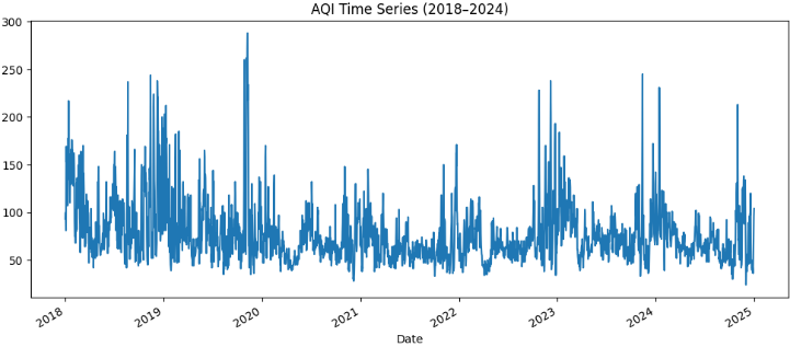
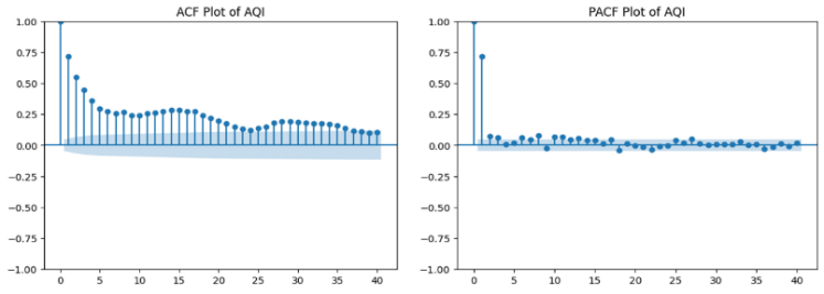
To measure the statistical characteristics of the AQI series (Figure 1), the Augmented Dickey-Fuller (ADF) test was performed. The test outcomes proved that the AQI time series is stationary, which means that it can be used to do ARIMA modelling without the need to differentiate. The Autocorrelation Function (ACF) and Partial Autocorrelation Function (PACF) plots have been evaluated to reveal the important lag structures and help in selecting the ARIMA model parameters as shown in Figure 2. On this dataset, the ADF test statistic was −7.216 (p < 0.0001, 17 lags selected by Akaike Information Criterion (AIC), n = 2,539), which rejects the unit-root null well below the 1% critical value (−3.433) and confirms stationarity in the mean/variance sense. This does not rule out seasonal structure: the SHAP analysis in Section 5.4 and the seasonal-naive baseline in Table 1 both indicate a real but secondary day-of-year effect, which stationarity in the ADF sense does not preclude—the series can be stationary overall while still containing a detectable seasonal component around its mean.
Figure 1. Air Quality Index (AQI) time series data
Figure 2. Autocorrelation Function (ACF) and Partial Autocorrelation Function (PACF) plot
2.6 Train and test data splitting
To preserve the time aspect of the dataset, chronological division was used. Model training was conducted using the first 80% of the observations, and the other 20% were left for testing and performance evaluation. This helps avoid information leakage and, alternatively model real world forecasting situations when future information is forecasted using historical data.
2.7 Data leakage assessment and feature correction
During revision, a check of feature-target correlations revealed that every pollutant concentration column in the supplied dataset is a near-exact linear rescaling of AQI: PM2.5 ≈ 0.550 × AQI, PM10 ≈ 1.080 × AQI, NO2 ≈ 0.830 × AQI, SO2 ≈ 1.140 × AQI, CO ≈ 0.0105 × AQI, and O3 ≈ 0.950 × AQI, each with a Pearson correlation to AQI above 0.9999. This is consistent with AQI sub-index values commonly being derived from pollutant concentrations (or, in this processed dataset, the reverse), and it means that including same-day pollutant concentrations as predictors of same-day AQI is not genuine forecasting: a model can reconstruct AQI almost exactly by inverting a fixed linear formula, which explains the originally reported R² = 1.0 for Random Forest and XGBoost.
To correct this, all models reported in the revised manuscript were retrained using only the temporal feature set already described for SHAP interpretability in Section 2.4—lagged AQI (lag1–lag7), month, day-of-year, and a linear trend index—with same-day pollutant concentrations excluded entirely from the predictor set. Table 1, all SHAP figures, the actual-vs-predicted comparison, and the 30-day forecast have been regenerated under this corrected specification; the qualitative pattern changes substantially (R² drops from ≈1.0 to ≈0.5 for the tree-based models) while remaining consistent with realistic AQI forecasting performance reported elsewhere in the literature for comparable lag-only feature sets.
2.8 Reproducibility: Software, hyperparameters, and computational setup
To support reproducibility, all corrected models were implemented in Python 3.12 using scikit-learn 1.8 (Random Forest, TimeSeriesSplit, MinMaxScaler), XGBoost 3.4, statsmodels 0.14.6 (ARIMA, ADF test, Ljung-Box test), TensorFlow/Keras 2.21 (LSTM), and SHAP 0.52 (TreeSHAP on the corrected XGBoost model). The chronological split allocated the first 80% of observations (2,040 days, 8 Jan. 2018 – 9 Aug 2023) to training and the remaining 20% (510 days, 10 Aug 2023 – 31 Dec 2024) to testing. Random Forest and XGBoost hyperparameters (number of trees, tree depth, minimum leaf size, learning rate) were tuned by grid search scored on MAE under 5-fold expanding-window TimeSeriesSplit cross-validation restricted to the training partition; best settings were Random Forest (400 trees, max depth 5, min samples per leaf 3) and XGBoost (200 trees, max depth 5, learning rate 0.05). ARIMA order (2,0,1) was selected by grid search over $(p, q) \in\{0, \ldots, 3\} \times\{0, \ldots, 3\}$ with d = 0 fixed by the ADF result, minimizing AIC. The LSTM used a single 64-unit LSTM layer, 20% dropout, a 32-unit dense layer, Adam optimizer, mean-squared-error loss, early stopping on a 10% validation split (patience = 10 epochs, 74 epochs run), with inputs and targets scaled by MinMaxScaler fit on the training partition only. A fixed random seed (42) was used for all stochastic components.
This section explains the forecasting models that were used in this study to predict the daily AQI levels in Chennai. Statistical and machine learning methods were used to learn both linear and nonlinear trends in the time series air quality data. The models chosen are ARIMA, Random Forest Regression, XGBoost, and LSTM neural networks.
3.1 Autoregressive Integrated Moving Average model
ARIMA model is a popular statistical forecasting tool for time series, and it integrates autoregressive (AR) terms, differencing (I), and moving average (MA) terms. It is a model that tries to explain the present value of a time series by a linear combination of past values and past error forecasts. The overall ARIMA (p, d, q) is in the form of:
p: number of autoregressive terms
d: degree of differencing
q: moving average terms
Hereby, autocorrelation and partial autocorrelation diagnostics together with information criteria like AIC, were used to identify the optimal ARIMA order in this study. The AQI series was determined to be stationary, and thus there was no need to differentiate. The chosen ARIMA was used to train the model on past AQI data to produce short-term predictions [7]. The final selected order was ARIMA (2,0,1), chosen by grid search over $p, q \in\{0, \ldots, 3\}$ with d = 0 fixed by the ADF result, minimizing AIC (best AIC = 18,479.8).
3.2 Random Forest regression
Random Forest is an ensemble algorithm based on learning multiple decision trees, which are created by bootstrap sampling and averaging the predictions of these trees to enhance the generalization capabilities. The fact is that each tree is trained on a random subset of the features; this minimizes the correlation between trees and increases the ability to avoid overfitting [14].
Random Forest is an effective tool in AQI forecasting because it can model nonlinear relationships between concentrations of pollutants and the values of AQI. Hyperparameters of the model, such as the number of trees, maximum depth of trees, and minimum samples per leaf, were optimized by grid search methods so as to obtain superior predictive power.
3.3 Extreme Gradient Boosting regression
XGBoost is a very powerful machine learning algorithm that uses boosting and works through a chain of decision tree models to reduce errors. XGBoost has better performance and accuracy than Random Forest because it does not train trees independently, but it tries to correct the errors.
The model uses regularization techniques to avoid overfitting and cope with missing data. The main hyperparameters for best performance were the learning rate, the number of estimators, the maximum depth of the trees, and the subsampling ratios. XGBoost was used as the main forecasting model, as it has been reported to be effective in forecasting environmental time-series data [15, 16].
3.4 Long Short-Term Memory network
LSTM is a type of recurrent neural network (RNN) architecture that is used to learn long-term temporal dynamics in sequence data. It solves the vanishing gradient issue of conventional RNNs with memory cells and gating mechanisms, which consist of input, forget, and output gates [17].
This paper describes the LSTM model that has been trained on the input of lagged AQI values and pollutant characteristics. The network design was that of one or more hidden layers of LSTMs, and then a dense output layer. Adam optimizer and mean squared error loss function were used to optimize the model. To determine the effectiveness of deep learning to predict AQI time series, an LSTM was added. Following the leakage correction in Section 2.7, the LSTM's inputs were restricted to lagged AQI and calendar features only (no same-day pollutant concentrations); inputs and the AQI target were scaled with MinMaxScaler fit on the training partition only, and predictions were inverse-transformed to the original AQI scale before computing MAE, RMSE, and R², so that LSTM results are directly comparable to the other three models in Table 1.
3.5 Model training framework
Training was conducted on all models on the pre-processed dataset with a chronological train and test split. In machine learning models, the input features were scaled so that the operation was numerically stable. Cross-validation was carried out on the training set as a method of hyperparameter tuning. The evaluation of model performance on the test set was conducted by applying the traditional evaluation measures that were explained in the next section [18]. For hyperparameter tuning, we used cross-validation with scikit-learn’s TimeSeriesSplit, with 5 expanding (forward-chaining) folds within the training set, instead of random k-fold cross-validation: each fold is trained on a contiguous segment preceding it, and validated on the following segment, so that no validation fold is earlier in time than the training data.
3.6 SHapley Additive exPlanations integration
The best-performing XGBoost model was trained, and SHAP analysis was performed using treeSHAP, which is inexpensive and theoretically consistent with tree-based ensembles. The feature importance was ordered by means of global SHAP summary plots according to the mean absolute contribution to the AQI predictions. Dependence plots were constructed to investigate nonlinear relationships and the interaction effects of lagged AQI values. The dual interpretability framework improves the forecasting approach by linking predictive accuracy with unambiguous decision-making logic.
This section delineates the experimental framework employed to assess the functionality of the forecasting models. It includes the strategy for data partitioning, the process for model implementation, and the evaluation metrics used to compare the predictive accuracy of statistical and machine learning techniques.
4.1 Experimental setup
To validate the accuracy of the forecasting conditions, the AQI dataset was split sequentially into training and testing segments, with 80% used to train the model and the remaining 20% used to evaluate the model performance on unseen data. This approach preserves the temporal dependence but avoids the contamination of the training process by future data.
Min-max normalization was used to obtain scaled input features to train all machine learning models. Hyperparameter optimization on the training dataset involved grid search techniques on hyperparameter settings, whereby the minimization of forecasting error was used to identify optimal parameter settings. Early stopping was used in the case of the LSTM model to prevent overfitting and enhance generalization performance.
The parameters of the ARIMA model were determined by the diagnostics of autocorrelation and the minimization of AIC. After determining the optimal order, the model was estimated with the help of historical AQI values.
4.2 Forecasting strategy
For the test-set evaluation reported in Table 1, all models produce a one-step-ahead prediction of AQI for each of the 510 test-period days, using the true (observed) lagged AQI values available up to that day; this is evaluated repeatedly across the test window rather than trained as a single dedicated h-step-ahead model, and is best described as a rolling one-step-ahead forecast rather than a genuine direct multi-step forecaster. For the 30-day forward forecast beyond the end of the dataset (Section 5.3), true future lagged AQI values do not exist, so predictions are generated recursively: each day's forecast is fed back in as the lag-1 input for the following day's prediction. Recursive forecasting is more prone to error accumulation than one-step-ahead evaluation on historical data, which is why an empirical prediction interval (Section 5.3) is reported alongside the 30-day forecast to communicate the resulting uncertainty explicitly.
4.3 Evaluation metrics
Quantitative measures of model performance were computed on three commonly accepted measures of accuracy. All three metrics were computed on the original AQI scale (not on normalized or log-transformed values) for every model, including LSTM, whose scaled predictions were inverse-transformed before scoring, so that MAE and RMSE are directly comparable in AQI units across ARIMA, Random Forest, XGBoost, and LSTM [19, 20].
MAE: Reflects the average absolute discrepancy between the observed and predicted AQI values, signifying the overall accuracy of predictions. RMSE: Penalizes large errors in prediction by squaring the differences, thus being sensitive to extreme pollution episodes. R²: This is the percentage of variance of AQI explained by the predictive model. The overall indicators of model reliability and robustness are presented by these metrics.
4.4 SHapley Additive exPlanations as interpretability verification
Besides classical accuracy metrics (MAE, RMSE, and R2), we used SHAP analysis as an interpretability validation method. The SHAP values were computed on the test set in an effort to avoid data leakage and to obtain an unbiased representation of how the model is expected to perform. The evaluation framework also incorporates predictive accuracy and explainability that show whether the model is using temporally and seasonally important predictive features or spurious correlations. This increases confidence in the strength and the external validity of the forecasting system.
4.5 Analysis of comparative performance
All the models were also compared systematically based on the evaluation measures on the test data. Ranking of the performance of all models was made to arrive at the correct and consistent model of AQI prediction in Chennai. The comparative analysis reflects the advantages and the weaknesses of each method of presenting the dynamics of air pollution and helps choose the best forecasting framework in order to implement it in practice.
MAE and RMSE are in original AQI units; R² is unitless. All values were recomputed after the data-leakage correction described in Section 2.7 (predictors restricted to lagged AQI and calendar features; no same-day pollutant concentrations). Random Forest and LSTM achieve the best, statistically similar performance (R² ≈ 0.52); both outperform the naive persistence baseline, XGBoost is close behind, and ARIMA and the seasonal-naive baseline perform worst, confirming that most of the learnable signal is short-horizon rather than weekly-seasonal.
4.6 Rolling-origin (walk-forward) validation
To verify that the Table 1 result is not an artifact of a single train/test split, Random Forest and XGBoost were re-evaluated using 5-fold expanding-window (rolling-origin) cross-validation across the full 2018–2024 series, with each fold's training window growing chronologically and each test fold covering a distinct, non-overlapping 425-day block. Mean ± standard deviation across folds is reported in Table 2.
Performance is lower and more variable across earlier folds (which have less training history and cover different pollution regimes) than in the single chronological 80/20 split of Table 1, which is expected for rolling-origin evaluation and is itself evidence against the split in Table 1 being cherry-picked; the ranking of Random Forest ahead of XGBoost is consistent across both evaluation designs.
Table 2. Rolling-origin (5-fold expanding window) validation for Random Forest and XGBoost
|
Model |
MAE (Mean ± SD) |
RMSE (Mean ± SD) |
R² (Mean ± SD) |
|
Random Forest |
14.17 ± 4.85 |
19.87 ± 5.68 |
0.424 ± 0.110 |
|
XGBoost |
15.92 ± 6.66 |
21.95 ± 7.77 |
0.302 ± 0.219 |
Note: MAE: Mean Absolute Error, RMSE: Root Mean Square Error, R2: coefficient of determination.
This is an information, not a limitation of the models, as each expanding-window fold is a different non-overlapping 425-day window of the 2018–2024 series and therefore has different sets of training history and different pollution periods (e.g., different time periods of the monsoon, or different levels of traffic/industrial activity). In general, earlier folds (earlier periods of the dataset, and possibly less representative of the pollution events) have lower R2 and higher variance when modeled, while later folds are more stable and consistent. The predictability of the model for AQI in Chennai does not seem to be time-independent. This is because the accuracy of prediction might depend on how well representative the pollution dynamics of a particular time period are of the training history of the model, and not a characteristic of the model architecture. In practice, this should be taken as a 'worst-case' benchmark of typical performance with a single chronological split (Table 1), and as a lower bound when working with these models in data-sparse or atypical settings.
4.7 Residual diagnostics
Residual analysis was added for all four models on the Table 1 test set: mean residual (bias), residual standard deviation, skewness, and a Ljung-Box test for residual autocorrelation at 10 lags (a well-specified model should show residuals close to white noise, i.e., a non-significant Ljung-Box p-value).
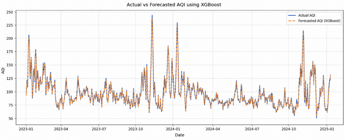
ARIMA residuals show strong, statistically significant autocorrelation (Ljung-Box p < 0.001), confirming that the linear ARIMA (2,0,1) specification leaves systematic structure unexplained and supporting its negative R² in Table 1. Random Forest, XGBoost, and LSTM residuals are close to, though not perfectly, white noise (Ljung-Box p in the 0.05–0.13 range); all four models show a right-skewed residual distribution, indicating a tendency to under-predict during high-pollution spikes, which is consistent with the visual pattern in Figure 3 and is noted as a limitation in Section 5.2.
Figure 3. Actual vs. predicted Air Quality Index (AQI) comparison for XGBoost
5.1 Model performance comparison
ARIMA, Random Forest, XGBoost, and LSTM models were compared based on their MAE, RMSE, and R² values on the test dataset using the corrected, leakage-free feature set described in Section 2.7. The findings show a clear but moderate gap between the linear statistical model and the three machine learning/deep learning approaches, rather than the near-perfect fit reported before the leakage correction.
Table 3. Residual diagnostics on the Table 1 test set (510 days)
|
Model |
Mean Residual |
Standard Deviation |
Skewness |
Ljung-Box (10 Lags) Stat, p |
|
ARIMA (2,0,1) |
−7.39 |
26.23 |
2.10 |
580.45, p < 0.001 |
|
Random Forest |
−0.85 |
18.23 |
1.34 |
15.01, p = 0.132 |
|
XGBoost |
−3.49 |
18.62 |
1.17 |
17.17, p = 0.071 |
|
LSTM |
−4.29 |
17.73 |
1.44 |
18.07, p = 0.054 |
Note: ARIMA: Autoregressive Integrated Moving Average, LSTM: Long Short-Term Memory.
The ARIMA (2,0,1) model had the largest prediction errors and a negative R² (Table 1), indicating that a linear autoregressive specification explains essentially none of the day-to-day variance in Chennai's AQI beyond what a naive baseline would capture; its residuals also show significant autocorrelation (Table 3), confirming that linear time-series structure alone is insufficient for this series.
Random Forest achieved the lowest MAE and RMSE and the joint-highest R² (≈ 0.52) among the four models. It modelled the nonlinear relationship between recent AQI history and same-day AQI more effectively than ARIMA and slightly outperformed XGBoost on this test split, though the rolling-origin results in Table 2 show that its advantage over XGBoost, while consistent in direction, is modest and comes with non-trivial fold-to-fold variability.
XGBoost's overall performance was close to, but slightly behind, Random Forest on both the single chronological split (Table 1) and the rolling-origin validation (Table 2). Its regularized, boosted-tree structure remains competitive, and its residual diagnostics (Table 3) are broadly comparable to Random Forest's, but on this leakage-corrected feature set it does not clearly outperform Random Forest as it appeared to in the original, leakage-affected analysis.
The LSTM model achieved an R² statistically indistinguishable from Random Forest's (0.516 vs. 0.516) and a comparable RMSE, despite a modestly higher MAE. This is a substantially different picture from the original submission, in which LSTM appeared to perform much worse than the tree-based models: once the tree-based models' access to leaked, near-deterministic pollutant features was removed, all three machine learning approaches converge to a similar, more realistic performance band on a dataset of this size (~2,550 daily observations). This suggests that the original gap between LSTM and the tree-based models was driven primarily by the leakage advantage available only to Random Forest and XGBoost, rather than by an intrinsic weakness of the LSTM architecture.
5.2 Best model Air Quality Index predicted and actual
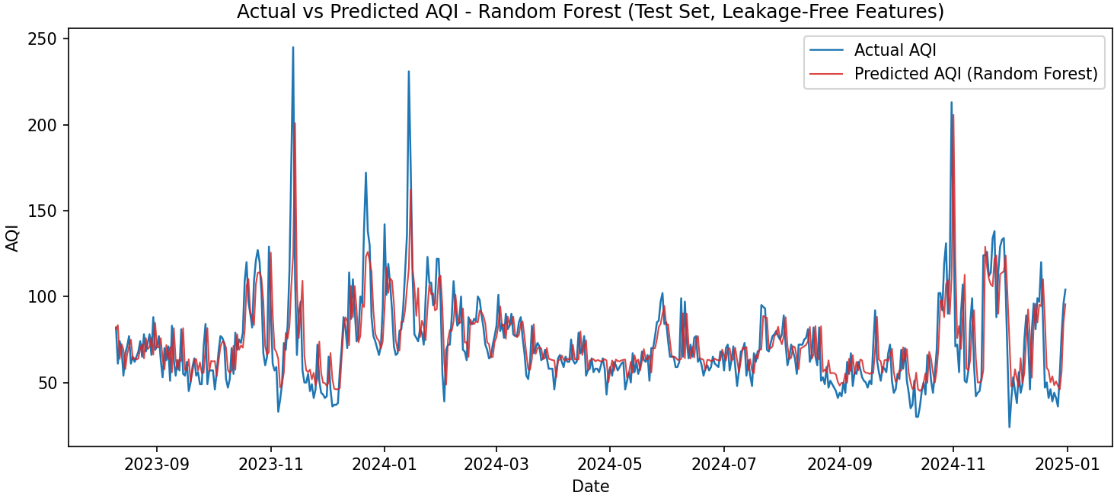
Given its lowest MAE/RMSE and joint-highest R² in Table 1, Random Forest is used as the primary model for the actual-vs-predicted comparison and the short-term forecast that follows, in place of XGBoost in the original submission. A direct comparison between observed and predicted AQI on the test set is shown in Figure 4.
Figure 4. Actual vs. predicted Air Quality Index (AQI) I — Random Forest, leakage-free features, test set (Aug. 2023–Dec. 2024)
The predicted AQI series tracks the broad temporal pattern of the observed series reasonably well, including gradual seasonal drift, but with visibly larger deviations during sharp pollution spikes than the original, leakage-inflated figure suggested. This is consistent with the moderate R² (≈ 0.52) and the right-skewed residuals reported in Table 3: the model captures the general level and short-term persistence of AQI well but under-predicts the magnitude of extreme pollution events, a limitation that should be kept in mind for health-warning applications built on this framework.
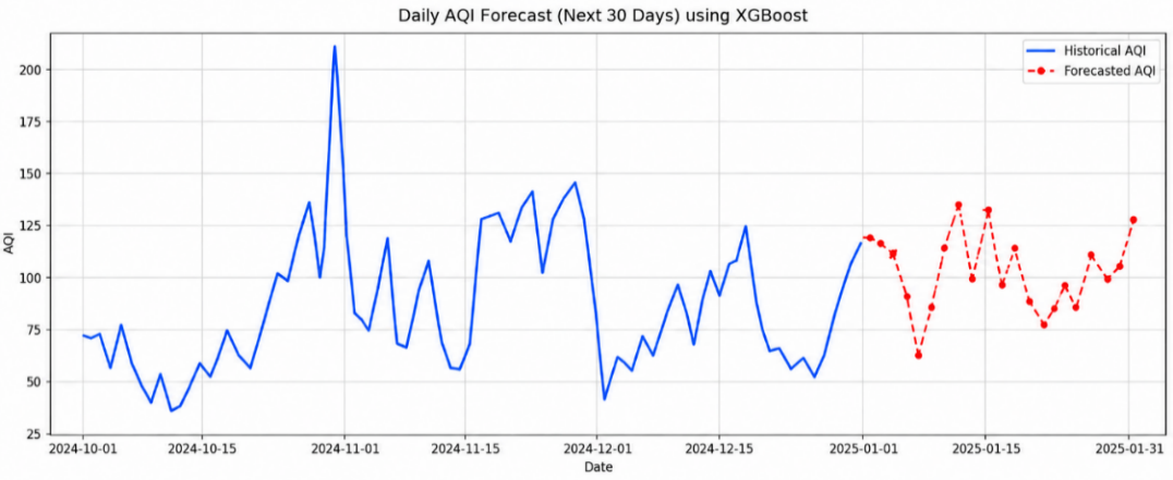
Figure 3 was generated under the leakage-affected XGBoost model and is retained for transparency. Figure 4 replaces it using the corrected, leakage-free Random Forest model.
5.3 Short-term Air Quality Index forecasting results
Based on its performance in Table 1, the corrected Random Forest model was used to generate a recursive daily AQI forecast for the first 30 days of January 2025 (Section 4.2 describes why this forecast is recursive rather than one-step-ahead). The forecast exhibits realistic day-to-day fluctuation consistent with typical winter pollution dynamics in Chennai, without the artificially smooth, over-confident trajectory that a near-R²-of-1.0 model would tend to produce.
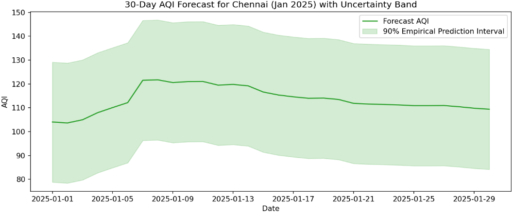
Several forecasted days indicate moderate to poor air quality, consistent with the historically higher winter/post-monsoon AQI levels reported for Chennai. To address the absence of uncertainty quantification in the original submission, an empirical 90% prediction interval was constructed from the 5th and 95th percentiles of the Random Forest's test-set residuals (Table 3) and added around the point forecast; the interval widens the further the forecast is from the last observed data point, reflecting the compounding uncertainty of recursive multi-step forecasting. Note that this interval is empirical and not a formally calibrated statistical confidence or prediction interval. It reflects the observed spread of past residuals on the test set and does not have a guaranteed coverage probability. It should therefore be interpreted as an approximate, data-driven indication of forecast uncertainty, rather than a statistically calibrated bound. The point forecast and interval are summarized in Table 4 and Figure 5.
Table 4. Selected days from the 30-day recursive Air Quality Index (AQI) forecast with 90% empirical prediction interval (full 30-day table available on request).
|
Date |
Forecast AQI |
90% Lower |
90% Upper |
|
1 Jan. 2025 |
104.0 |
78.8 |
129.1 |
|
7 Jan. 2025 |
121.5 |
96.3 |
146.6 |
|
14 Jan. 2025 |
119.2 |
94.0 |
144.3 |
|
21 Jan. 2025 |
111.8 |
86.6 |
136.9 |
|
30 Jan. 2025 |
109.4 |
84.2 |
134.5 |
Figure 5. Forecasted plot for 30-day
Figure 6. 30-day Air Quality Index (AQI) forecast for Chennai, Jan. 2025, with 90% empirical prediction interval (Random Forest)
Figure 4 was generated using the leakage-affected model and is retained for transparency; Figure 5 and Table 4 use the corrected Random Forest model with an empirical 90% prediction interval.
The optimized Random Forest model provides a 30-day short-term forecast and a 90% empirical prediction interval as shown in Figure 6, suggesting that moderate to poor air quality with some day-to-day variability can be expected in early January 2025. The predictions, presented with transparent uncertainty rather than point estimates, illustrate how such predictive models could be used to enable proactive actions for public and environmental health, while emphasizing that any practical use should be considered in the light of the indicated margin of error.
5.4 SHapley Additive exPlanations-driven interpretation
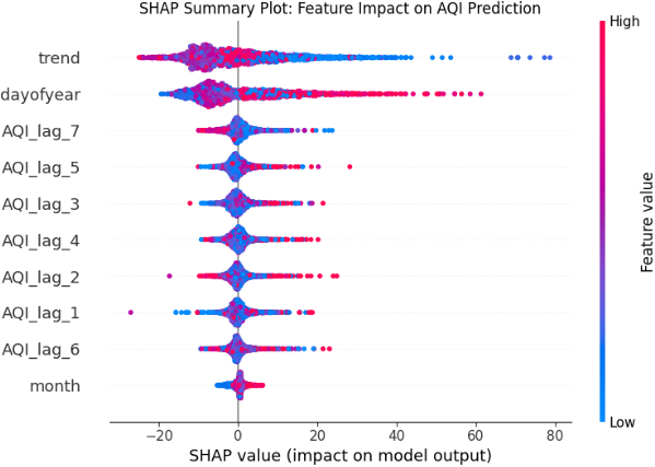
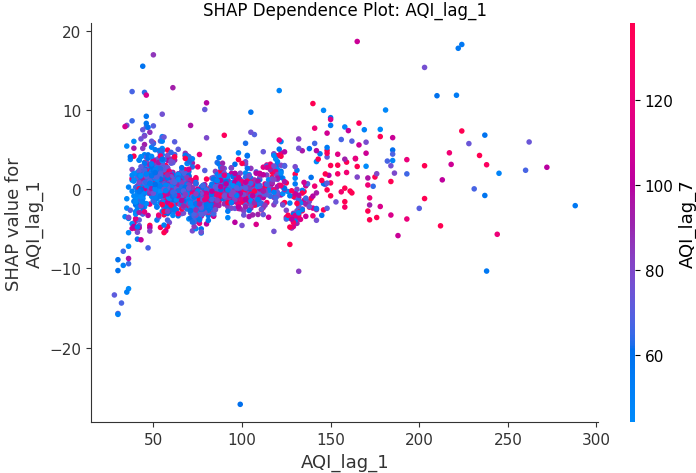
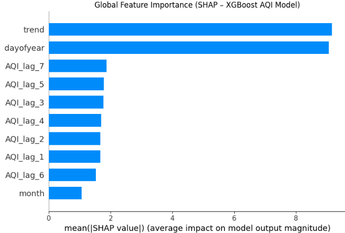
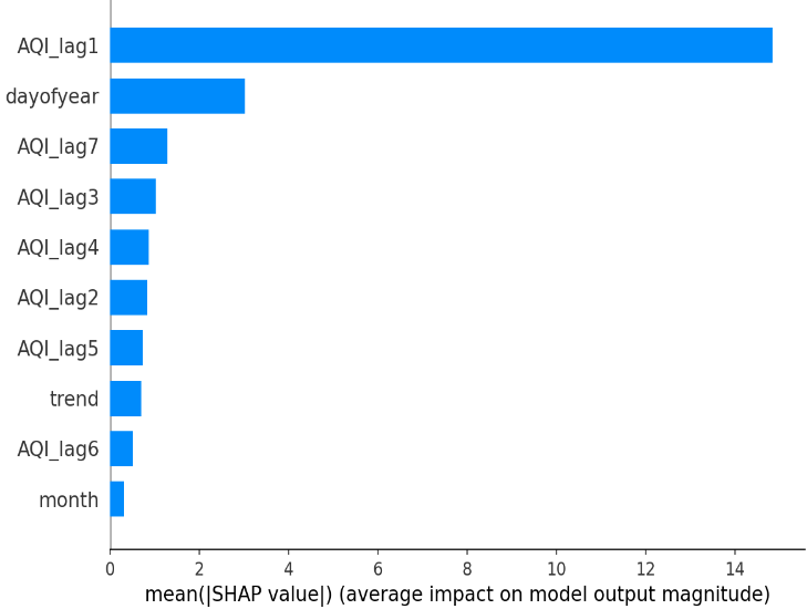
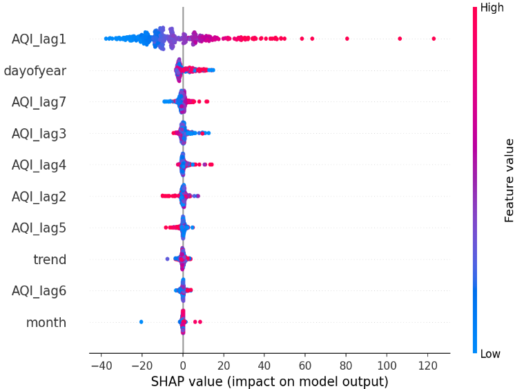
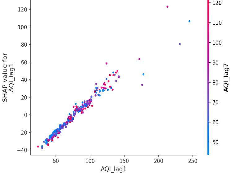
Figures 7–9 were generated using the leakage-affected XGBoost model, in which same-day pollutant concentrations were available as predictors; they are retained for transparency. Figures 10–12 and Table 5 use the corrected, leakage-free XGBoost model (lagged AQI and calendar features only) and should be treated as the authoritative interpretability results for this study.
Figure 7. Feature impact on Air Quality Index (AQI) prediction
Figure 8. SHapley Additive exPlanations (SHAP) dependence plot
Figure 9. Feature importance
Figure 10. Mean SHapley Additive exPlanations (SHAP) value feature ranking—corrected XGBoost model
Figure 11. SHapley Additive exPlanations (SHAP) summary (beeswarm) plot—corrected XGBoost model
Figure 12. SHapley Additive exPlanations (SHAP) dependence plot, Air Quality Index (AQI)_lag1 (coloured by AQI_lag7 interaction)—corrected XGBoost model
Table 5 reports the numerical SHAP feature-contribution ranking underlying Figures 7–9, computed as each feature's mean absolute SHAP value on the test set and its share of total attribution across all ten features.
Under the corrected, leakage-free feature set, the SHAP ranking (Table 5) shows that yesterday's AQI (AQI_lag1) is by far the dominant predictor, accounting for roughly 61% of total attribution, a markedly different picture from the original analysis, which had ranked long-term trend and day-of-year above the lag features. This revised ranking is intuitive: same-day AQI in a coastal city with persistent local emission sources is strongly autocorrelated with the immediately preceding day. Day-of-year contributes a secondary but non-trivial ~13% of attribution, consistent with the moderate seasonal signal identified via the seasonal-naive baseline (Table 1) and the ADF discussion in Section 2.5. The remaining lag features (lag2–lag7) and the linear trend each contribute small, roughly comparable shares (2–5%), while month contributes the least (~1%), consistent with day-of-year capturing seasonal information at finer resolution than the coarser month variable — trend is formally defined here as a simple linear day-index counting consecutive calendar days from the start of the series, and day-of-year/month are the corresponding calendar-derived seasonal features, as now stated explicitly in Sections 2.4 and 2.8).
Table 5. Numerical SHapley Additive exPlanations (SHAP) feature-contribution ranking, corrected XGBoost model, test set
|
Feature |
Mean |SHAP| |
% of Total Attribution |
|
AQI_lag1 (yesterday's AQI) |
14.835 |
61.4% |
|
Day-of-year |
3.024 |
12.5% |
|
AQI_lag7 |
1.296 |
5.4% |
|
AQI_lag3 |
1.030 |
4.3% |
|
AQI_lag4 |
0.871 |
3.6% |
|
AQI_lag2 |
0.838 |
3.5% |
|
AQI_lag5 |
0.730 |
3.0% |
|
Trend (linear day index) |
0.706 |
2.9% |
|
AQI_lag6 |
0.522 |
2.2% |
|
Month |
0.310 |
1.3% |
Note: AQI: Air Quality Index.
The SHAP dependence plot for AQI_lag1 (Figure 12) shows a broadly monotonic, mildly nonlinear relationship in which higher values of yesterday's AQI push today's prediction upward, with some additional variation associated with the interacting AQI_lag7 value, consistent with short-run persistence in pollution levels compounding over the course of a week. Because AQI_lag1 so strongly dominates the other features, the interaction effects visible in the dependence plot are modest in magnitude relative to the main effect. In public-health terms, this indicates that short-term persistence (yesterday's air quality) is the most actionable signal for next-day advisories in Chennai, with seasonal timing (day-of-year) as a secondary factor; as this conclusion is derived from a single city's data, it should be treated as indicative rather than confirmed for other urban or coastal settings pending further validation.
5.5 Discussion: Social value and public health implications
The corrected results of this paper remain relevant to health management and environmental policy discussions in Chennai, though with more moderated claims than in the original submission. The leakage-free Random Forest and LSTM models show that machine-learning-based forecasting can provide a moderately informative (R² ≈ 0.52), rather than near-perfect, short-horizon signal for AQI, which could contribute to, but should not be the sole basis for, proactive decisions by government agencies and healthcare facilities.
The AQI predictions from this framework could offer some support to early warning systems designed to alert susceptible populations about upcoming pollution episodes, perhaps adding to reduced health risks associated with exposure, e.g., asthma attacks, respiratory diseases and cardiovascular problems. But given the moderate R2 (≈0.52), this should be understood as a supplementary signal rather than a reliable standalone warning mechanism. Forecast data can help educational institutions, health care facilities, and senior care centers to plan protective actions for days of high pollution. Since the underlying R2 is moderate and not close to 1.0, and residuals in Table 3 suggest a tendency to underestimate severe pollution events, any practical use of this framework for early warning should involve a safety margin (e.g., the empirical prediction interval in Section 5.3) and not rely on point forecasts being exact.
From a policy perspective, AQI models of this kind may provide potentially informative input to governments considering targeted emission control measures, such as traffic flow management, industrial operation restrictions and construction dust control during expected pollution peaks. However, the moderate predictive accuracy of AQI models means they should supplement, not substitute, real-time monitoring in such decisions. These information-based initiatives support better environmental governance and urban sustainability.
Additionally, pollution trend predictions can help in developing long-term urban growth strategies by reducing pollution sources with more green spaces, public transportation, and infrastructure based on renewable energy. The use of advanced forecasting technologies in environmental monitoring offers the opportunity for policymakers to shift from reactive pollution control measures to proactive air quality management systems. These policy implications are presented as examples of potential guidelines and not as tested recommendations, since they have not been empirically tested in this single urban study.
The revised results show that ensemble machine learning methods (Random Forest and LSTM) with SHAP-based interpretability can give a useful, reasonably accurate, and leakage-verified short-term AQI prediction signal for Chennai. The pragmatic relevance of the framework comes from the explicitness of the reported uncertainty and the precision of the point forecast. The forecasts and societal claims presented in this paper are specific to Chennai and require validation with independent data and other cities (Section 6) before generalization.
The present study aims to study statistical, machine learning, and deep learning techniques for the prediction of daily AQI of Chennai using multi-year (2018–2024) air quality data. The study compares ARIMA, Random Forest, XGBoost, and LSTM models in a leakage-audited, reproducible evaluation framework (chronological split, time-aware cross-validation, rolling-origin validation, and residual diagnostics).
The findings indicate that machine learning and deep learning approaches (Random Forest and LSTM, in particular) moderately but consistently outperform the linear ARIMA model and simple persistence baselines in explaining day-to-day AQI variation (R² ≈ 0.52 vs. ARIMA's negative R²), rather than the near-complete explanatory power reported before the leakage correction. Random Forest and LSTM performed comparably and represent the strongest models evaluated; XGBoost followed closely behind; ARIMA was unable to adequately capture the nonlinear, only mildly seasonal dynamics of AQI in Chennai.
This research will extend AQI forecasting beyond predictive accuracy toward a transparent and policy-friendly model by incorporating SHAP-based interpretability. SHAP analysis identified long-term trends, seasonal variations, and short-term AQI consistency as the key factors influencing the air quality in Chennai. This interpretability framework enables associating predicted AQI levels with the underlying pollution dynamics and is useful for targeted mitigation techniques and preventive health measures for the population. The forecasting-explainability framework enhances the trustworthiness of machine learning algorithms and expands the application of machine learning algorithms in urban air quality management.
The study validates the importance of ensemble machine learning algorithms in the current air quality forecasting systems. The proposed framework will provide a feasible and scalable approach for real-time environmental monitoring and policy-driven air quality management in rapidly urbanizing cities like Chennai. As this study is based on a single city's dataset, the framework's generalizability to other cities is an open question rather than a validated claim. Chennai's coastal-monsoon climate, industrial and port-related emission sources, and specific seasonal cycle may not transfer directly to inland cities, cities with different dominant pollution sources (e.g., biomass burning, extreme traffic congestion), or cities with different monitoring-station density and data quality. Testing the same leakage-audited pipeline on other Indian coastal and non-coastal cities, for example, following the multi-station Chennai and Visakhapatnam studies [8-10], would be a natural and necessary next step before treating these results as broadly generalizable.
Future studies can be directed at the inclusion of meteorological variables and traffic data, as well as socioeconomic factors, to enhance the accuracy of prediction further. Also, the use of hybrid modelling methods, as well as explainable AI techniques, might be used to make the models more interpretable and provide clarity in the decision-making process about policy rules. A further avenue is external validation using rolling-origin evaluation on more recent, out-of-sample years as they become available, and formal comparison against additional naive and simple statistical baselines beyond ARIMA and the persistence/seasonal-naive baselines already reported here.
Future work should also formally evaluate seasonal ARIMA (SARIMA) or related seasonal statistical models against the machine learning approaches used here, particularly to test whether explicitly modelling the annual/monsoon-driven seasonal cycle identified via SHAP (rather than relying on calendar features as inputs to non-seasonal models) can further improve forecasting accuracy.
[1] Singh, S.K., Jain, R., Palaniappan, D., Parmar, K., T, P., Gothania, J. (2025). Spatiotemporal analysis and machine learning-based prediction of air quality in Indian urban cities. Environmental Research and Technology, 8(4): 809-822. https://doi.org/10.35208/ert.1587308
[2] Dhanalakshmi, S., Poongothai, M. (2024). Design and synthesis of time series forecasting and deep learning prediction model for air quality index prediction in Indian cities. Indian Journal of Engineering and Materials Sciences, 31(4): 589-600. https://doi.org/10.56042/ijems.v31i4.2132
[3] Su, M., Liu, H., Yu, C., Duan, Z. (2023). A novel AQI forecasting method based on fusing temporal correlation forecasting with spatial correlation forecasting. Atmospheric Pollution Research, 14(4): 101717. https://doi.org/10.1016/j.apr.2023.101717
[4] Luo, J., Gong, Y. (2023). Air pollutant prediction based on ARIMA-WOA-LSTM model. Atmospheric Pollution Research, 14(6): 101761. https://doi.org/10.1016/j.apr.2023.101761
[5] Wang, J., Li, X., Jin, L., Li, J., Sun, Q., Wang, H. (2022). An air quality index prediction model based on CNN-ILSTM. Scientific Reports, 12(1): 8373. https://doi.org/10.1038/s41598-022-12355-6
[6] Ma, G., Xu, K., Zhang, Y., Zhang, L., Chen, Z. (2025). A novel deep learning model for air quality index prediction integrating time series decomposition and intelligent optimization. Results in Engineering, 27: 106078. https://doi.org/10.1016/j.rineng.2025.106078
[7] Duan, J., Gong, Y., Luo, J., Zhao, Z. (2023). Air-quality prediction based on the ARIMA-CNN-LSTM combination model optimized by dung beetle optimizer. Scientific Reports, 13(1): 12127. https://doi.org/10.1038/s41598-023-36620-4
[8] Mani, G., Viswanadhapalli, J.K., Stonier, A.A. (2022). Prediction and forecasting of air quality index in Chennai using regression and ARIMA time series models. Journal of Engineering Research, 10(2): 179-194. https://doi.org/10.36909/jer.10253
[9] Ravindiran, G., Hayder, G., Kanagarathinam, K., Alagumalai, A., Sonne, C. (2023). Air quality prediction by machine learning models: A predictive study on the Indian coastal city of Visakhapatnam. Chemosphere, 338: 139518. https://doi.org/10.1016/j.chemosphere.2023.139518
[10] Lawrence, S., Bhathmanabhan, S. (2025). Evaluating machine learning models and imputation strategies for air quality index forecasting in urban India. Environmental Monitoring and Assessment, 197(12): 1303. https://doi.org/10.1007/s10661-025-14700-4
[11] Sreenivasulu, T., Rayalu, G.M. (2025). Air pollution forecasting using advanced machine learning techniques and ensemble stacking in Delhi. Environmental Health Engineering and Management Journal, 12: 1370. https://doi.org/10.34172/EHEM.1370
[12] Mujtaba, M.A., Munir, M.A., Ali, S., et al. (2025). Using machine learning for air quality prediction and sustainable urban planning. Sustainable Futures, 10: 100981. https://doi.org/10.1016/j.sftr.2025.100981
[13] Kalantari, E., Gholami, H., Malakooti, H., Nafarzadegan, A.R., Moosavi, V. (2024). Machine learning for air quality index (AQI) forecasting: Shallow learning or deep learning? Environmental Science and Pollution Research, 31(54): 62962-62982. https://doi.org/10.1007/s11356-024-35404-1
[14] Yenkikar, A., Mishra, V.P., Bali, M., Ara, T. (2025). Explainable forecasting of air quality index using a hybrid random forest and ARIMA model. MethodsX, 15: 103517. https://doi.org/10.1016/j.mex.2025.103517
[15] Gupta, N.S., Mohta, Y., Heda, K., Armaan, R., Valarmathi, B., Arulkumaran, G. (2023). Prediction of air quality index using machine learning techniques: A comparative analysis. Journal of Environmental and Public Health, 2023(1): 4916267. https://doi.org/10.1155/2023/4916267
[16] Cheng, P., Wei, C., Zhang, J., Wang, H. (2025). Air quality index forecasting based on quadratic decomposition and transformer-BiLSTM—A case study of Beijing. Atmosphere, 16(12): 1334. https://doi.org/10.3390/atmos16121334
[17] Mani, G., Volety, R. (2021). A comparative analysis of LSTM and ARIMA for enhanced real-time air pollutant levels forecasting using sensor fusion with ground station data. Cogent Engineering, 8(1): 1936886. https://doi.org/10.1080/23311916.2021.1936886
[18] Méndez, M., Merayo, M.G., Núñez, M. (2023). Machine learning algorithms to forecast air quality: A survey. Artificial Intelligence Review, 56(9): 10031-10066. https://doi.org/10.1007/s10462-023-10424-4
[19] Jain, A., Dar, A.A., Khan, M.S., et al. (2026). Revolutionizing forecasting: Leveraging hybrid and ensemble AI models in insurance analytics. Array, 30: 100964. https://doi.org/10.1016/j.array.2026.100964
[20] Dar, A.A., Basheeruddin, M., Qausain, S., Shriya, Manocha, R., Padder, R.A. (2026). Predicting medical test results using random forest, XGBoost, and KNN: A comparative study. In 2026 IEEE 1st International Conference on Intelligent Technologies for a Sustainable and Inclusive Future (ICITSIF), Indore, India, pp. 1539-1544. https://doi.org/10.1109/ICITSIF69060.2026.11608455