Sudha Rani Kandru*![]() | Sumalatha Akunuri
| Sumalatha Akunuri![]() | Kusuma Tummala
| Kusuma Tummala![]() | Manjula Sri Rayudu
| Manjula Sri Rayudu![]() | J. Bhavani
| J. Bhavani![]()
© 2026 The authors. This article is published by IIETA and is licensed under the CC BY 4.0 license (http://creativecommons.org/licenses/by/4.0/).
OPEN ACCESS
Accurate discrimination between edible and poisonous mushrooms is important for food safety, particularly when identification relies on external morphological traits that may be difficult to interpret visually. This study presents a comparative machine learning framework for predicting mushroom edibility using a public Mushroom Classification dataset containing 8,124 samples and 22 categorical morphological attributes, including cap shape, cap color, odor, gill characteristics, stalk features, and habitat. After label encoding and feature preprocessing, the dataset was divided into training and testing subsets using an 80:20 split. Six classification models were implemented and compared: Bayesian Ridge, Huber Regressor, Elastic Net with Nearest Centroid, Kernel Ridge with RBF Sampler, Nearest Centroid Classifier with Lasso, and Passive Aggressive Classifier with Isolation Forest. Model performance was assessed using accuracy, precision, recall, F1-score, Matthews correlation coefficient (MCC), area under the receiver operating characteristic curve, Cohen’s kappa coefficient, and confusion matrix analysis. Among the evaluated models, the Nearest Centroid Classifier with Lasso achieved the best overall performance, with an accuracy of 98.03%, precision of 97.97%, AUC of 0.9803, and Cohen’s kappa of 96.06%. The results indicate that sparse feature selection combined with centroid-based classification can provide reliable discrimination between edible and poisonous mushrooms in categorical tabular datasets. This work also shows that odor- and gill-related attributes are particularly informative for mushroom edibility prediction.
mushroom edibility prediction, poisonous mushroom classification, machine learning, morphological traits, feature selection, nearest centroid classifier, Lasso regularization
Mushrooms are a diverse collection of fungus which have been used for food for ages and have a long history in many different cuisines around the world. But this wide group also contains species that, if consumed, may be fatally poisonous. It is critical to be able to differentiate between toxic and edible mushrooms in order to protect consumers, cooks, and foragers. Mushrooms are members of the Fungi, a distinct class of organisms. They thrive on decomposing organic debris and lack the green substance (chlorophyll) found in plants. Through the use of extremely tiny, thread-like structures called mycelium, which pierce the substratum and tend to be invisible on the surface, they are able to take nutrients from these decomposing substrates. Building of essential infrastructure is necessary for the seasonally cultivated white button mushroom in India, which is grown in climate-controlled crop houses.
Regression, Huber Regressor, Elastic Net with Nearest Centroid, Kernel Ridge with Radial Basis Function (RBF) Sampler. Nearest Centroid Classifier with Lasso, Passive Aggressive Classifier Isolation Forest.
Because certain mushrooms are extremely toxic, classifying them is essential to maintaining food safety and averting health hazards. With the use of numerous features, this research aims to precisely categorize mushrooms as edible or deadly by creating and comparing a number of machine learning (ML) and deep learning (DL) models. Information about mushroom properties, including color, shape, smell, and more are included in the dataset that was used for this project. Evaluation of various models' predictive power for mushroom edibleness and analysis of their advantages and disadvantages are the main goals. Among the many models selected are classic ML algorithms like Bayesian Ridge Regression, Huber Regressor, Elastic Net with Nearest Centroid, Kernel Ridge with RBF Sampler. Nearest Centroid Classifier with Lasso, Passive Aggressive Classifier Isolation Forest.
Ria et al. [1] discussed the differences between the recognition of Poisonous and non poisonous. The drawback for this paper is that the authors used only five commonly used algorithms for comparison with only accuracies. Sutayco et al. [2] identified medicinal mushrooms using computer vision techniques and convolutional neural networks (CNN). The focus is on leveraging advanced technologies for automated recognition and classification of medicinal mushroom species. The drawback for this paper is the authors used only two algorithms for comparison with only accuracies. Zahan et al. [3] explained the different categories of mushrooms. DL methods likely involve neural networks for improved accuracy and complexity in distinguishing between different mushroom types. Saryoko et al. [4] likely involved the utilization of predictive modeling techniques to forecast mushroom yields or characteristics based on specific features. The drawback for this paper is the authors used only six commonly used algorithms for comparison with only accuracies. Long et al. [5] explained wild mushroom classification. This involves developing a ML model, specifically an improved version of MobileViT_v2, to accurately categorize wild mushrooms based on certain characteristics. The drawback for this paper is the authors used only few commonly used algorithms for comparison with only accuracies.
Dong et al. [6] primary objective of the paper is to address the quality classification of Enoki mushroom caps. The focus is on developing a classification system using CNN to assess and categorize the quality of Enoki mushroom caps. The drawback for this paper is the authors used only one commonly used algorithm. Verma and Dutta [7] explored and compare the use of two different computational methods, Artificial Neural Networks for the classification of mushrooms. The drawback for this paper is the authors used only two commonly used algorithms for comparison. Wibowo et al. [8] discussed a classification algorithm specifically designed for the identification of edible mushrooms. The drawback for this paper is the authors used only three commonly used algorithms for comparison with only accuracies. Ottom et al. [9] discussed the classification of mushroom fungi. Kanchi et al. [10] explained the mushroom classification. The drawback for this is the authors used only six commonly used algorithms for comparison with only accuracies and Receiver Working Characteristic (ROC) curves.
YOLOv5 was utilised by Moysiadis et al. [11] to recognize the phases of mushroom development and specify which ones were ready for harvest. According to the results, it can identify mushrooms in the greenhouse with a 76% detection rate. The final stage of mushroom growth allows for up to 70% accuracy in classification. Ismail et al. [12] had calculated mushroom behavioral structures to novelty out the finest feature for categorizing dissimilar categories of mushrooms. Ketwongsa et al. [13] presented a new DL model established on an improved AlexNet CNN. While cutting down on training and testing time, this model showed excellent accuracy in differentiating between edible and toxic mushrooms. Using a smartphone app driven by a CNN, Lee et al. [14] created a technique to categorise different kinds of mushrooms from field-collection photos. This method demonstrates how ML can be used to classify mushrooms. The goal of Chong et al. [15] was to make an Internet of Things (IoT)-based conservational one-to-one care and control system for mushroom cultivation. Pal et al. [16] examined behavioural attributes of mushrooms such as the structure, size of the surface, cap tone, lamella, which is also known as the gill, and stalk as well as the smell place where the mushroom was grown, and population. The ML algorithm we will use would be K Means clustering. Moysiadis et al. [17] suggested a system architecture based on cutting-edge technologies and data collection for a mushroom greenhouse. In addition, the greenhouse's atmospheric conditions and the substrate's characteristics are crucial for growing mushrooms. According to Eben et al. [18], the goal of the study is to automate the mushroom production plant and monitor the environmental conditions in the crop room in order to minimise the amount of human care needed for the mushroom plant. An Android app-based solution to the issue was suggested by Jacob et al. [19]. Using the machine vision concept, the app will scan the mushroom image and determine whether it is edible or not. Training and classification are accomplished through the use of CNN classification algorithms. To make mushroom cultivation simpler and more effective, they also created an automated mushroom house. Chumuang et al. [20] used the physical data of twenty-two attributes from eight hundred samples to develop a ML model for classifying mushrooms. It was separated into two categories: non-toxic and toxic.
Previous works achieved reasonable classification accuracy, but many works were based on limited datasets, few classification algorithms, or only accuracy metrics without robustness measures such as Matthews correlation coefficient (MCC), Area Under Curve (AUC), and Cohen’s Kappa Coefficient (CKC). Moreover, many studies only focused on CNN-based image classification and did not evaluate ML approaches, based on tabular features. To overcome these limitations, the present work performs an extensive comparative analysis of various ML and DL models using a wide range of evaluation metrics for accurate mushroom edibility prediction.
Edible and toxic mushrooms were categorised using the Mushroom Classification dataset, which includes morphological characteristics like cap shape, colour, and odour. Before the model was trained, all categorical variables were standardised and numerically encoded. Several machine learning models were used, such as Huber Regressor, Bayesian Ridge, Elastic Net with Nearest Centroid, Kernel Ridge with RBF Sampler, Nearest Centroid with Lasso, and Passive Aggressive Classifier with Isolation Forest. Confusion matrix analysis and accuracy metrics were used to train and assess each model. To identify the best classification strategy, a comparative performance evaluation was carried out.
3.1 Methodology
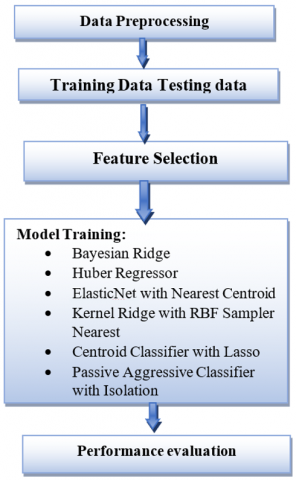
The Process Flow for the mushroom classification as shown in Figure 1 research involves several key steps, from Data Loading to Data Visualization. The different stages consist of Mushroom dataset, Data preprocessing, Label encoding, Data training, Data Testing, Classification Algorithm, Classifier model, Prediction, Evaluation, Accuracy, Classification Report, Model Comparison using data visualization tools.
In this study, the Mushroom Classification dataset is used which contains morphological characteristics of mushrooms such as cap shape, cap color, odor, gill size, stalk shape, and habitat information. The dataset contains 8124 samples with 22 categorical attributes for classification into two classes: edible (C₀) and poisonous (C₁). The dataset contains categorical features and during preprocessing label encoding techniques were used. The dataset did not contain any missing values and thus there was no need for data imputation methods. The dataset for model evaluation was divided into 80% for training data and 20% for testing data Feature importance methods were employed to examine the important features such as odor, gill color, cap color and stalk characteristics. The analysis showed that the features related to odor and gill play an important role in prediction of edible and poisonous mushrooms.
Figure 1. Block diagram of mushroom classification algorithm
The choice of the models was based on their capability to deal with mushroom features as categorical, feature sparsity, non-linearity and robustness to noisy or outlier data. We chose Bayesian Ridge and Huber Regressor for regularization and outliers, and Kernel Ridge with RBF Sampler for non-linear relationships. Nearest Centroid with Lasso was used to guarantee feature selection and classification performance stability. In the revised manuscript, we have added a detailed explanation and a model selection table in the Methodology section.
Firstly, mushroom classification dataset containing information about the characteristics of different mushrooms and their edibility. This is followed by data exploration and understanding, including performing. The data is then preprocessed using appropriate techniques, including handling any missing values using label encoding or one-hot encoding. Features (X) and target variable (y) have been divided from the dataset. Model selection then follows, choosing between different models for classification, including traditional ML models and DL architectures. The selected models are Bayesian Ridge Regression, Huber Regressor, Elastic Net with Nearest Centroid, Kernel Ridge with RBF Sampler, Nearest Centroid Classifier with Lasso, Passive-Aggressive with Isolation Forest.
For regularization, Bayesian principles have been used. Estimate the uncertainty associated with model parameters. Compared to traditional least squares regression, the Huber regression model is a robust regression model that is less prone to outliers. Elastic Net with Nearest Centroid: Combine Elastic Net regression and Nearest Centroid classification for feature selection. Use both L1 and L2 normalization for feature weighting. Kernel Ridge with RBF Sampler is Kernel Ridge Regression combines ridge regression and kernel tricks. The Nearest Centroid classifier with Lasso uses Nearest Centroid classification after feature selection with Lasso regression. Lasso helps select sparse features and improves interpretability. Passive Aggressive Classifier Classifier with Isolation Forest uses the Passive Aggressive Classifier Classifier with Isolation Forest classifier for anomaly detection.
The hyperparameters of the implemented machine learning models were chosen based on experimental evaluation and standard optimization settings to achieve stable predictive performance. In the Lasso model, the alpha value was set to 0.01 to control the regularization of features and sparsity of the model. The epsilon parameter of the Huber Regressor was set to be 1.35 for more robustness to outliers. A Kernel Ridge model was used with gamma = 0.1 to control the kernel and model complexity. These parameter settings were selected from many experimental observations, to get the best classification accuracy and generalization performance.
To evaluate model generalization, data splitting involves dividing the preprocessed information into sets for training and testing. Model-Specific Preprocessing is to apply model-specific preprocessing steps, such as standardization, tokenization, or embedding, based on the requirements of each selected model. The purpose of model training is for appropriate training algorithm for train every model upon the training set. Model assessment is Analyze the performance of the trained models using the testing set. Use accuracy as the primary metric for classification models. Generate classification reports to analyze precision, recall, and F1-score for each class. Results Analysis is to analyze and interpret the results, identifying models that demonstrate high accuracy and reliable classification performance. Model Comparison: such as Model Accuracy Comparison Bar Plot and Table, Precision Comparison Line Chart, MCCs Comparison Line Chart, Model AUC Distribution Pie Chart, Cohens Kappa Coefficients Comparison Line Chart and ROC Curves Comparison. The various statistical metrics that are evaluated are as shown below.
If the Positive class is predicted correctly, then the class is called True Positives $\tau_P$ (Class 1).
If negative instances are predicted correctly, then the class is called True Negative $\tau_N$.
If positive instances are incorrectly predicted, then it is called False Positive $F_P$ (class 0 predicted as class 1).
If negative instances are predicted incorrectly then it is called False Negative $F_N$ (class 1 predicted as class 0).
Accuracy is the proportion of correctly classified instances, which is calculated as
Accuracy $=\tau_P+\tau_N / \tau_P+\tau_N+F_P+F_N$ (1)
Precision is the proportion of true positive predictions among all positive predictions, calculated as
Precision $=\tau_P /\left(\tau_P+F_P\right)$ (2)
Recall (Sensitivity) is the proportion of true positive predictions among all actual positives, calculated as
Recall $=\frac{\tau_P}{\tau_P+F_N}$ (3)
F1 Score is the harmonic mean (HM) of precision and recall, provided that a stability between the dual metrics, planned as
$F 1=2 \times \frac{\text {Precision} \text { × } \text {Recall}}{\text {Precision}+ \text {Recall}}$ (4)
For Class 0 $C_0$:
Precision ($C_0$) is the precision precisely for $C_0$, find as
Precision $_{C_0}=\tau_N /\left(\tau_N+F_N\right)$ (5)
Recall ($C_0$) is the recall specifically for $C_0$, find as
$\operatorname{Recall}_{C_0}=\frac{\tau_N}{\tau_N+F_p}$ (6)
F1 Score ($C_0$) is the F1 score definitely for $C_0$, calculated as
$F 1$ Score $_{C_0}=\frac{2 \times\left(\text {Precision}_{C_0} \times \text {Recall}_{C_0}\right)}{\left(\text {Precision}_{C_0}+\text {Recall}_{C_0}\right)}$ (7)
For Class 1 $C_1$:
Precision ($C_1$) is the precision specifically for $C_1$, calculated as
Precision $_{C_1}=\frac{\tau_P}{\tau_P+F_p}$ (8)
Recall ($C_1$) is the recall specifically for $C_1$, calculated as
Recall $_{C_1}=\frac{\tau_P}{\tau_P+F_N}$ (9)
F1 Score ($C_1$) is the F1 score specifically for $C_1$, calculated as
$F 1$ Score $_{C_1}=\frac{2 \times\left(\text {Precision}_{C_1} \times \text {Recall}_{C_1}\right)}{\left(\text {Precision}_{C_1}+\text {Recall}_{C_1}\right)}$ (10)
MCC is a correlation coefficient among the experimental and projected binary organizations, ranging from -1 to +1. A coefficient of +1 signifies a textbook estimate, 0 symbolizes no better than random prediction, and -1 represents total disagreement between prediction and observation.
$\begin{aligned} & M C= \frac{\left(\tau_P \times \tau_N-F_p \times F_N\right)}{\sqrt{\left(\tau_P+F_p\right) \times\left(\tau_P+F_N\right) \times\left(\tau_N+F_p\right) \times\left(\tau_N+F_N\right)}}\end{aligned}$ (11)
Area under the ROC curve (AUC) is the part under the ROC curve, which events the aptitude of the model to differentiate between positive and negative classes. AUC ranges from 0 to 1, with higher values indicating better performance.
$A U C=(1 / 2)-(F P R / 2)+(T P R / 2)$ (12)
where, the False Positive Rate (FPR) measures the proportion of actual negative cases that are incorrectly classified as positive by the classifier.
CKC is a measurement that processes inter-rater arrangement for categorical items. It considers how much better the arrangement is over what would be credible by chance, with values closer to 1 indicating better agreement.
Cohen's Kappa Coefficient
$\kappa=\frac{2\left[\left(\tau_P \times \tau_N\right)-\left(F_N \times F_P\right)\right]}{\left(\tau_P+F_P\right)\left(F_P+\tau_N\right)+\left(\tau_P+F_N\right)\left(F_N+\tau_N\right)}$ (13)
The data set was divided into 80% training and 20% testing data with random state 42 for reproducibility. Label encoding and feature normalization techniques were applied in pre-processing. The models were built in Python using the Scikit-learn and TensorFlow libraries. Hyperparameters were experimentally optimized for each model. Performance evaluation was carried out using Accuracy, Precision, Recall, F1-score, MCC, AUC and Cohen’s Kappa metrics.
In order to accurately identify between edible and hazardous mushrooms, in this study on the classification of mushrooms, we looked into a variety of ML and DL models. The wide variety of models demonstrated their distinct qualities and offered insightful information on how well they performed for this particular task.
4.1 Bayesian Ridge
Confusion Matrix for Bayesian Ridge has shown in the Figure 2(a). Out of 2438 mushroom test data , true positives are 1207 which indicates that the model correctly predicted 1207 instances of $C_1$ as $C_1$, true negatives are 1090, import the model correctly predicted 1090 cases of class 0 as class 0, false positives are 87, meaning the model incorrectly predicted 87 occurrences of $C_0$ as $C_1$, and false negatives are 54, implication the model inaccurately predicted 54 occurrences of $C_1$ as $C_0$.
Performance Metrics of Bayesian Ridge has shown in the Figure 2(b). The Overall accuracy of the model is 94.22%, which means the model makes accurate predictions 94.22% of the all the times. When Precision has been considered, the precision is 93% for class 0 and the precision is 95% for class 1. This suggests that, for class 0 and class 1, the model predicts as poisonous mushrooms correctly around 93% of all the times and 95% edible mushrooms of all the times, respectively. When Recall has been considered, the recall is 96% for class 0 and the recall is 93% for class 1. This indicates that 96% of the real class 0 occurrences and 93% of the real class 1 instances can be captured by the model. When F1-score has been considered, the F1-score for both classes is 94%, which shows that recall and precision are well-balanced. When Support has been considered, the 1261 instances are there for class 0 and 1177 instances are there for class 1. The Precision of the model is 95.28%. The MCC of the model is 0.8844. The AUC of the classic is 94.16%. The CKC of the model is 88.41%.
Parameters-TP, TN, FP, FN for Bayesian Ridge has shown in the Figure 2(c), Out of 100 percent mushroom test data , true positives are 44.7% which means the model correctly predicted 44.7% instances of class 1 as class 1, true negatives are 49.5% which means the model correctly predicted 49.5% occurrences of class 0 as class 0, false positives are 2.2% which means the model incorrectly predicted 2.2% occurrences of $C_0$ as $C_0$ and false negatives are 3.6% which means the model imperfectly predicted 3.6% instances of $C_1$ as $C_0$.
ROC Curve for Bayesian Ridge has shown in the Figure 2(d). The model with better performance has an ROC curve that is nearer to the top-left corner of the plot.

(a) Confusion Matrix

(b) Performance Metrics

(c) Parameters TP, TN, FP, FN

(d) ROC Curve
Figure 2. Bayesian Ridge
4.2 Huber Regressor
Out of 2438 mushroom test data, true positives are 1198 which means the model correctly predicted 1198 instances of class 1 as class 1, true negatives are 1066 which means the model correctly predicted 1066 instances of class 0 as class 0, false positives are 115 which means the model incorrectly predicted 115 instances of class 0 as class 1 and false negatives 59 which means the model incorrectly predicted 59 instances of class 1 as class 0.
Parameters-TP, TN, FP, FN for Huber Regressor has shown in the Figure 3(a), Out of 100 percent mushroom test data , true positives are 43.7% which means the model correctly predicted 43.7% instances of class 1 as class 1, true negatives are 49.1% which means the model correctly predicted 49.1% instances of class 0 as class 0, false positives are 2.4% which means the model incorrectly predicted 2.4% instances of class 0 as class 1 and false negatives are 4.7% which means the model incorrectly predicted 4.7% instances of class 1 as class 0.
Performance Metrics of Huber Regressor are shown in the Figure 3(b) and (c) - The Overall accuracy of the model is $92.86 \%$, which means the model makes accurate predictions $92.86 \%$ of the all the times. As soon as Precision has been well thought-out, the precision is 0.91 for $C_0$ and the precision is 0.95 for $C_1$. This recommends that, for $C_0$ and $C_1$, the model predicts correctly approximately $91 \%$ of all the times and $95 \%$ of all the times, respectively. The model guesses as poisonous mushrooms correctly around $93 \%$ of all the times and $95 \%$ edible mushrooms of all the times, respectively. When Recall has been considered, the recall is $95 \%$ for class 0 and the recall is 0.90 for $C_1$. This indicates that $95 \%$ of the real $C_0$ occurrences and $90 \%$ of the real $C_1$ instances can be captured by the model. When F1-score has been considered, the F1score is $93 \%$ for $C_0$ and $92 \%$ for $C_1$. When Support has been considered, the 1257 instances are there for $C_0$ and 1181 instances are there for $C_1$ - The Precision of the model is $94.76 \%$. The MCC of the model is $85.78 \%$. The AUC of the model is $92.78 \%$. The CKC of the model is $85.69 \%$.
ROC Curve for Huber Regressor has shown in Figure 3(d). The model with better performance has an ROC curve that is nearer to the top-left corner of the plot.

(a) Confusion Matrix

(b) Performance Metrics

(c) Parameters TP, TN, FP, FN

(d) ROC Curve
Figure 3. Performance of Huber Regressor
4.3 Elastic net with Nearest Centroid
Confusion Matrix for Elastic net with Nearest Centroid, as shown in the Figure 4(a). Out of 2438 mushroom examination data, true positives are 1257 which means the model appropriately expected 1257 instances of $C_1$ as $C_1$, true negatives are 1010 which means the model appropriately predicted 1010 instances of $C_0$ as $C_0$, false positives are 171 which means the perfect incorrectly predicted 171 instances of $C_0$ as $C_1$ and false negatives 0 which means the model incorrectly expected 0 instances of $C_1$ as $C_0$.
Parameters-TP, TN, FP, FN, as shown in the Figure 4(b). for Elastic net with Nearest Centroid, Out of 100 percent mushroom test data, true positives are $41.4 \%$ which means the model appropriately predicted $41.4 \%$ occurrences of $C_1$ as $C_1$, true negatives are $51.6 \%$ which means the model correctly predicted $51.6 \%$ occurrences of $C_0$ as $C_0$, false positives are $0 \%$ which means the model incorrectly predicted $0 \%$ instances of $C_0$ as $C_1$ and false negatives are $7 \%$ which means the model imperfectly predicted $7 \%$ instances of $C_1$ as $C_0$.
Parameters- $\mathrm{TP}, \mathrm{TN}, \mathrm{FP}, \mathrm{FN}$ are shown in the Figure 4(c). for Elastic net with Nearest Centroid, Out of 100 percent mushroom test data, true positives are $41.4 \%$ which means the model appropriately predicted $41.4 \%$ occurrences of $C_1$ as $C_1$, true negatives are $51.6 \%$ which means the model correctly predicted $51.6 \%$ occurrences of $C_0$ as $C_0$, false positives are $0 \%$ which means the model incorrectly predicted $0 \%$ instances of $C_0$ as $C_1$ and false negatives are $7 \%$ which means the model imperfectly predicted $7 \%$ instances of $C_1$ as $C_0$.
ROC Curve for Elastic net with Nearest Centroid has shown in the Figure 4(d). The model with better performance has an ROC arc that is closer to the top-left corner of the plot.
Performance Metrics of Elastic net with Nearest Centroid has shown in the Figure 4(b). The Overall accuracy of the model is $92.99 \%$, which means the model makes accurate predictions $92.99 \%$ of the all the times. When Precision has been considered, the precision is 0.88 for class 0 and the precision is 1.00 for $C_1$. This suggests that, for $C_0$ and $C_1$, the model predicts correctly approximately $88 \%$ of all the times and $100 \%$ of all the times, respectively. When Recall has been considered, the recall is 1.00 for $C_0$ and the recall is 0.86 for $C_1$. This indicates that $100 \%$ of the real $C_0$ occurrences and $86 \%$ of the real $C_1$ instances can be captured by the model. When F1-score has been considered, the F1-score is $94 \%$ for class 0 and $92 \%$ for $C_1$. When Support has been considered, the 1257 instances are there for $C_0$ and 1181 instances are there for $C_1$ - The Precision of the model is $100 \%$. The MCC of the model is 86.76%. The AUC of the model is 92.76%. The CKC of the model is 85.90%.

(a) Confusion Matrix

(b) Performance Metrics

(c) Parameters TP, TN, FP, FN

(d) ROC Curve
Figure 4. Performance of Elastic net with Nearest Centroid
4.4 Kernel Ridge with RBF Sampler
Confusion Matrix for Kernel Ridge with RBF Sampler, as shown in Figure 5(a). Out of 2438 mushroom exam data, true positives are 1255 which means the classical correctly predicted 1255 instances of $C_1$ as $C_1$, true negatives are 915 which means the model acceptably predicted 915 instances of $C_0$ as $C_0$, false positives are 266 which means the model incorrectly predicted 266 instances of $C_0$ as $C_1$ and false negatives 2 which means the model incorrectly predicted 2 instances of $C_1$ as $C_0$.
Figure 5(b) gives performance metrics for kernel ridge with RBF sampler. The model achieved an overall accuracy of 89.01%, implying that it could correctly predict 89.01% of the total instances. The precision for C₀ is 83% and for C₁ is 100%, which means the model is correct 83% of the time in predicting class C₀ and 100% of the time in predicting class C₁. The model has a recall of 100% for C₀ and 77% for C₁ meaning it captures all the true C₀ instances and 77% of the true C₁ instances. The F1-score is 90% for C₀ and 87% for C₁, which indicates a good balance between precision and recall. The support values are 1257 instances for C₀ and 1181 instances for C₁. The model’s MCC is 79.77%, the AUC value is 0.8866 and the CKC is 77.84%.
Parameters- TP, TN, FP and FN of Kernel Ridge with RBF Sampler are given in Figure 5(c). True positives are 1255 out of 2438 mushroom test data samples. It means the model predicted 1255 of C₁ as C₁ correctly. There are 915 true negatives, meaning that the model predicted 915 instances of C 0 as C₀. There are 266 false positives, i.e., the model incorrectly predicted 266 C₀ as C₁. There are 2 false negatives, i.e., the model incorrectly predicted 2 C₁ as C₀. In percentage, true positives account for 51.5%, true negatives 37.5%, false positives 10.9%, and false negatives 0.1% of the total mushroom test dataset.
Figure 5(d) shows the ROC Curve for Kernel Ridge with RBF Sampler. The ROC curve of the better performing model is closer to the top-left corner of the plot which means it has better classification capability.

(a) Confusion Matrix

(b) Performance Metrics

(c) Parameters TP, TN, FP, FN

(d) ROC Curve
Figure 5. Performance of Kernel Ridge with RBF Sampler
4.5 Nearest centroid classifier with lasso regression
Confusion Matrix for Nearest Centroid Classifier with Lasso Regression has exposed in the Figure 6(a). Out of 2438 mushroom trial data, true positives are 1233 which means the model correctly expected 1233 instances of $C_1$ as $C_1$, true negatives are 1157 which means the model appropriately predicted 11157 instances of $C_0$ as $C_0$, false positives are 24 which means the model mistakenly predicted 24 instances of $C_0$ as $C_1$ and false negatives 24 which means the model incorrectly predicted 24 instances of $C_1$ as $C_0$.

(a) Confusion Matrix

(b) Performance Metrics

(c) Parameters TP, TN, FP, FN

(d) ROC Curve
Figure 6. Performance of Nearest Centroid Classifier with Lasso Regression
Performance Metrics of Nearest Centroid Classifier with Lasso Regression is shown in the Figure 6(b). The Overall exactness of the model is $98.03 \%$, which means the model makes exact predictions $98.03 \%$ of the all the times. When Accuracy has been measured, the precision is $98 \%$ for $C_0$ and the precision is 0.98 for $C_1$. This suggests that, for $C_0$ and $C_1$, the model predicts correctly approximately $98 \%$ of all the times and $98 \%$ of all the times, respectively. When Recall has been considered, the recall is $98 \%$ for $C_0$ and the recall is 0.98 for $C_0$. This indicates that $98 \%$ of the real $C_0$ occurrences and $98 \%$ of the real $C_1$ instances can be captured by the model. When F1-score has been considered, the F1-score is $98 \%$ for $C_0$ and $98 \%$ for $C_1$. When Support has been considered, the 1257 instances are there for $C_0$ and 1181 instances are there for $C_1$. The Precision of the model is $97.97 \%$. The MCC of the model is $96.06 \%$. The AUC of the model is 0.9803 . The CKC of the model is $96.06 \%$.
Parameters- $\tau_p, \tau_N, F_p, F_N$ for Nearest Centroid Classifier with Lasso Regression has exposed in the Figure 6(c). Out of $100 \%$ mushroom trial data, true positives are $47.5 \%$ which means the model suitably predicted $47.5 \%$ instances of $C_1$ as $C_1$, true negatives are $50.6 \%$ which means the classical correctly predicted $50.6 \%$ instances of $C_0$ as $C_0$, false positives are $1 \%$ which means the model incorrectly predicted $1 \%$ instances of $C_0$ as $C_1$ and false negatives are $1 \%$ which means the model imperfectly predicted $1 \%$ instances of $C_1$ as $C_0$.
ROC Curve for Nearest Centroid Classifier with Lasso Regression is shown in the Figure 6(d). The model with best presentation has an ROC curve that is quicker to the top-left corner of the plot.
4.6 Passive Aggressive Classifier with Isolation Forest
Confusion Matrix for the Passive Aggressive Classifier with Isolation Forest is shown in the Figure 7(a). Out of 2438 mushroom assessment data,true positives are 1068 which means the model correctly predicted 1068 instances of $C_1$ as $C_1$,true negatives are 1153 which means the model correctly predicted 1153 occurrences of $C_0$ as $C_0$,false positives are 28. which means the model incorrectly predicted 28 instances of $C_0$ as class 1 and false negatives 189 which means the model incorrectly predicted 189 instances of $C_1$ as $C_0$.

(a) Confusion Matrix

(b) Performance Metrics

(c) Parameters TP,TN,FP,FN

(d) ROC Curve
Figure 7. Performance of Passive Aggressive Classifier with Isolation Forest
Performance Metrics of Passive Aggressive Classifier with Isolation Forest are shown in the Figure 7(b). The Overall accuracy of the model is $91.10 \%$, which means the model makes accurate predictions $91.10 \%$ of the all the times. When Precision has been considered, the precision is 0.97 for class 0 and the precision is 0.86 for class 1. This suggests that, for class 0 and class 1, the model predicts correctly approximately $97 \%$ of all the times and $86 \%$ of all the times, respectively. When Recall has been considered, the recall is 0.85 for $C_0$ and the recall is 0.98 for $C_1$. This indicates that $85 \%$ of the real $C_0$ occurrences and $98 \%$ of the real $C_1$ occurrences can be captured by the model. When F1-score has been considered, the F1-score for both classes is 0.91, which demonstrations that recall and precision are well-proportioned. When Maintenance has been considered, the 1257 cases are there for $C_0$ and 1181 instances are there for $C_1$. The Precision of the model is $85.92 \%$. The MCC of the model is $82.98 \%$. The AUCof the model is $91.30 \%$. The CKC of the model is $82.25 \%$.
Parameters- $\tau_p, \tau_N, F_p, F_N$ for Passive Aggressive Classifier with Isolation Forest has shown in the Figure 7(c). Out of 100 percent mushroom exam data, true positives are $47.3 \%$ which means the model correctly predicted $47.3 \%$ instances of $C_1$ as $C_1$, true negatives are $43.8 \%$ which means the model correctly predicted $43.8 \%$ instances of $C_0$ as $C_0$, false positives are $7.8 \%$ which means the model imperfectly predicted $7.8 \%$ instances of class 0 as class 1 and false negatives are $1.1 \%$ which means the model incorrectly predicted $1.1 \%$ instances of class 1 as class 0.
ROC Curve for Passive Aggressive Classifier with Isolation Forest has shown in the Figure 7(d). The perfect with better performance has an ROC curve that is nearer to the top-left corner of the plot.
The Table 1 includes Tabulating the accuracy results and relevant information for each classification model to present a concise summary.
As seen in Figure 8, the various ML and DL Classification models exhibit different accuracies viz. Bayesian Ridge model (94.22%), Huber Regressor model (92.86%), Elastic Net with Nearest Centroid model (92.99%), Kernel Ridge with RBF Sampler model (89.01%), Nearest Centroid Classifier with Lasso model (98.03%), Passive Aggressive Classifier with Isolation Forest model (91.10%).
Table 1. Model accuracy comparison
|
Model |
Accuracy (%) |
|
Bayesian Ridge |
94.22 |
|
Huber Regressor |
92.86 |
|
Elastic Net with Nearest Centroid |
92.99 |
|
Kernel Ridge with RBF Sampler |
89.01 |
|
Nearest Centroid Classifier with Lasso |
98.03 |
|
Passive Aggressive Classifier with Isolation Forest |
91.1 |

Figure 8. Model accuracy comparison bar plot
Table 2. Model precision comparison line chart
|
Model |
Precision (%) |
|
Bayesian Ridge |
95.28 |
|
Huber Regressor |
94.76 |
|
ElasticNet with Nearest Centroid |
100 |
|
Kernel Ridge with RBF Sampler |
99.78 |
|
Nearest Centroid Classifier with Lasso |
97.97 |
|
Passive Aggressive with Isolation Forest |
85.25 |
In the Table 2 shows, Model Precision Comparison table and Figure 9 shows Line Chart representation. The various ML and DL Classification models exhibit different precisions such as Bayesian Ridge model gives 95.28%, Huber Regressor model gives 94.76%, Elastic Net with Nearest Centroid model gives 100%, Kernel Ridge with RBF Sampler model gives 99.78%, Nearest Centroid Classifier with Lasso model gives 97.97%, Passive Aggressive Classifier with Isolation Forest model gives 85.92%.
The Table 3 and Figure 10 show the MCCs comparison table and line chart representation. The various ML and DL Classification models exhibit different MCC values; for example, the Bayesian Ridge model gives 88.44%.

Figure 9. Model precision comparison bar plot
Table 3. Matthews correlation coefficients (MCC)
|
Model |
Mattews Correlation Coefficient |
|
Bayesian Ridge |
88.44 |
|
Huber Regressor |
85.78 |
|
ElasticNet with Nearest Centroid |
86.76 |
|
Kernel Ridge with RBF Sampler |
79.77 |
|
Nearest Centroid Classifier with Lasso |
97.97 |
|
Passive Aggressive with Isolation Forest |
82.98 |

Figure 10. Model Matthews correlation coefficient (MCC) comparison chart
Regressor model gives 85.78 %, Elastic Net with Nearest Centroid model gives 86.76%, Kernel Ridge with RBF Sampler model gives 79.77%, Nearest Centroid Classifier with Lasso model gives 96.06%, Passive Aggressive Classifier with Isolation Forest model gives 82.98%.
The Table 4 and Figure 11 shows, Model AUC Distribution table and Pie Chart representation. The various ML and DL Classification models exhibit different Area Under Curve values as Bayesian Ridge model gives 94.16%, Huber Regressor model gives 92.78%, Elastic Net with Nearest Centroid model gives 92.76%, Kernel Ridge with RBF Sampler model gives 88.66 %, Nearest Centroid Classifier with Lasso model gives 98.03%, Passive Aggressive Classier with Isolation Forest model gives 0.9130.
Table 4. Cohens kappa coefficients comparison
|
Model |
Area Under Curve (AUC) |
|
Bayesian Ridge |
94.16 |
|
Huber Regressor |
92.78 |
|
ElasticNet with Nearest Centroid |
92.76 |
|
Kernel Ridge with RBF Sampler |
88.66 |
|
Nearest Centroid Classifier with Lasso |
98.03 |
|
Passive Aggressive Classifier with Isolation Forest |
91.3 |

Figure 11. Model Cohen’s Kappa Coefficient (CKC) comparison bar plot
This study presented a comparative machine learning framework for mushroom edibility prediction using morphological characteristics from the Mushroom Classification dataset. Several machine learning models were implemented and evaluated using performance metrics such as accuracy, precision, recall, F1-score, MCC, AUC, and Cohen’s Kappa Coefficient. Among all evaluated models, the Nearest Centroid Classifier with Lasso Regression achieved the best overall performance with an accuracy of 98.03%. The results demonstrate that feature selection combined with centroid-based classification can effectively distinguish edible and poisonous mushrooms. Future work may focus on integrating deep learning models and real-time mushroom recognition systems for practical applications.
[1] Ria, N.J., Badhon, S.S.I., Khushbu, S.A., Akter, S., Hossain, S.A. (2021). State of art research in edible and poisonous mushroom recognition. In 2021 12th International Conference on Computing Communication and Networking Technologies (ICCCNT), Kharagpur, India, pp. 1-5. https://doi.org/10.1109/ICCCNT51525.2021.9579987
[2] Sutayco, M.J.Y., Caya, M.V.C. (2022). Identification of medicinal mushrooms using computer vision and convolutional neural network. In 2022 6th International Conference on Electrical, Telecommunication and Computer Engineering (ELTICOM), Medan, Indonesia, pp. 167-171. https://doi.org/10.1109/ELTICOM57747.2022.10038007
[3] Zahan, N., Hasan, M.Z., Malek, M.A., Reya, S.S. (2021). A deep learning-based approach for edible, inedible and poisonous mushroom classification. In 2021 International Conference on Information and Communication Technology for Sustainable Development (ICICT4SD), Dhaka, Bangladesh, pp. 440-444. https://doi.org/10.1109/ICICT4SD50815.2021.9396845
[4] Saryoko, A., Saputra, E.P., Nurajizah, S., Maulidah, M., Hidayati, N. (2022). Product prediction of mushroom agricultural plants using machine learning techniques. In 2022 International Conference on Information Technology Research and Innovation (ICITRI), Jakarta, Indonesia, pp. 184-187. https://doi.org/10.1109/ICITRI56423.2022.9970233
[5] Long, C., Yu, P., Li, H., Li, H. (2023). Wild mushroom classification based on improved MobileViT_v2. In 2023 IEEE 3rd International Conference on Information Technology, Big Data and Artificial Intelligence (ICIBA), Chongqing, China, pp. 12-18. https://doi.org/10.1109/ICIBA56860.2023.10165212
[6] Dong, J., Zheng, L. (2019). Quality classification of Enoki mushroom caps based on CNN. In 2019 IEEE 4th International Conference on Image, Vision and Computing (ICIVC), Xiamen, China, pp. 450-454. https://doi.org/10.1109/ICIVC47709.2019.8981375
[7] Verma, S.K., Dutta, M. (2018). Mushroom classification using ANN and ANFIS algorithm. IOSR Journal of Engineering, 8(1): 94-100.
[8] Wibowo, A., Rahayu, Y., Riyanto, A., Hidayatulloh, T. (2018). Classification algorithm for edible mushroom identification. In 2018 International Conference on Information and Communications Technology (ICOIACT), Yogyakarta, Indonesia, pp. 250-253. https://doi.org/10.1109/ICOIACT.2018.8350746
[9] Ottom, M.A., Alawad, N.A., Nahar, K.M. (2019). Classification of mushroom fungi using machine learning techniques. International Journal of Advanced Trends in Computer Science and Engineering, 8(5): 2378-2385. https://doi.org/10.30534/ijatcse/2019/78852019
[10] Tank, K. (2021). A comparative study on mushroom classification using supervised machine learning algorithms. International Journal of Trend in Scientific Research and Development (IJTSRD), 5(5): 716-723.
[11] Moysiadis, V., Kokkonis, G., Bibi, S., Moscholios, I., Maropoulos, N., Sarigiannidis, P. (2023). Monitoring mushroom growth with machine learning. Agriculture, 13(1): 223. https://doi.org/10.3390/agriculture13010223
[12] Ismail, S., Zainal, A.R., Mustapha, A. (2018). Behavioural features for mushroom classification. In 2018 IEEE Symposium on Computer Applications & Industrial Electronics (ISCAIE), Penang, Malaysia, pp. 412-415. https://doi.org/10.1109/ISCAIE.2018.8405508
[13] Ketwongsa, W., Boonlue, S., Kokaew, U. (2022). A new deep learning model for the classification of poisonous and edible mushrooms based on improved AlexNet convolutional neural network. Applied Sciences, 12(7): 3409. https://doi.org/10.3390/app12073409
[14] Lee, J.J., Aime, M.C., Rajwa, B., Bae, E. (2022). Machine learning-based classification of mushrooms using a smartphone application. Applied Sciences, 12(22): 11685. https://doi.org/10.3390/app122211685
[15] Chong, J.L., Chew, K.W., Peter, A.P., Ting, H.Y., Show, P.L. (2023). Internet of Things (IoT)-based environmental monitoring and control system for home-based mushroom cultivation. Biosensors, 13(1): 98. https://doi.org/10.3390/bios13010098
[16] Pal, S.K., Pant, R., Roy, R., Singh, S., Choudhary, L., Naaz, S. (2023). Mushroom classification model to check edibility using machine learning. In 2023 10th International Conference on Computing for Sustainable Global Development (INDIACom), New Delhi, India, pp. 214-217.
[17] Moysiadis, V., Karaiskou, C., Kokkonis, G., Moscholios, I.D., Sarigiannidis, P. (2022). A system architecture for smart farming on mushroom cultivation. In 2022 5th World Symposium on Communication Engineering (WSCE), Nagoya, Japan, pp. 89-94. https://doi.org/10.1109/WSCE56210.2022.9916047
[18] Eben, J.L., Kaur, C., Thelly, M.T. (2023). IoT based monitoring of mushroom. In 2023 International Conference on Sustainable Computing and Data Communication Systems (ICSCDS), Erode, India, pp. 1171-1174. https://doi.org/10.1109/ICSCDS56580.2023.10104815
[19] Jacob, P.M., Moni, J., Sunil, S., Johnson, A., Mathews, J.M. (2023). An intelligent system for cultivation and classification of mushrooms using machine vision. In 2023 International Conference on Computational Intelligence and Sustainable Engineering Solutions (CISES), Greater Noida, India, pp. 264-270. https://doi.org/10.1109/CISES58720.2023.10183464
[20] Chumuang, N., Sukkanchana, K., Ketcham, M., Yimyam, W., Chalermdit, J., Wittayakhom, N., Pramkeaw, P. (2020). Mushroom classification by physical characteristics by technique of k-nearest neighbor. In 2020 15th International Joint Symposium on Artificial Intelligence and Natural Language Processing (iSAI-NLP), Bangkok, Thailand, pp. 1-6. https://doi.org/10.1109/iSAI-NLP51646.2020.9376820