I Made Sumertajaya*![]() | Fahrezal Zubedi
| Fahrezal Zubedi![]() | Khairil Anwar Notodiputro
| Khairil Anwar Notodiputro![]() | Utami Dyah Syafitri
| Utami Dyah Syafitri![]()
© 2026 The authors. This article is published by IIETA and is licensed under the CC BY 4.0 license (http://creativecommons.org/licenses/by/4.0/).
OPEN ACCESS
This study proposes a robust generalized principal component analysis (RGPCA) framework that integrates Euler transformation to improve dimensionality reduction in the presence of outliers. Unlike conventional generalized principal component analysis (GPCA), which is sensitive to anomalous observations, the proposed method enhances robustness by transforming the data distribution while preserving its structural characteristics. The effectiveness of RGPCA is evaluated through simulation experiments under varying outlier proportions. The results demonstrate that RGPCA consistently outperforms GPCA in outlier-contaminated datasets, achieving lower reconstruction errors, with Root Mean Square Error (RMSE) values ranging from 2.10 to 3.40 compared to 2.70 to 4.00 for GPCA at a 10% outlier level. Although GPCA shows slightly better performance on clean data, the difference remains marginal. The proposed method is further applied to human development indicator data in Indonesia, where it effectively captures structural patterns and temporal variations across districts. The findings confirm that the integration of Euler transformation significantly enhances the robustness and stability of GPCA, providing a reliable approach for high-dimensional data analysis in the presence of outliers.
biplot analysis, dimensionality reduction, Euler transformation, generalized principal component analysis, human development index, multivariate analysis, outlier detection
Indonesia’s Human Development Index (HDI) grew, advancing from 71.92 recorded in 2019 through 71.94 in 2020, then progressed to 72.29 in 2021, and continued to increase to 72.91 in 2022. Although Indonesia’s HDI has continued to increase, the growth of HDI from 2019 to 2022 has tended to slow down. In addition, gaps in human development outcomes across districts/cities remain. This situation may arise because policy directions do not precisely respond to the challenges faced in each district or city. Thus, a thorough analysis of human development at the district/city level is necessary [1-4]. Improving human development at the district/city level contributes directly to Indonesia’s progress in achieving the Sustainable Development Goals (SDGs), particularly SDG 3 (Good Health and Well-Being), SDG 4 (Quality Education), and SDG 8 (Decent Work and Economic Growth). These goals align closely with the key dimensions of the Human Development Index and are central to inclusive and sustainable development.
Analyzing changes in human development at the district/city level using the original data is difficult. This is due to the large number of indicator dimensions (columns) and districts/cities (rows), the correlations among indicators, and similarities in development characteristics among geographically adjacent districts/cities, which indicate correlations between districts/cities. To overcome this problem, an approach is needed that can reduce the dimensions of both rows and columns simultaneously so that the main structure of the data can be simplified without losing essential information. Principal Component Analysis (PCA) has limited capability when analyzing datasets with correlated observations (rows), as it only reduces the dimensionality of variables (columns) [5]. Generalized Principal Component Analysis (GPCA) was developed to overcome this limitation by simultaneously reducing the dimensionality of both rows and columns.
This limitation has motivated the development of more advanced dimensionality reduction frameworks capable of handling structured and multiway data. Extensions of PCA into multilinear and tensor-based approaches, such as Multilinear PCA (MPCA) and tensor decomposition methods including Tucker decomposition, directly model higher-order structures and enable factor extraction across multiple modes without vectorizing the data. Robust variants of these methods have further been proposed to enhance stability in the presence of noise and outliers [6, 7]. In the present study, the dimensionality reduction is performed using Generalized Principal Component Analysis (GPCA) within a generalized matrix framework, allowing simultaneous reduction across both rows and columns. In addition, GPCA was also used to reduce the dimensions of a set of matrices simultaneously, provided that the matrices had the same dimensions [8].
The GPCA method was first introduced by Ye et al. [9], and was later further developed by Ye [10] to achieve image compression with better visual quality and faster computation than PCA. Over time, GPCA was applied in various fields, such as bioinformatics [11] and pattern recognition [12]. In addition to these technical advancements, such as integration with Top-push Constrained Feature Learning (TFL) [13] and the development of Randomized GPCA to address computational complexity [8], other practical challenges remain, especially when applying GPCA to human development data.
Nevertheless, the problems in human development data involved not only a large number of dimensions and correlations but also the presence of outliers that could affect the analysis results. Several studies, such as those by Shi et al. [14] and by Amini Omam and Torkamani-Azar [15], showed that GPCA was not robust to the presence of outliers. A robust version of GPCA needed to be developed to address this issue. An approach to address this issue is to adopt the Euler transformation. This transformation was implemented by He et al. [16] in the development of a robust PCA method. This transformation is characterized by limited variance and can retain most of the information from the original data distribution because it has a functional form that reflects the characteristics of the data. Therefore, it is effective in reducing the influence of outliers. However, extending the Euler transformation to the GPCA framework is not a straightforward integration. This is because GPCA simultaneously reduces the dimensionality of observations and variables, whereas PCA reduces only the dimensionality of variables. In such a two-dimensional reduction, outliers may affect the resulting low-dimensional structural representation of the data. Therefore, robustness must be incorporated without disrupting the dimensional reduction mechanism inherent in GPCA. This methodological gap motivates the development of the proposed RGPCA.
The reduced data obtained from Robust GPCA were then visualized using the biplot approach, illustrating the relative positions of districts/cities and their indicators for each year. This visualization provided a more specific overview of each district/city and the related indicators, allowing policy directions to be more targeted and aligned with the actual problems in each district/city. Considering the problem described, this research aims to achieve two goals: (1) to examine how the GPCA and RGPCA methods perform in reducing data dimensionality at different levels of outlier proportions, and (2) to analyze changes in human development in Indonesia from 2019 to 2022 based on biplot visualizations of data that have been reduced using RGPCA.
2.1 Data
Two types of data were utilized in the analysis, namely empirical and simulated data. In the simulation, the data are generated in the form of four matrices. $\left(A_j \in \mathbb{R}^{500 \times 100}, j=1,2,3,4\right)$, each divided into 25 clusters corresponding to observations and 5 clusters corresponding to variables. Observations within the same cluster are correlated, while those belonging to different clusters are uncorrelated. Likewise, variables within the same cluster are correlated, whereas variables from different clusters are uncorrelated. In addition, the simulated data are constructed so that the four matrices are correlated with one another. The procedure for generating the simulated data is described in the section below.
Step 1: Construct a covariance matrix that satisfies the properties of symmetry and positive definiteness $S \in \mathbb{R}^{20 \times 20}$, where the diagonal entries are set to 1 and every off-diagonal entry is 0.8.
Step 2: Decompose matrix $S$ the Cholesky method to obtain matrix $P$ and its transpose matrix $P^t$, satisfying the relationship $S=P P^t$.
Step 3: Generate a matrix $Z \in \mathbb{R}^{500 \times 20}$ by dividing it into 25 partitioned submatrices $Z_p$, where $p=1,2, \ldots, 25$. The submatrices $Z_p \in \mathbb{R}^{20 \times 20}$ are generated from a nultivariate normal distribution (MVN)
$Z_p \sim N\left(\mu, \Sigma_d\right)$
where, $\sum_d$ is a diagonal covariance matrix, implying that variables are uncorrelated at this step, and $\mu$ is the mean vector $\left(\mu_1, \mu_1, \ldots, \mu_{20}\right)$. Each component of the mean vector is independently drawn from a Uniform distribution:
$\mu_j \sim$ Uniform $(-2,2) ; \quad j=1,2, \ldots, 20$
The resulting mean vector is then fixed and used as the parameter for generating all division matrices. This ensures that each variable has a distinct location parameter while preserving independence across variables at this stage.
Step 4: Construct matrix $A \in \mathbb{R}^{500 \times 20}$ from matrix $Z \in \mathbb{R}^{500 \times 20}$ using the result of the Cholesky decomposition. For each submatrix, the transformation is given by:
$\begin{aligned} & \text { Submatrix 1 } A=P_{20 \times 20} \times Z_{20 \times 20} \times P_{20 \times 20}^t \\ & \vdots \\ & \text { Submatrix 25 } A=P_{20 \times 20} \times Z_{20 \times 20} \times P_{20 \times 20}^t\end{aligned}$
The transformed partition matrices are concatenated vertically to form$A \in \mathbb{R}^{500 \times 20}$. This produces 25 observation clusters, where correlations occur among observations within each cluster, while observations belonging to different clusters do not exhibit correlation.
Step 5: Perform steps 3-4 four times. Concatenate the resulting matrices horizontally, producing five variable clusters, where correlations occur among variables within each cluster, while variables belonging to different clusters do not exhibit correlation. This process forms matrix $A_1$.
Step 6: Repeat Steps $3-5$ three additional times to produce $X_1, X_2$, and $X_3$. In the empirical application, $A_1, A_2, A_3$, and $A_4$ denote the Human Development Index indicator matrices for the years 2019, 2020, 2021, and 2022, respectively. As these matrices correspond to consecutive years, they inherently exhibit temporal dependence due to developmental continuity. To replicate this real-world structure in the simulation framework, correlation among the matrices is induced by constructing each subsequent matrix as:
$A_{j+1}=A_j+X_j, \quad j=1,2,3$.
This procedure ensures realistic inter-year dependence rather than artificially independent matrix structures.
Step 7: Calculate the Mahalonobis distance for each observation using the formulation:
$D_i^2=\left(a_i-\bar{a}\right)^t \Sigma^{-1}\left(a_i-\bar{a}\right)$ (1)
where, $a_i$ is the $i$-th observation vector, $a_i$ is the mean vector of all variables, and $\Sigma$ is the covariance matrix of data $A$ [17].
Step 8: Determine the outlier threshold based on the chi- square distribution, using the criterion [18]:
$\chi_{\alpha / 2, v}^2 \leq D_i^2 \leq \chi_{(1-\alpha) / 2, p}^2$ (2)
Steps 9: Identify the number of observations classified as outliers. Observations with $D_i^2$ values outside the lower and upper bounds in step 8 are classified as lower and upper outliers, respectively [19].
Step 10: If the number of detected outliers does not meet the desired proportion, additional outliers are introduced until the target proportion is reached. Additional outliers are selected by choosing observations with the largest or smallest $D^2$ values. For the selected observations, the value of each variable is modified by adding or subtracting $a_{i j}^{\text {new }}=a_{i j} \pm\left(3 x \delta_j^2\right)$ where $\delta_j^2$ is the variance of the $j$-th variable.
Empirical data used in this study consist of indicators describing the dimensions of human development across districts and cities in Indonesia during 2019–2022. The data were obtained from official publications of Statistics Indonesia (BPS), accessible through the websites of the respective districts and cities. This dataset includes 20 indicators. The total number of observations in this dataset is 514. The indicators analyzed in this study are categorized into three main dimensions: Long and Healthy Life, Knowledge, and a Decent Standard of Living [1-4]. Table 1 presents the variables used in this study. The data analysis procedures for both simulated and empirical data are as follows:
Table 1. Variables used in the research [1-4]
|
Dimensions |
Variables |
Code |
|
Long life and health life |
Percentage of households whose sources of drinking water are clean |
X1 |
|
Percentage of households with sufficient drinking water access |
X2 |
|
|
Percentage of households without sanitation facilities |
X3 |
|
|
Percentage of Illness rates |
X4 |
|
|
Knowledge |
Percentage of enrollment rate for children aged 7-12 years |
X5 |
|
Percentage of enrollment rate for children aged 13-15 years |
X6 |
|
|
Percentage of enrollment rate for children aged 16-18 years |
X7 |
|
|
Percentage of gross participation rate for elementary education |
X8 |
|
|
Percentage of gross participation rates for junior high education |
X9 |
|
|
Percentage of gross participation rates for senior high education |
X10 |
|
|
Percentage of net participation rates at elementary school |
X11 |
|
|
Percentage of net participation rates at junior high school |
X12 |
|
|
Percentage of net participation rates at senior high school |
X13 |
|
|
The decent standard of living |
Percentage of formal workers |
X14 |
|
Percentage of poor population |
X15 |
|
|
Rate of open unemployment |
X16 |
|
|
Average monthly income of workers and employees |
X17 |
|
|
Per capita gross regional domestic product (current prices) |
X18 |
|
|
Percentage of informal workers |
X19 |
|
|
Gini coefficient |
X20 |
2.2 Proposed method
This study extends the GPCA method to RGPCA, adopting the RPCA concept proposed by He et al. [16]. In addition, RPCA with Euler transformation has also been developed by Liwicki et al. [20]. In contrast, the proposed RGPCA is derived from GPCA, not PCA. RGPCA consists of three main stages designed to address outliers in the dimensionality reduction process: Euler transformation, GPCA, and inverse transformation. In the first stage, each original data matrix $A_j$ is first transformed into a complex-valued matrix $Z_j$ by applying element-wise trigonometric functions, such as cosine and sine. The complex matrix $Z_j$ is then converted into a transformation matrix $S_j$ by separating and combining its real and imaginary components row-wise. The second stage applies GPCA to the set of transformed matrices $S_j$ to perform dimensionality reduction on both observations and variables simultaneously. In the final inverse transformation stage, the low-dimensional projected results are reconstructed back to the original space through projection and logarithmic functions, with the information from the cosine and sine components separated, and the matrices $A_j$ re-approximated accordingly. The RGPCA algorithm is presented in Algorithm 1.
To evaluate the performance of the RGPCA, this study uses the RMSE:
$R M S E A_j=\sqrt{\frac{1}{N P}\left\|\tilde{A}_j-A_j\right\|_2^2}$ (3)
where, N represents the number of observations and P represents the number of variables [16]. RGPCA produces a low-dimensional representation of both observations and variables, which can be visualized through a biplot. This two-dimensional visualization simultaneously displays the relative positions of observations and variables after dimensionality reduction, allowing patterns and relationships in multivariate data to be interpreted more easily, as described by Yan and Tinker [21] and by Engloner and Podani [22]. The biplot divides the districts/cities into four quadrants. Districts/cities located in the same direction as the indicator vectors are considered to have above-average values. In contrast, those positioned in the opposite direction of the indicator vectors are considered to have below-average values. Meanwhile, districts/cities located near the center are interpreted as having values close to the average [23]. Unlike traditional biplots [24], the matrices $L$ (eigenvectors of $M_L$) and $R$ (eigenvectors of $M_R$) are computed iteratively to maximize variance [25]. Given a data matrix $\tilde{S}_q$ with $n$ observations and $p$ variables, the RGPCA decomposition is defined as $\tilde{S}_q=L D_q R^{\mathrm{t}}$, followed by $\tilde{S}_q=G H^{\mathrm{t}}$, such that:
$G=L D^\alpha$ (4)
$H=\left(H^{\mathrm{t}}\right)^{\mathrm{t}}=\left(D^\alpha R^{\mathrm{t}}\right)^{\mathrm{t}}$ (5)
where, $\alpha=0.5$ with matrix G representing the observation markers and matrix H representing the variable markers.
|
Algorithm 1: RGPCA using Euler transformation |
|
Input: Original data $\boldsymbol{A}_1, \boldsymbol{A}_2, \ldots, \boldsymbol{A}_q \in \mathbb{R}^{\mathrm{n} \text { (observations) } x \mathrm{p} \text { (variables) }}$ Output: Low-dimensional data that represent the original data $\boldsymbol{D}_{\mathbf{1}}, \boldsymbol{D}_{\mathbf{2}}, \ldots, \boldsymbol{D}_q$ Approximated original data $\tilde{A}_1, \tilde{A}_2, \ldots, \tilde{A}_q \in \mathbb{R}^{n \text { (observations) } x \mathrm{p} \text { (variables) }}$ |
|
Euler Transformation Step 1. Compute $\boldsymbol{Z}_1, \boldsymbol{Z}_2, \ldots, \boldsymbol{Z}_q \in \mathbb{C}^{\mathrm{n} \text { (observations) } x 2 \mathrm{p} \text { (variables) }}$ $\boldsymbol{Z}_j=\cos \left(\boldsymbol{A}_{\boldsymbol{j}}\right)+i \sin \left(\boldsymbol{A}_{\boldsymbol{j}}\right), \quad j=1,2, \ldots, q$ 2. Compute $\boldsymbol{S}_1, \boldsymbol{S}_2, \ldots, \boldsymbol{S}_{\boldsymbol{q}} \in \mathbb{R}^{2 \mathrm{p} \text { (variables) } \mathrm{xn} \text { (observations) }}$ $$ GPCA Step 3. Define $L_0$ as the identity matrix 4. Set $i=0$, and RMSE $(i)=\infty$ 5. Construct the matrix $M_R$ using the formula $M_R=\sum_{j=1}^q S_j^t L_i L_i^t S_j$ 6. Compute the $d$ eigenvectors $\left\{\beta_j^R\right\}_{j=1}^d$ of $M_R$ determined by the cumulative proportion of variance with a maximum of $90 \%$, such that $R_i=\left[\beta_1^R, \ldots, \beta_d^R\right]$ 7. $\quad i:=i+1$ 8. Construct the matrix $M_L$ using the formula $M_L=\sum_{j=1}^q S_j R_i R_i^t S_j^t$ 9. Compute the $d$ eigenvectors $\left\{\beta_j^L\right\}_{j=1}^d$ of $M_L$ determined by the cumulative proportion of variance with a maximum of $90 \%$, such that $L_i=\left[\beta_1^L, \ldots, \beta_d^L\right]$ 10. Calculate $\operatorname{RMSE}(\mathrm{i})=\sqrt{\frac{1}{\mathrm{q}} \sum_{j=1}^q\left\|S_j-L_i L_i^t S_j R_i R_i^t\right\|_{\mathrm{F}}^2}$ 11. Carry out steps 5 to 10 until ($0,0001 \geq \operatorname{RMSE}(\mathrm{i}-1)-\operatorname{RMSE}(\mathrm{i})$) 12. Extract matrices $L$ and $R$ from the last iteration 13. Construct the reduced-dimensional data matrix using the formula: $D_j=L^t S_j R$ for each $j=1,2, \ldots, q$ 14. Reconstruct the approximations data matrices from the transformed data $\left(\tilde{S}_1, \tilde{S}_2, \ldots, \tilde{S}_q\right) \tilde{S}_j=L D_j R^t$ for each $j=1,2, \ldots, q$ Inverse Euler Transformation Step 15. Compute $\tilde{Z}_1, \tilde{Z}_2, \ldots, \tilde{Z}_q$ $\tilde{Z}_j=\left(\begin{array}{ll}I_p & \mathrm{i} I_p\end{array}\right) \tilde{S}_j$ for each $j=1,2, \ldots, q$ 16. Compute $\widehat{h}=\left[\widehat{h}_1, \widehat{h}_2, \ldots, \widehat{h}_n\right]^{\mathrm{t}}$ for each $A$ $\widehat{h}=\arg \min _{h \in Z^n}\left|A-\left(\frac{1}{i} \log \tilde{Z}+2 \pi 1\right)\right|_2^2$ 17. Compute $\tilde{A}_1, \tilde{A}_2, \ldots, \tilde{A}_q$ using $\tilde{A}_j=\log \left(\tilde{Z}_j\right) / 1+2 \widehat{h} \pi \mathrm{i}$ for $j=1,2, \ldots, q$ |
3.1 Simulation study results
Table 2 presents the number of principal components obtained from the reduced matrix $D_j$, determined based on the cumulative proportion of variance criterion (≤ 90%), that is, the minimum number of components required to explain at least 90% of the total variability in the data. The number of components is derived from the decomposition of matrices L and R, which provide the low-dimensional representation of the original data. The simulated data in this study have dimensions of 500 × 100 and are constructed with 25 clusters corresponding to observations and 5 clusters corresponding to variables. Accordingly, the data are theoretically characterized by a latent structure consisting of 25 clusters corresponding to observations and 5 clusters corresponding to variables. Therefore, a method for dimensionality reduction that accurately identifies the latent structure is expected to yield a reduced matrix $D_j$ consistent with this designed structure.
Based on the simulation results, for data that do not contain outliers, both GPCA and RGPCA produce a $D_j$ matrix with dimensions of $25 \times 5$, corresponding to the design of the simulated data consisting of 25 clusters corresponding to observations and 5 clusters corresponding to variables. This indicates that both methods can accurately identify the data structure as intended. For data containing $10 \%$ outliers, RGPCA still produces a $D_j$ matrix with dimensions of $25 \times 5$. In contrast, GPCA requires a larger dimension, namely 31 × 12, to represent the same data, indicating lower efficiency. When the proportion of outliers increases to $20 \%$, RGPCA maintains the $D_j$ matrix dimension at $25 \times 5$, demonstrating its ability to sustain performance despite the increased presence of outliers. In contrast, GPCA requires a larger $D_j$ dimension, namely $37 \times 16$, reflecting a decline in its ability to identify the cluster structure consistent with the original design of the simulated data. These results are summarized in Table 2.
Table 2. Matrix dimensions of RGPCA and GPCA results
|
Repeats |
Dimension of the $D_j$ Matrix |
|||||
|
0% |
10% |
20% |
||||
|
GPCA |
RGPCA |
GPCA |
RGPCA |
GPCA |
RGPCA |
|
|
1 |
25×5 |
25×5 |
31×12 |
25×5 |
37×16 |
25×5 |
|
2 |
25×5 |
25×5 |
31×12 |
25×5 |
37×16 |
25×5 |
|
⋮ |
⋮ |
⋮ |
⋮ |
⋮ |
⋮ |
⋮ |
|
100 |
25×5 |
25×5 |
31×12 |
25×5 |
37×16 |
25×5 |
Figure 1 compares RMSE values between GPCA and RGPCA on data that do not contain outliers. Based on the figure, the GPCA method produces lower RMSE values compared to RGPCA in reducing the dimensionality of the data. The RMSE range obtained from the four simulated datasets shows that GPCA yields RMSE values ranging from 1.43 to 2.00, while RGPCA yields RMSE values ranging from 1.48 to 2.10. These lower RMSE values indicate that the approximations of the original data obtained through GPCA are closer to the original data than those obtained through RGPCA. In other words, GPCA is better at preserving the main structure of the data despite the dimensionality reduction. The distribution of RMSE values between GPCA and RGPCA appears relatively similar across the entire dataset. This means that GPCA and RGPCA produce almost the same error rate, and there is no significant difference in the accuracy of reducing the data dimension.

Figure 1. Boxplot of RMSE on data without outliers

Figure 2. Boxplot of RMSE on data with 10% outliers
Figure 2 compares RMSE values between GPCA and RGPCA on data containing 10% outliers. Based on the figure, the RGPCA method produces lower RMSE values than GPCA in reducing the dimensionality of the data. The RMSE range from the four simulated datasets shows that RGPCA yields RMSE values ranging from 2.1 to 3.4, while GPCA yields RMSE values ranging from 2.7 to 4.00. These lower RMSE values indicate that the approximations of the original data obtained through RGPCA are closer to the original data than those obtained through GPCA. In other words, RGPCA is better at preserving the main structure of the data despite the dimensionality reduction. The RMSE distribution of RGPCA also appears narrower than GPCA across all datasets, indicating that the results obtained are more consistent or stable.

Figure 3. Boxplot of RMSE on data with 20% outliers
Figure 3 compares RMSE values between GPCA and RGPCA on data containing 20% outliers. Based on the figure, the RGPCA method produces lower RMSE values than GPCA in reducing the dimensionality of the data. The RMSE range from the four simulated datasets shows that RGPCA yields RMSE values ranging from 2.30 to 3.54, while GPCA yields RMSE values ranging from 3.2 to 4.80. These lower RMSE values indicate that the approximations of the original data obtained through RGPCA are closer to the original data than those obtained through GPCA. In other words, RGPCA is better at preserving the main structure of the data despite the dimensionality reduction. The RMSE distribution of RGPCA also appears narrower than GPCA across all datasets, indicating that the results obtained are more consistent or stable.
Overall, the results in Figures 1 to 3 indicate that GPCA is effective when the data does not contain outliers. In this case, its performance is not significantly different from RGPCA's. However, once outliers are present, the performance of GPCA decreases significantly, whereas RGPCA is more effective in handling the presence of outliers. Although RGPCA outperforms GPCA in datasets with outliers, its effectiveness still decreases as outliers' proportions increase, as reflected in the gradual rise of RMSE values.
3.2 Empirical study results
The empirical data are represented in four matrices, namely A1, A2, A3 and A4, each describing the human development indicators data at the district/city level for the years 2019, 2020, 2021, and 2022, respectively. Based on the Mahalanobis distance calculation, it is known that the empirical data contain outliers. The results presented in Table 3 indicate that the RGPCA method performs better than GPCA in reconstructing the original data from the projected low-dimensional data. Therefore, RGPCA was selected to analyze changes in human development across districts and cities in Indonesia during 2019–2022.
The results of the RGPCA analysis on data from 514 districts/cities and 20 indicators indicate that the dataset can be reduced to 22 principal components for the row (observation) dimension and 4 principal components for the column (variable) dimension. The matrix structure in its original and low-dimensional forms is illustrated in Figure 4. This low-dimensional representation effectively captures the original data structure, as the low RMSE values indicate. The reduced matrix with dimensions 22 × 4 was subsequently projected onto a two-dimensional space using a biplot to facilitate the analysis of human development changes at the district/city level.
Table 3. RMSE comparison between RGPCA and GPCA
|
Methods |
A1 |
A2 |
A3 |
A4 |
|
RGPCA |
0.921 |
0.752 |
0.803 |
1.278 |
|
GPCA |
3.682 |
3.371 |
3.491 |
3.704 |

(a)

(b)
Figure 4. Empirical data in matrix form: (a) original form and (b) low-dimensional form
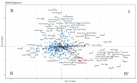
The interpretation of the RGPCA biplot follows the standard geometric principles of PCA-based biplots [22]. The RGPCA biplot divides the districts/cities into four quadrants, which facilitate the interpretation of relative positioning among districts and their association with specific indicators. Districts/cities located in the same direction as an indicator vector are considered to have values above the average. In contrast, those located in the opposite direction of an indicator vector are considered to have values below the average. Meanwhile, districts/cities near the center indicate values close to the average. Based on Figures 5-8, Nduga consistently appears far from the origin (0,0) in the biplot, suggesting that its development profile differs markedly from that of most other districts/cities, which are generally clustered near the center and located in quadrants different from Nduga’s position.
Based on Figure 5, Nduga District is aligned with the direction of the vector representing the indicators of the percentage of households whose sources of drinking water are clean (X1), the percentage of households with sufficient drinking water access (X2), gross participation rate for elementary (X8), junior high (X9) and senior high education (X10). This indicates that Nduga District has relatively high values for these indicators compared to other districts/cities that are not aligned with the direction of these indicator vectors. In the biplot, the relative position of Nduga is close to that of Kepulauan Yapen and Memberamo Tengah. This indicates that the districts of Nduga, Kepulauan Yapen, and Memberamo Tengah had relatively similar human development characteristics in 2019.
Figure 5. A biplot constructed from the 2019 data presents the RGPCA results
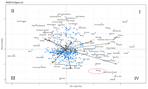
Based on Figure 6, Nduga District is aligned with the direction of the vector representing the indicators of the enrollment rate for children aged 16-18 years (X7), percentage of households whose sources of drinking water are clean (X1) and Average monthly income of workers and employees (X17). This indicates that Nduga District has relatively high values for these indicators compared to other districts/cities that are not aligned with the direction of these indicator vectors. In the biplot, the relative position of Nduga is close to that of Memberamo Tengah, and Maybrat. This indicates that the districts of Nduga, Memberamo Tengah, and Maybrat had relatively similar human development characteristics in 2020.
Figure 6. A biplot constructed from the 2020 data presents the RGPCA results
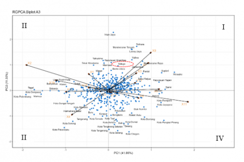
Based on Figure 7, Nduga District is aligned with the direction of the indicator representing the percentage of households without sanitation facilities (X3), marking the emergence of sanitation issues as a new development challenge. Indicators that were previously aligned with Nduga are now positioned farther away, which may reflect a shift in development policy priorities. In the knowledge dimension, the indicators for gross participation rates for junior high education (X9), net participation rates at junior high school (X12) and senrollment rate for children aged 16-18 years (X7) are aligned with Nduga, indicating that Nduga has relatively high values for these indicators. In the biplot, the relative position of Nduga is close to that of Yalimo, suggesting that Nduga and Yalimo had relatively similar human development characteristics in 2021.
Figure 7. A biplot constructed from the 2021 data presents the RGPCA results
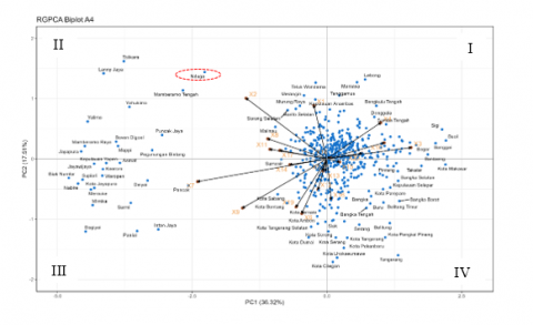
Based on Figure 8, the relative position of Nduga is close to that of Memberamo Tengah. This indicates that Nduga and Memberamo Tengah Districts had relatively similar human development characteristics in 2022. Nduga District is aligned with the direction of the indicators representing Nduga District is aligned with the direction of the indicator representing the percentage of households without sanitation facilities (X3), the percentage of with sufficient drinking water access (X2), gross participation rate for elementary education (X8) and net participation rates at elementary school (X11), and average monthly income of workers and employees (X7). This suggests that these indicators had relatively high values in Nduga.
Figure 8. A biplot constructed from the 2022 data presents the RGPCA results
This study develops Robust Generalized Principal Component Analysis (RGPCA) based on the Euler transformation to address the problem that GPCA is not robust to outliers. The simulation results confirm that the presence of outliers affects the stability of GPCA in determining the dimensions of the reduced matrix, whereas RGPCA preserves the reduced matrix dimensions consistent with the designed cluster structure when outliers are present. These findings demonstrate that integrating the Euler transformation into GPCA improves its robustness while maintaining the simultaneous reduction of row (observation) and column (variable) dimensions.
Human development changes in the Nduga district during 2019-2022 demonstrated fluctuating progress, as shown in the biplot visualization. In 2019, Nduga had relatively high values in the percentage of households whose sources of drinking water are clean, the percentage of households with sufficient drinking water access, and gross participation rate for elementary, junior high, and senior high school education. In 2020, the focus shifted to the enrollment rate for children aged 16-18 years, the average monthly income of workers and employees, and the percentage of households whose sources of drinking water are clean. In 2021, challenges emerged in basic sanitation, as indicated by the high percentage of households without sanitation facilities. However, several indicators in the knowledge dimension still showed relatively high values in Nduga. In 2022, improvements were observed in the percentage of households whose sources of drinking water are clean and sufficient drinking water access, indicating recovery in the Long and Healthy Life dimension. Based on the research findings, dynamic and responsive development planning is needed, with annual monitoring to adjust policy direction in line with the conditions of declining indicators. Similarly, changes in human development across each district/city can be analyzed to identify specific issues in each region. Future studies may focus on the development of GPCA methods for handling missing data, such as through Bayesian Imputation and K-Nearest Neighbors (KNN), as well as exploring the integration of Robust GPCA with these imputation techniques to simultaneously address outliers and missing values
The authors are very grateful to the School of Data Science, Mathematics and Informatics (SSMI), IPB University, for their support. The author also gratefully acknowledges the Indonesian Education Scholarship, the Center for Higher Education Funding and Assessment, and the Indonesian Endowment Fund for Education for support during the doctoral studies.
[1] BPS-Statistics Indonesia. (2020). Human development index 2019. Jakarta: BPS-Statistics Indonesia.
[2] BPS-Statistics Indonesia. (2021). Human development index 2020. Jakarta: BPS-Statistics Indonesia.
[3] BPS-Statistics Indonesia. (2022). Human development index 2021. Jakarta: BPS-Statistics Indonesia.
[4] BPS-Statistics Indonesia. (2023). Human development index 2022. Jakarta: BPS-Statistics Indonesia.
[5] Jollife, I.T., Cadima, J. (2016). Principal component analysis: A review and recent developments. In Philosophical Transactions of the Royal Society A: Mathematical, Physical and Engineering Sciences. 374(2065): 20150202. https://doi.org/10.1098/rsta.2015.0202
[6] Hirari, M., Centofanti, F., Hubert, M., Van Aelst, S. (2025). Robust multilinear principal component analysis. arXiv:2503.07327 . https://doi.org/10.48550/arXiv.2503.07327
[7] Biserka, B., Tatyana, A., Tensor, A.T. (2025). Tensor Decomposition methods for multi-dimensional data analysis. HAL Preprint. https://hal.science/hal-05017799v1.
[8] Li, K., Wu, G. (2021). A randomized generalized low rank approximations of matrices algorithm for high dimensionality reduction and image compression. Numerical Linear Algebra with Applications, 28(1): e2338. https://doi.org/10.1002/nla.2338
[9] Ye, J., Janardan, R., Li, Q. (2004). GPCA: An efficient dimension reduction scheme for image compression and retrieval. KDD '04: Proceedings of the Tenth ACM SIGKDD International Conference on Knowledge Discovery and Data Mining, pp. 354-363. https://doi.org/10.1145/1014052.1014092
[10] Ye, J. (2004). Generalized low rank approximations of matrices. Machine Learning, 61(3): 167-191. https://doi.org/10.1007/s10994-005-3561-6
[11] Ye, J., Janardan, R., Kumar, S. (2011). Biological image analysis via matrix approximation. In Encyclopedia of Data Warehousing and Mining, Second Edition. IGI Global. https://doi.org/10.4018/9781605660103.ch027
[12] Itoh, H., Imiya, A., Sakai, T. (2016). Dimension reduction and construction of feature space for image pattern recognition. Journal of Mathematical Imaging and Vision, 56(1): 1-31. https://doi.org/10.1007/s10851-015-0629-1
[13] Chen, Y., Zhao, Y., He, Y., Xu, F., Jia, W., Lian, J., Zheng, Y. (2019). Face identification with top-push constrained generalized low-rank approximation of matrices. IEEE Access, 7: 160998-161007. https://doi.org/10.1109/ACCESS.2019.2947164
[14] Shi, J., Yang, W., Zheng, X. (2015). Robust generalized low rank approximations of matrices. PLoS One, 10(9): 1-23. https://doi.org/10.1371/journal.pone.0138028
[15] Amini Omam, M., Torkamani-Azar, F. (2016). Noise adjusted version of generalized principal component analysis. Turkish Journal of Electrical Engineering and Computer Sciences, 24(1): 50-60. https://doi.org/10.3906/elk-1303-151
[16] He, L., Yang, Y., Zhang, B. (2023). Robust PCA for high dimensional data based on characteristic transformation. Australia & New Zealand Journal Statistics, 65(1): 127-151. http://doi.org/10.1111/anzs.12385
[17] Johnson, R.A., Wichern, D.W. (2007). Applied Multivariate Statistical Analysis (6th ed.). Pearson Education, Inc.
[18] Harismahyanti, A., Indahwati, Fitrianto, A., Erfiani. (2022). Outlier detection on high dimensional data using minimum vector variance (MVV). Barekeng, 16(3): 797-804. https://doi.org/10.30598/barekengvol16iss3pp797-804
[19] Fitrianto, A., Xin, S.H. (2022). Comparisons between robust regression approaches in the presence of outliers and high leverage points. BAREKENG: Jurnal Ilmu Matematika dan Terapan, 16(1): 243-252. https://doi.org/10.30598/barekengvol16iss1pp241-250
[20] Liwicki, S., Tzimiropoulos, G., Zafeiriou, S., Pantic, M. (2013). Euler principal component analysis. International Journal of Computer Vision, 101(3): 498-518. https://doi.org/10.1007/s11263-012-0558-z
[21] Yan, W., Tinker, N.A. (2006). Biplot analysis of multi-environment trial data: Principles and applications. Canadian Journal of Plant Science, 86(3): 623-645. https://doi.org/10.4141/P05-169
[22] Engloner, A.I., Podani, J. (2023). A new statistical method for the comparison of biplots with the same objects and variables. Ecological Indicators, 154: 110802. https://doi.org/10.1016/j.ecolind.2023.110802
[23] Saeidnia, F., Taherian, M., Nazeri, S.M. (2023). Graphical analysis of multi-environmental trials for wheat grain yield based on GGE-biplot analysis under diverse sowing dates. BMC Plant Biology, 23(1): 198. https://doi.org/10.1186/s12870-023-04197-9
[24] Nariswari, R., Prakoso, T.S., Hafiz, N., Pudjihastuti, H. (2022). Biplot analysis: A study of the change of customer behaviour on e-commerce. Procedia Computer Science, 216: 524-530. https://doi.org/10.1016/j.procs.2022.12.165
[25] Ahmadi, S., Rezghi, M. (2020). Generalized low-rank approximation of matrices based on multiple transformation Pairs. Pattern Recognition, 108: 107545. https://doi.org/10.1016/j.patcog.2020.107545