Rihab Hazim Qasim*![]() | Sura Mahroos Searan
| Sura Mahroos Searan![]() | Yaqeen Saad Ali
| Yaqeen Saad Ali![]() | Nadia Fahad
| Nadia Fahad![]()
© 2025 The authors. This article is published by IIETA and is licensed under the CC BY 4.0 license (http://creativecommons.org/licenses/by/4.0/).
OPEN ACCESS
The grape industry’s economic and social importance has fostered the advancement of cutting-edge technologies for the live tracking of vineyards, aiming to enhance the quality of the fruit. The recent advancement of computer vision algorithms and the preparation of new image sensors has made it possible to automate the identification of grapevine varieties. Classifying grape varieties based on their kinds using images is a challenging operation that necessitates the extraction of numerous distinguishing traits. In this paper, we proposed a technique for detecting and separating clusters of grapes in a field and subsequently categorizing them into eight different types applying convolutional neural network (CNN) models and the hyper-parameters tuned to each classification algorithm. This paper used a public data set of 8000 images in eight categories (1000 images per category). The proposed CNN model exceeded existing grape leaf classification work borrowed from the dataset, reaching 100% training accuracy, and experimental results showed the certainty of the proposed classification method at 60% testing accuracy.
pattern recognition, grape’s type, image classification, hyperparameter tuning, CNN
Digital Agriculture (DA) in recent years exponential rise in the total of data created by agricultural go per hectare. In precision viticulture and site-specific management in viticulture have expanded the information available to winegrowers [1]. The industry of grape economic and social importance has fostered the advancement of cutting-edge technologies for the live tracking of vineyards, aiming to enhance the quality of the fruit. As an effect, there is need to do accurate techniques for find and verifying grape varieties, specifically when it comes to selling vine cuttings to vineyards, detecting forbidden species or varieties in specific regions, or estimating the market value of different grape varieties in various production areas [2].
The development of an automatic algorithm for identifying grape varieties based on leaves faces many challenges. Ampelography is the specific discipline of botany that deals with identifying and differentiating different grape varieties [3, 4]. The factors that have been briefly outlined share a common requirement: the presence of a skilled specialist at the grape picking location, who must directly deal with the actual fruit. The agricultural regions are predicted to be substantial, but providing a constant presence of experts is impossible. Hence, it is desirable to automate the process of grape detection by utilizing drones equipped with cameras, for instance. Nevertheless, drones lack the intuitive abilities of professionals and not equipped with organoleptic sensors. Performing a DNA test is the most dependable method for identifying a grape variety. However, it is also challenging to envision integrating a DNA test kit into agricultural equipment [5]. Nonetheless, the utilization of specialist software necessitates the participation of a highly trained expert [6]. The efficacy of this approach is heavily contingent upon the proficiency and expertise of the specialist. A more objective approach, such as DNA analysis [7], is available. However, this process, along with other wet chemical techniques, is damaging, time-consuming, labor-intensive, and necessitates the expertise of a specialist. Recent advances in computer vision algorithms so the availability of new imaging sensors that led to the automated identification of grape varieties. The processing of data from a spectrometer [8, 9] or a high-spectral camera is automated non- invasive and rapid. Accurate identification of grapevine types can be achieved by measuring the interaction between electro- magnetic radiation and matter across various spectral bands. An inherent drawback of this method is the substantial cost of acquiring a spectrometer nor hyperspectral camera, that be significantly greater by many orders of magnitude when compared to a standard camera. Incorporating these sensors into a specialized harvester would substantially raise its cost. Human sensory capabilities constrain conventional approaches for identifying grapevine varietals. For instance, amperometry uses visual perception to identify different grapevine varieties. The classification of grapevines based on their kinds using images is a challenging operation that necessitates the extraction of numerous distinguishing traits. The wide range of elements in an out- side environment adds to the difficulty of extracting specific features [10]. In this paper the dataset that use has eight folders include 8000 images in eight categories (1000 images per category) each representing a specific grape variety, with every file containing 1000 images in JPG format. All the pictures in the collection have a 6000 × 4000 pixels resolution Figure 1 [11].
Figure 1. Examples of each grape classes [11]
Grapes have various physical, chemical, and geographical properties that affect their health. Moreover, different varieties of the same plants in the same region can also have different yields depending on growth stages or grape quality. Consequently, various stages of growth require different monitoring. Therefore, it is essential to distinguish between wine varieties produced in the same region, and the relationship between varieties and the development of certain substances is a crucial factor to be recognized. This paper aims to detect and analyze several varieties of vineyards by their spectral properties. The results of this correlation will lead to the creation of a vineyard map. Knowing the specific locations of each variety helps farmers avoid errors and ensures the quality of each variety. The objective is to implement the classification methods of varieties with common characteristics to ensure efficient management of different varieties in the same region. In addition to visible (RGB), multispectral images include red edges and near- infrared regions of the spectrum, which are not always visible to the naked eye. The scope of this methodology is to inform farmers about the specific characteristics of grape varieties; this information can be invaluable to vineyard management when planning, cutting, fertilizing, and harvesting during its lifetime. For this task, we proposed the CNN , and the hyperparameters were tuned for every classification algorithm. A change was made to the hyperparameter to verify its accuracy CNN consists of convolutional, pooling, and fully connected layers. The purpose of these layers in the CNN is to generate complex features that enhance classification effectiveness. The convolutional layers in this study comprise a collection of feature maps. Contributions of this research are as follows: Grape varieties with similar characteristics can be clustered using a combination of vegetation on the data set. Random splitting dataset in to training, testing and validation to development of robust and valid model. Automatic recognition of grapevine varieties using of deep learning by design the best model for the grapevine varieties automatic identification.
The residue of this paper as follows: Section 2 involves related work that handles the same problem and explain how other works solved it. In Section 3, we present CNN model, and the hyperparameters were tuned for every classification algorithm. Section 4 explains results and discuss the result. Lastly, Section 5 gives the conclusion and future models.
There is a wealth of research on identifying grapevine varieties, the image categorization systems considered the most advanced that are built using deep convolutional networks. This work [12] proposed three models for detecting and separating clusters of grapes in a field and subsequently categorizing them into five different types using KSM, ResNet, and ExtResNet models. This study [13] proposed a basis for applying the used cases, such as identifying diseases exclusive to specific types or unique fungal diseases. Contemporary network topologies regulate capacity by adjusting the breadth or depth of networks. Expanding the space of a deep ConvNet by extending width is employed, for example, an alternative method is to augment the number of network layers known as the grid deepness while maintaining the linearity of data image processing [14].
Various network architectures, like Highway Networks [15] proposed the model of neural networks is important for this model. Introduce an architecture design our so-called highway networks allow to pass data at many layers on data highways. They are same by LSTM and allow the data pass using adaptive gats item. Deep Pyramidal Residual Networks [16] proposed deep convolutional neural networks (DCNNs) had been seen great implementation in image categorization labor in last years. Normally, deep neural network flowcharts are load depend of a large set of layers, and they do down sampling on the spatial dimension to reduce memory usage using by collect. Simultaneously, the element map size (i.e., the number of channels) is clear better at down sampling place, that is key to make sure useful show. This study [17] presented a Dense Convolutional Network (DenseNet) that link all layer to each last layer in a feed-forward mode. while set convolutional networks with L layers had L connections one between all layer and its next layer us network has L(L+1)2direct links. This study [18] presented the cross-layer neurons design a new structure with deep neural network training capability. It makes use of cross-layer neurons to post data (features) acquired from all of the lower-level layers to the higher-level layers. The work by Pereira et al. [3] devised a technique to automatically detect grape bunches in color photographs. A trained ConvNet was utilized to segment the image.
The data was classified into a limited number of specific categories and compared with sub-regions of known dimensions. The grape group pixel by pixel was segmentation to do using probability plot for each category. The segmentation of grape clusters in-range photos achieved an accuracy of 87.5%. Franczyk et al. [12] presented an approach that used a KSM a restnet and an ExtRestnet to recognize and divide clusters of grapes in a crop in order to categorize five different types of grapes from a provided image dataset. Mohimont et al. [19] introduced a total analysis available to each overall non-expert readers to compare the new going of artificial intelligence (AI) in viticulture. Finally, Palacios et al. [20] presented an architecture using SegNet that working to discover the seen grain and cover attribute. All attribute that used to train models support vector regression (SVR) for predict number of real berries and heed.
Our research’s primary objective is to accurately identify grape varieties using only the image of the grape being displayed. For this task we proposed the CNN and the hyperparameters were tuned for every classification algorithm. A change was made to the hyperparameter to verify its accuracy. Figure 2 shows the flowchart of this proposed method.
Figure 2. Flowchart of the proposed methodology
3.1 Dataset
The dataset has eight folders include 8000 images in eight categories (1000 images per category) each representing a specific grape variety, with each folder containing 1000 images in JPG format. All the pictures in the collection have a 6000 × 4000 pixels resolution. Due to the photographs’ high resolution, their size reached 49.8 GB, which is impractical for downloading and uploading the dataset from the Internet. To address this issue, the images were resized using a Windows application called (resize pictures) to the proportions of 1620 × 1080 pixels. The initial data size is 1.95 gigabytes. Compression using a zip application reduced the data size to 1.83 gigabytes. Eight folders represent different grape variety types (Deas Al- Annz, Kamali, Halawani, Thompson Seedless, aswud balad, riasi, frinsi, and shdah).
$X_{ {normalized }}=\frac{X-X_{min }}{X_{max }-X_{min }}$ (1)
3.1 Dataset
a) Batch Size and Selection: Before commencing the training process, batch size is one of the primary hyperparameters that necessitates adjustment. The batch size is a reference to the quantity of images used in the gradient estimation procedure. Several studies have examined the impact of batch size on network performance, specifically in terms of accuracy and convergence time. The objective was to establish whether small or large batches were more advantageous. While a small batch size may converge more quickly than a big batch, the major batch size has the likely to reach best minima that a smaller batch size cannot achieve. Also, a small batch size might induce real regularization due to its elevated variance [21]. In this work on image classification, we empirically utilize a batch size of 32.
b) Convolutional neural networks (CNNs): CNN consists of convolutional, pooling, and fully connected layers. The purpose of these layers in the CNN is to generate complex features that enhance classification effectiveness. The convolutional layers in this study comprise a collection of feature maps. Each feature map has a receptive field that covers only a small part of the input spectra. Each feature map generated results from performing a convolution (dot product) between the weights of the receptive field and all the points in the spectrum. This indicates that adjacent points in the feature map were identified in overlapping and adjoining portions of the input spectra. In this manner, several characteristics are identified across the entire spectra range. One significant benefit of employing convolutional layers is their much- reduced number of trainable parameters compared to a fully connected neural network. The pooling layer is utilized on the feature maps to achieve down-sampling. In this scenario, the feature maps were partitioned into distinct regions that do not overlap, and the highest value within each region was selected. Subsequently, dropout is implemented where training certain elements that contribute to the subsequent layer are either excluded or included with a specific probability. Following the convolution and pooling layers, which consist of one of each in this study. Fully connected neural network analyzes the features derived from the preceding layers. Applies a flattened layer to a Keras model. The flattened layer transforms the input from a multidimensional array to a one-dimensional one. This is frequently performed when converting from a convolutional layer to a fully linked layer.
Pooling: Reducing the size of the map at the final layer of the deep network enhances its suitability for classification tasks we use. Including a pooling layer ensures that slight variations in input images do not affect the output while also decreasing the dimensions of the feature maps, such as width and height. A nonlinear function f() was applied element-wise to c: a for every feature map c. The activations obtained, represented by the letter a, were then sent to the MaxPooling2D layer is standard in convolutional neural networks [22]. It reduces the output’s spatial dimensions, which can enhance the model’s execution by lowering the number of account and parameters [23].
c) Learning rate and Dropout: for regularization the learning rate is a critical parameter in CNN that determines the speed at which a network adjusts its parameters during backpropagation [24]. Reducing the learning rate promotes gradual pool but also hampers the process speed learning. Nevertheless, maintaining a higher learning rate can accelerate the learning process, but it may impede convergence. Dropout is an effective and uncomplicated regularization method for deep learning models [25], and convolutional neural networks (CNNs) often tend to overfit. Co-adaptation is more likely to occur when a fully connected layer contains numerous nodes or neurons [26]. This approach randomly picks neurons and excludes them throughout the training phase eliminating their impact on subsequent processes.
Table 1. The configuration of the model CNN
|
Output Shape |
Type |
Layer |
|
(28, 28, 32) (14, 14, 32) (14, 14, 32) (12, 12, 64) (6, 6, 64) (6, 6, 64) (4, 4, 128) (2, 2, 128) (2, 2, 128) (2, 2, 256) (2, 2, 256) (2, 2, 256) 512 64 64 64 num_classes |
32 filters, (3, 3), ReLU (2, 2) - 64 filters, (3, 3), ReLU (2, 2) - 128 filters, (3, 3), ReLU (2, 2) - 256 filters, (3, 3), ReLU (2, 2) - - 64 neurons, ReLU dropout_rate - num_classes neurons, softmax |
Conv2D MaxPooling2D BatchNormalization Conv2D MaxPooling2D BatchNormalization Conv2D MaxPooling2D BatchNormalization Conv2D MaxPooling2D BatchNormalization Flatten Dense Dropout BatchNormalization Dense |
d) Batch normalization and L2 regularization: Batch normalization is a further regularization technique that standardizes the collection of activations in a layer. Normalization is achieved by subtracting the mean of the batch from each activated and then using the standard deviation and dividing the batch. Normalization, in conjunction with standardization is a commonly used method in preprocessing pixel values. Conventional L2 regularization is applied to all trainable parameters, meaning the regularization factors remain constant during training. Addition is the mathematical operation of combining two or more numbers to find their total sum. Indeed, the selection of those regularization factors must be done manually through hyperparameter optimization [27]. Table 1 shows the configuration of the best model.
Model hyperparameter optimization strategy following the establishment of a CNN backbone architecture and specific hyperparameters learning rate and Dropout rates to achieve the most outstanding performance (accuracy, loss, etc.). These adjustments are necessary to ascertain the optimal model of this CNN to fit the training and validation dataset. Algorithm 1hyperparameter tuning by systematically trying different combinations of learning rates and dropout rates and selecting the best-performing model.
$Accuracy$ $=\frac{T P+T N}{T P+T N+F N+F P}$ (2)
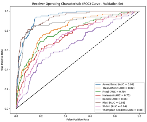
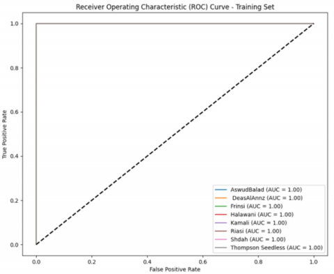
Figure 3. ROC classification model
|
Algorithm 1: hyperparameter tuning |
|
Inputs: Learning rates to tune: [0.0001, 0.001, 0.01] Dropout rates to tune: [0.2, 0.5, 0.7] |
|
Output: Print the best hyper parameters (learning rate and dropout rate) and best accuracy. |
|
In this study a CNN network was investigated. The model was trained on 6400 images, divided into a training set of 80%, a validation set of 10%, and a testing set of 10%. The LR range test is a method for finding the optimal learning rate for a CNN. The test starts with a small learning rate and slowly increases it linearly. This provides information on how well the network can be trained over various learning rates. When the learning rate is too small, the network will not converge. The network will overfit the training data when the learning rate is too large. The optimal learning rate is the point at which the network converges without overfitting. This study used the LR range test to find the optimal learning rate for the CNN. The train found the optimal learning rate was 0.0001, depending on validation accuracy. This learning rate was used to train the network, and the network achieved a high accuracy on the testing set. The following Table 2 shows validating details and hyperparameters, Table 3 shows final train, validation and test accuracy.
Table 2. Validating details and hyperparameters.
|
Learning Rate |
Dropout Rate |
Validation Accuracy |
|
0.0001 |
0.2 |
%46 |
|
0.0001 |
0.5 |
%37 |
|
0.0001 |
0.7 |
%34 |
|
0.001 |
0.2 |
%28 |
Table 3. Final train validation and test accuracy.
|
Learning Rate |
Dropout Rate |
Epoch |
Train |
Validation Accuracy |
Testing_ Accuracy |
|
0.0001 |
0.2 |
20 |
100% |
43% |
60% |
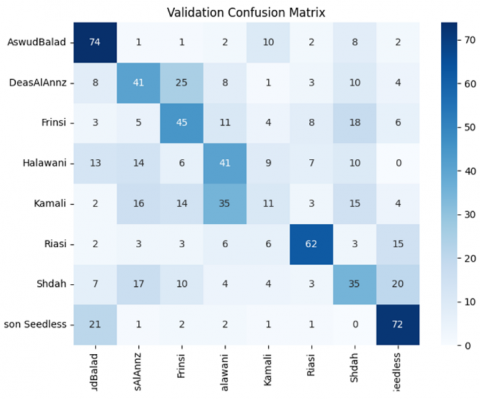
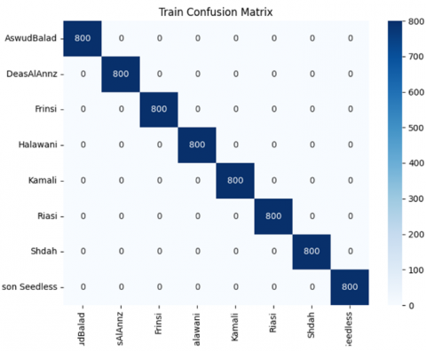
Figure 4. Confusion matrix classification model
In the classification of species varieties, the similarities and differences between the classes are high, placing the task in the family of delicate recognition problems. In the images obtained on the field there is a wide number of unrelated information, which can contribute to classification errors. Another factor to pay attention to is the natural existence of tailed classes in datasets since this task can be treated as a long-tailed data distribution classification. Imbalance can be problematic because the model tends to overfit the courses with more samples. In this context, few-shot learning approaches can be applied to minimize the lack of samples for some categories. This paper tested the use of focal loss to deal with unbalance in the dataset, even if there were no tail classes. Other balanced losses can still be tested in the dataset (between 60 and 75 images per category). Introducing the Softmax is class-Balanced cross-entropy loss. The reduction of the cross-entropy loss that start a weighting factor is backward relative to the suitable number of samples in a category. Created a loss function using an effect rate to identify how each sample affects biased decisions that cause the model to overfit. They fix weights to each sample accordingly. model's overall categorization test performance. This curve contains the true positive rate (TPR) and false positive rate (FPR), with specificity FPR = −1.
A thorough examination of the system's implementation using up confusion matrix Figure 4 reveals it while the model does a good job of differentiating across grape varieties, it performs poorly when it comes to types 4, 5 and 7. This occur because the similarities and differences between the classes are high, placing the task in the family of delicate recognition problems. In the images obtained on the field there is a wide number of unrelated information, which can contribute to classification errors. Only grapes with similar shapes become confused.
The classification of grape vines using advanced computer vision techniques represents a significant advancement in the grape industry. By automating the identification process and enabling live tracking of vineyards, this technology can revolutionize crop management and improve the quality of grapes. The proposed CNN model, with its impressive training and testing accuracy, demonstrates the feasibility and effectiveness of this approach. As research in this field progresses, we can expect to see even more sophisticated and accurate classification systems that benefit both grape growers and consumers. The present research employs a transfer learning strategy based on the CNN architecture. It was demonstrated to automatically recognize and categorize eight different types of grapes from a provided image dataset. The CNN Classification successfully trained on correctly detected type of grapes, achieving 100% accuracy. With a 60% testing accuracy, the experimental findings showed the suggested classifier's dependability. In the future work, the hyperparameters of the CNN model will be optimized to achieve better classification accuracy and eliminate the high complexity in the models.
We want to pass our sincere thanks to each our colleagues, whose significant contributions and valuable feedback have greatly enriched this research. Their collaborative efforts and insights have been instrumental in completing this work.
[1] Sozzi, M., Cantalamessa, S., Cogato, A., Kayad, A., Marinello, F. (2022). Automatic bunch detection in white grape varieties using YOLOv3, YOLOv4, and YOLOv5 deep learning algorithms. Agronomy, 12(2): 319. https://doi.org/10.3390/agronomy12020319
[2] Diago, M.P., Fernandes, A.M., Millan, B., Tardaguila, J., Melo Pinto, P. (2013). Identification of grapevine varieties using leaf spectroscopy and partial least squares. Computers and Electronics in Agriculture, 99: 7-13. https://doi.org/10.1016/j.compag.2013.08.021
[3] Pereira, C.S., Morais, R., Reis, M.J.C.S. (2019). Deep learning techniques for grape plant species identification in natural images. Sensors, 19(22): 4850. https://doi.org/10.3390/s19224850
[4] Nuske, S., Achar, S., Bates, T., Narasimhan, S., Singh, S. (2011). Yield estimation in vineyards by visual grape detection. In Proceedings of the 2011 IEEE/RSJ International Conference on Intelligent Robots and Systems (IROS 2011), Francisco, CA, USA, pp. 2352-2358. https://doi.org/10.1109/IROS.2011.6048830
[5] Gupta, M., Chyi, Y.S., Romero‑Severson, J., Owen, J.L. (1994). Amplification of DNA markers from evolutionarily diverse genomes using single primers of simple‑sequence repeats. Theoretical and Applied Genetics, 89(7): 998-1006. https://doi.org/10.1007/BF00224530
[6] Soldavini, C., Stefanini, M., Dallaserra, M., Policarpo, M., Schneider, A. (2009). SUPERAMPELO, a software for ampelometric and ampelographic descriptions in Vitis. Acta Horticulturae, 827: 253-258. https://doi.org/10.17660/ActaHortic.2009.827.43
[7] Pelsy, F., Hocquigny, S., Moncada, X., Barbeau, G., Forget, D., Hinrichsen, P., Merdinoglu, D. (2010). An extensive study of the genetic diversity within seven French wine grape variety collections. Theoretical and Applied Genetics, 120(6): 1219-1231. https://doi.org/10.1007/s00122-009-1250-8
[8] Gutiérrez, S., Tardaguila, J., Fernández‑Novales, J., Diago, M.P. (2016). Data mining and nir spectroscopy in viticulture: Applications for plant phenotyping under field conditions. Sensors, 16(2): 236. https://doi.org/10.3390/s16020236
[9] Fernandes, A., Utkin, A., Eiras‑Dias, J., Silvestre, J., Cunha, J., Melo‑Pinto, P. (2018). Assessment of grapevine variety discrimination using stem hyperspectral data and AdaBoost of random weight neural networks. Applied Soft Computing, 72: 140-155. https://doi.org/10.1016/j.asoc.2018.07.059
[10] Gutiérrez, S., Fernández‑Novales, J., Diago, M.P., Tardaguila, J. (2018). On‑The‑Go hyperspectral imaging under field conditions and machine learning for the classification of grapevine varieties. Frontiers in Plant Science, 9: 1102. https://doi.org/10.3389/fpls.2018.01102
[11] Al-Khazraji, L.R., Mohammed, M.A., Abd, D.H., Khan, W., Khan, B., Hussain, A.J. (2023). Image dataset of important grape varieties in the commercial and consumer market. Data Brief, 47: 108906. https://doi.org/10.1016/j.dib.2023.108906
[12] Franczyk, B., Hernes, M., Kozierkiewicz, A., Kozina, A., Pietranik, M., Roemer, I., Schieck, M. (2020). Deep learning for grape variety recognition. Procedia Computer Science, 176: 1211-1220. https://doi.org/10.1016/j.procs.2020.09.117
[13] Krizhevsky, A., Sutskever, I., Hinton, G.E. (2017). Imagenet classification with deep convolutional neural networks. Communications of the ACM, 60(6): 84-90. https://doi.org/10.1145/3065386
[14] Szegedy, C., Vanhoucke, V., Ioffe, S., Shlens, J., Wojna, Z. (2016). Rethinking the inception architecture for computer vision. In Proceedings of the IEEE Conference on Computer Vision and Pattern Recognition (CVPR 2016), pp. 2818-2826. https://doi.org/10.1109/CVPR.2016.308
[15] Srivastava, R.K., Greff, K., Schmidhuber, J. (2015). Training very deep networks. In Proceedings of the 28th International Conference on Neural Information Processing Systems (NIPS 2015), Cambridge, MA, USA, pp. 2377-2385. https://doi.org/10.48550/arXiv.1507.06228
[16] Han, D., Kim, J., Kim, J. (2017). Deep pyramidal residual networks. In Proceedings of the 2017 IEEE Conference on Computer Vision and Pattern Recognition (CVPR 2017), pp. 6307-6315. https://doi.org/10.1109/CVPR.2017.668
[17] Huang, G., Liu, Z., van der Maaten, L., Weinberger, K.Q. (2017). Densely connected convolutional networks. In Proceedings of the IEEE Conference on Computer Vision and Pattern Recognition (CVPR 2017), Honolulu, HI, USA, pp. 2261-2269. https://doi.org/10.1109/CVPR.2017.243
[18] Yu, Z., Li, T., Luo, G., Fujita, H., Yu, N., Pan, Y. (2018). Convolutional networks with cross layer neurons for image recognition. Information Sciences, 433: 241-254. https://doi.org/10.1016/j.ins.2017.12.045
[19] Mohimont, L., Alin, F., Rondeau, M., Gaveau, N., Steffenel, L.A. (2022). Computer vision and deep learning for precision viticulture. Agronomy, 12(10): 2463. https://doi.org/10.3390/agronomy12102463
[20] Palacios, F., Diago, M.P., Melo-Pinto, P., Tardáguila, J. (2022). Early yield prediction in different grapevine varieties using computer vision and machine learning. Precision Agriculture, 24(2): 407-435. https://doi.org/10.1007/s11119-022-09950-y
[21] Wilson, D.R., Martinez, T.R. (2003). The general inefficiency of batch training for gradient descent learning. Neural Networks, 16(10): 1429-1451. https://doi.org/10.1016/S0893-6080(03)00138-2
[22] Zeiler, M.D., Fergus, R. (2013). Stochastic pooling for regularization of deep convolutional neural networks. arXiv 2013. arXiv preprint arXiv: 1301.3557. https://doi.org/10.48550/arXiv.1301.3557
[23] Singh, P., Manure, A. (2019). Introduction to tensorflow 2.0. In Learn TensorFlow 2.0: Implement Machine Learning and Deep Learning Models with Python, pp. 1-24. https://doi.org/10.1007/978-1-4842-5558-2
[24] Yeh, W.C., Lin, Y.P., Liang, Y.C., Lai, C.M., Huang, C.L. (2023). Simplified swarm optimization for hyperparameters of convolutional neural networks. Computers and Industrial Engineering, 177: 109076. https://doi.org/10.1016/j.cie.2023.109076
[25] Srivastava, N., Hinton, G., Krizhevsky, A., Sutskever, I., Salakhutdinov, R. (2014). Dropout: A simple way to prevent neural networks from overfitting. Journal of Machine Learning Research, 15(1): 1929-1958. http://jmlr.org/papers/volume15/srivastava14a/srivastava14a.pdf.
[26] Adrian, G. (2018). Dropout in Recurrent Neural Networks. https://adriangcoder.medium.com/a-review-of-dropout-as-applied-to-rnns-72e79ecd5b7b.
[27] Ni, X., Fang, L., Huttunen, H. (2021). Adaptive L2 regularization in person re-identification. In 2020 25th International Conference on Pattern Recognition (ICPR), pp. 9601-9607. https://doi.org/10.1109/ICPR48806.2021.9412481
[28] Manai, E., Mejri, M., Fattahi, J. (2024). Confusion matrix explainability to improve model performance: application to network intrusion detection. In 2024 10th International Conference on Control, Decision and Information Technologies (CoDIT), Vallette, Malta, pp. 1-5. https://doi.org/10.1109/codit62066.2024.10708595
[29] Qasim, R.H., Al‑Ani, M.S. (2018). Efficient approach of detection and visualization of the damaged tablets. Journal of Theoretical and Applied Information Technology, 96(3): 643-656.
[30] Bianco, A.M., Boente, G., Gonzalez-Manteiga, W. (2020). A robust approach for ROC curves with covariates. arXiv preprint arXiv: 2007.00150. https://doi.org/10.48550/arXiv.2007.00150