Hanan Magroun*![]() | Smaine Mazouzi
| Smaine Mazouzi![]() | Hamid Serdi
| Hamid Serdi![]()
© 2025 The authors. This article is published by IIETA and is licensed under the CC BY 4.0 license (http://creativecommons.org/licenses/by/4.0/).
OPEN ACCESS
Digital image analysis requires segmentation to distinguish regions of interest. This step is vital in medical imaging, particularly in oncology, for tumor detection and localization, assisting doctors and surgeons in performing timely interventions. While graph cut methods are effective, their reliance on manual seed initialization limits reproducibility and clinical utility. This paper introduces a fully automated graph cut framework to address this limitation. The method processes co-registered FLAIR and T1-weighted images from the TCIA Brain-Tumor-Progression dataset. Preprocessing involves skull stripping, median filtering, and contrast enhancement. Segmentation starts with the ICM algorithm extracting edema from FLAIR images, which then guides multi-scale FCM to generate probability maps distinguishing object and background pixels. These pixels serve as initial seeds for automated graph cut segmentation on T1-weighted images, delineating the tumor region. Post-processing refines results using FCM clustering. Quantitative evaluation on 20 patient cases achieved values of 0.96 for specificity, 0.98 for sensitivity, 0.99 for NPV, 0.98 for PPV, and 0.99 for accuracy, and a mean Dice coefficient of 0.89 ± 0.02 for tumor segmentation, outperforming the interactive graph cut baseline (0.80 ± 0.05) by 9%. This fully automated framework provides robust, accurate segmentation without operator dependence, making it suitable for clinical use.
brain tumor segmentation, multimodal MRI, graph cut, seed initialization, ICM algorithm, edema segmentation, skull tripping, multi-scale FCM
Correct determination of the volume of brain tumor parts is crucial for tracking evolution, organizing radiation therapy, assessing results, and conducting follow-up investigations. Therefore, precise delimitation of tumors is required [1]. Glioma is one of the deadliest primary brain tumors owing to its poor chance of survival [2]. In this context, the World Health Organization (WHO) has divided cerebral gliomas into four groups based on their severity: grades 1 and 2 are considered Low-Grade Gliomas (LGG) because of their slow-growing nature, while grades 3 and 4 are considered severe and High-Grade Gliomas (HGG) [3].
Accurate demarcation of gliomas plays a crucial role in the diagnosis, treatment planning, and evaluation of treatment outcomes. Nevertheless, manual delineation is subject to inaccuracies and is a labor-intensive process that can lead to discrepancies between observers. Therefore, automated delineation methods are required to enhance the accuracy and efficiency of this process. However, automating glioma delineation remains challenging because of heterogeneity in the shape, size, and location of gliomas [4-6].
Advancements in image processing have contributed significantly to the detection of brain tumors. Magnetic Resonance Imaging (MRI) is a common technique used to obtain brain images [7]. An MRI scan includes four imaging modalities: T1-weighted (T1), T2-weighted (T2), T1-withcontrast- enhanced (T1-w), and fluid-attenuated inversion recovery (FLAIR). These modalities provide additional information for assessing brain tumor subregions, especially in gliomas [8, 9].
For many years up to the present day, technologies related to the acquisition and visualization of MR images have continued to evolve, this progress has always been accompanied by the emergence of new brain MRI segmentation methods and frameworks. Owing to their robustness, graph-based methods have been widely used to segment medical images, particularly MR images. Some of them [10-13] revolve around the basic idea of extracting features specific to each modality and then integrating them to construct a fused and unified graph that accomplishes segmentation. Others [14-16] are commonly utilized in cascade architectures by many individuals, where graph entries are generated in the preceding stages, creating a sequential flow of information through the graph. These methods allow for a structured and efficient process of utilizing graph cuts to achieve the desired outcomes. Currently, efforts are being directed towards using deep neural networks to predict the energy parameters of graph cuts to benefit from the power of deep learning and improve the performance of multimodal image segmentation [17].
Most existing multimodal image segmentation approaches using graph cuts suffer from a critical limitation: they require manual or semi-automated seed initialization [18-20]. While interactive approaches are accurate, they introduce operator dependency, making the process time-consuming and unsuitable for reproducible large-scale clinical application. Previous attempts at automation using simple heuristics or intensity thresholding [21] often lack robustness when dealing with the complex intensity profiles of brain tumors evident in multimodal MRI. This persistent need for manual intervention or non-robust automation is a significant bottleneck.
In this work, we address this gap by introducing a novel initialization pipeline that capitalizes on the theoretical strengths of graph cut while removing user dependency, thus ensuring truly automated and reproducible segmentation. Our main contribution is the introduction of a new graph-cut-based framework for fully automated brain tumor segmentation from multimodal MR images, specifically the Flair and T1-w modalities. This framework automatically selects the background and tumor seeds without user intervention, primarily to identify two distinct segments: edema and tumor. The remainder of this paper is organized as follows: Section 2 presents top studies that have dealt with the segmentation of multimodal MR images. The proposed fully automated framework is described in Section 3. Section 4 presents the results of the segmentation. An interpretation of the results of our study and a comparison with existing research is presented to highlight their importance. Finally, Section 5 provides an overview of the contribution of this study and highlights its future perspectives.
For several decades, to provide efficient vision models and frameworks, many authors have proposed different methods for the segmentation of multimodal MRI. Among the first significant works published is a paper that relied heavily on Random Forest (RF) classification, marking an important milestone in this research area. In this context, a fully automatic brain tumor segmentation technique was suggested by Bauer et al. [22], where the segmentation task was modeled as a conditional random field by energy minimization formulation followed by random forest-based classification. The authors obtained encouraging results for the BraTS2012 dataset. Zikic et al. [23] then combined initial tissue probabilities evaluated by a parametric based on Gaussian Mixture Model (GMM) and Forest-based classification in an automatic framework. Tustison et al. [24] applied a two stages based framework for tumor segmentation, where the aim of the first stage was to generate features images. They then constructed a Random Forest model and probability images. Subsequently, Reza and Iftekharuddin [25] proposed fully automated multiclass abnormal brain tissue segmentation based on classical random forest-based classification of extracted image features.
Since 2014, Convolutional Neural Networks (CNN) have increasingly dominated the field of medical imaging, as demonstrated by contributions to brain tumor multimodal segmentation and BraTS challenge submissions [26, 27]. As a sample, Urban et al. [28] proposed a CNN in which a tiny 3D patch for each input channel was employed to offer local data and establish predictions. Zikic et al. [29] also modified a conventional CNN implementation based on multichannel 2D convolutions to work on multimodal 3D MRI. Havaei et al. [30] developed a 2D CNN-based model with a cascaded architecture that simulated the local dependency of labels, in which two parallel CNNs were utilized to extract the local or global context of the tissue appearance of the input patches. In the study [31], the authors separated the segmentation issue into three independent binary segmentation sub-tasks, and a CNN was fed the 2D image feature patches for each sub-task to predict which label patches would most likely be present in the center of each image patch. Kamnitsas et al. [32] used DeepMedic, a 3D CNN architecture that has previously been introduced in the study [1]. DeepMedic is an 11-layer 3D CNN with lingering connections. Wang et al. [33] presented a cascade of fully convolutional neural networks. The cascade is designed to break down multiclass segmentation into a string of three binary segmentations in accordance with the hierarchy of subregions. SegNet, a technique built on a two-dimensional convolutional neural network, was used by Yang et al. [34] to create autonomous segmentation of brain tumors. The authors contrasted workout plans that included and did not include slices without well-defined tumor locations, and where MR images were processed according to the Flair modality.
With an asymmetrically big encoder to extract deep features from the image and a decoder portion that reconstructs dense segmentation masks, Myronenko [35] suggested a semantic segmentation network of tumor subregions from 3D MRI for BraTS 2018 challenge, where they win first place.
More recently, researchers have turned their attention to transformer models. SwinBTS proposed by Jiang et al. [36] integrates Swin Transformers with CNN-based encoder-decoder structures. These hybrid approaches achieve superior results in terms of segmentation accuracy and robustness on multimodal datasets. More recently, Liu et al. [37] proposed M3AE, a multimodal representation learning framework designed to handle missing modalities in brain tumor segmentation. Following this review of the most common works in the field of tumor segmentation from multimodal MRI, we conclude that there is not much research on the use of the graph cut technique within the above-mentioned field. The majority of tumor segmentation techniques are based on either machine learning or deep learning approaches.
Despite the advancements in brain tumor segmentation discussed in the literature, challenges such as the need for manual intervention and the difficulty in accurately segmenting tumors due to their heterogeneity persist. Our proposed framework aims to address these challenges by introducing a fully automated graph cut-based segmentation process, as detailed in the following sections.
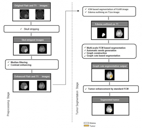
The framework begins with preprocessing using Flair and T1 modalities, performing skull stripping to separate the membrane from the skull, followed by median filtering and contrast enhancement to improve image quality. The second stage focuses on tumor delineation from the T1 image, starting with edema pre-segmentation from the Flair image using the ICM algorithm. Next, the edema mask is applied to the T1 image for Multi-scale FCM processing, generating probability maps that serve as initial seeds for graph cut. The region extracted from the T1 image was then automatically segmented using Graph Cut to separate the tumor from edema.
Finally, standard FCM clustering smoothes the boundaries of the tumor region, producing a well-defined output. Figure 1 introduces this workflow, which will be explained in detail in the following sections.
Figure 1. Workflow of the recommended framework
3.1 Preprocessing stage
We worked with brain scans from 20 patients who underwent special MR imaging both before and after receiving the contrast dye. The datasets were sourced from the brain tumor progression repository in The Cancer Imaging Archive (TCIA) database [38, 39]. Datasets were organized in DICOM format and encompassed four sequences: T1-weighted, T1-weighted post-contrast agent, T2-weighted, and Flair-weighted T2 modalities. It is important to note that all multimodal MRI sequences were provided as already spatially co-registered, ensuring voxel-wise correspondence. The T1-weighted post-contrast agent series within the datasets following cranial radiotherapy (CRT) and during the progression phase were systematically aligned and overlaid as an initial processing step to evaluate the advancement of cerebral neoplasms.
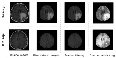
The preprocessing pipeline implemented in our framework comprises three distinct steps, as illustrated in Figure 2. Although skull stripping is conventionally performed after image enhancement, our framework demonstrated superior outcomes after performing skull stripping before image enhancement. This ordering addresses the specific characteristics of the data more effectively.
Figure 2. Preprocessing phase
The Eq. (1) defining the two-dimensional median filter is as follows:
$f(x, y)=\operatorname{median}_{(s, t) \in s_{x y}}\{g(s, t)\}\ and\ (p, t) \in P_{x y}$ (1)
$S_{x y}$ represent an $m \times n$ subimage of the input noisy image, $g$. It is centered at coordinates $(x, y) . f(x, y)$ represents the filter response at those coordinates. For a noisy image g centered at $(x, y)$ with an $m \times n$ subimage $S_{x y}$, the filter response at $(x, y)$ is defined by $f(x, y)$.
3.2 Tumor segmentation stage
This is the second and primary stage of our framework, which is ultimately responsible for producing the tumor segment. It involves several steps in which two modalities of brain MRI, T1-w and FLAIR, are processed. It includes edema segmentation from the flair image using the ICM algorithm, probability map generation from the T1-w image using the multi-scale FCM algorithm, automatic graph-cut segmentation of the tumor from T1-w, and post-processing enhancement of the segmented tumor using standard FCM.
3.2.1 Edema segmentation by ICM algorithm
The iterative conditional modes (ICM) algorithm was proposed by Besag [42] as an approximate solution to MAP estimation, and elegantly tackles the challenge of minimization by iteratively refining the labels, aiming to reduce the subsequent Eq. (2) at every pixel s:
$\hat{x}=\arg \min _{x_s \in L}\left\{\frac{\mathcal{Y}-\mu_s}{\sigma_s}+\frac{1}{2} \log \left(2 \pi \sigma_s^2\right)+\beta \mathcal{U}\left(x_s\right)\right\}$ (2)
$\mathcal{U}\left(x_s\right)$ is the number of pixels in the neighborhood that have color. In our case, is the intensity in the Flair image, and the equation between the brackets that combines Gibbs energy and negative log-likelihood is referred to as the total energy.
By redefining the conditional distribution of the MRF, as suggested by Besag [42], we can examine pairwise interactions.
$ \mathrm{P}\left(\mathrm{X}=x_s\right) \propto \exp \left(\sum_{s, r \in C} \beta_{s r} \delta\left(x_s, x_r\right)\right)$ (3)
where, $\delta\left(x_s, x_r\right)=\left\{\begin{array}{lc}1 & x_s=x_r \\ 0 & x_s \neq x_r\end{array}\right.$
In this first step, we intend to segment edema from Flair image by ICM algorithm, we have chose this modality because it provides ideal contrast between the tumor area and healthy tissue that facilitates differentiating the edema region. In addition, it has a higher contrast than the T1-w modality. In this stage, we defined three regions to be segmented (edema, background, and other tissues).
3.2.2 Multiscale FCM algorithm for probability maps generation
|
Algorithm 1: Multi-Scale Fuzzy C-Means |
|
Input: Original image T1-w Output: Probability maps: prob_map1, prob_map2, prob_map3 |
|
Step 1: Define Parameters Set num_scales = 3. Step 2: Initialize Probability Maps Initialize prob_map1 to zeros of the same size as T1-w. Initialize prob_map2 to zeros of the same size as T1-w. Initialize prob_map3 to zeros of the same size as T1-w. Step 3: Generate Multi-Scale Images For scale = 1 to num_scales Resize the image: scaled_image=Resize(T1-w,12scale−1\frac{1}{2^{\text{scale }-1}}2scale−11). Step 4: Perform FCM Clustering Step 5: Threshold Membership Values 5.1. Compute threshold 5.2. Generate binary map Step 6: Resize Binary Maps Resize the binary map to the original image size: binary_map = Resize (bw_map, size of T1-w). Step 7: Store Probability Maps If scale = 1: Set prob_map1 = Convert binary_map to double precision. Else if scale = 2: Set prob_map2 = Convert binary_map to double precision. Else if scale = 3: Set prob_map3 = Convert binary_map to double precision. Step 8: Output Probability Maps Return prob_map1, prob_map2, prob_map3. |
The multi-scale FCM processes the T1-w image at full, half, and quarter resolution to combine precise boundary detection from the fine scale with robust region identification from the coarse scale, making the algorithm more accurate and less sensitive to noise. The FCM is configured with 3 clusters, a fuzziness parameter of m=2.0, and a stopping criterion of ε=1e-5 at each level. The membership maps from all three scales are averaged to create a final probability map, from which the tumor seed is automatically generated by applying a threshold of 0.7. At each scale, the image is resized, and FCM clustering is applied to partition the image into segments. As illustrated in the pseudocode of the Algorithm 1. The output consists of a series of probability maps that indicate the likelihood of each pixel belonging to the tumor, edema, or background across different scales. These multiscale probability maps are subsequently utilized to assign background and foreground pixels for constructing graph cuts, as illustrated in the Algorithm 2.
|
Algorithm 2: Generate Foreground and Background Seeds |
|
Input: Segmentation //A matrix representing a segmentation map with different labels Outputs: Foreground seeds (fg_seeds) and Background seeds (bg_seeds) |
|
Step 1: Identify Unique Labels Check the number of unique labels in the segmentation map If the number of unique labels is less than two, report an error //Segmentation map must contain at least two different labels Step 2: Initialize Seed Arrays 2.1 Initialize fg_seeds = empty set 2.2 Initialize bg_seeds = empty set. Step 3: Process Each Label For each label in the segmentation map Create a mask isolating the current label Find all connected regions (components) within this mask Determine the size of each connected region Identify the largest connected region for the current label If processing the first label Add the largest region's coordinates to the background seed list Else Add the largest region's coordinates to the foreground seed list Step 4: Convert Collected Indices to Coordinates 4.1 Convert linear indices of fg_seeds to (x, y) coordinates 4.2 Convert linear indices of bg_seeds to (x, y) coordinates Step 5: Prepare the Seed Lists 5.1 Format fg_seeds as a list of (x, y) coordinates 5.2 Format bg_seeds as a list of (x, y) coordinates: Step 6: Return the Results Return fg_seeds and bg_seeds |
3.2.3 Tumor segmentation by Graph cuts method
A set of nodes (vertices) matching the image elements, which might represent pixels or regions in Euclidean space, is known as an undirected graph $G=(V, \mathrm{E}), V=\left\{v_1, \ldots, v_n\right\} . E$ is a collection of edges that joins certain sets of adjacent vertices. Each edge $\left(v_i, v_j\right) \in E$ has a corresponding weight $w\left(v_i, v_j\right)$ that measures a specific quantity dependent on the characteristics of the two nodes it connects [43].
Because this approach is based on neighborhood graphs, each pixel in the image is turned into a node in the graph, and edges from node connections of pixels that are neighbors. A graph’s relationship between a cut and a collection of edges as a result of G being divided into sets A and B, an image segmentation can be determined by Eq. (4).
${cut}(A, B)=\sum_{u \in A, v \in B} w(u, v)$ (4)
u and v correspond to the vertices of two distinct components.
Boykov and Funka-Lea [44] presented graph-cut segmentation. The key significant advance of object extraction in the graph cuts approach is the segmentation energy, which is expressed by binary variables whose values only indicate whether a pixel is present inside or outside the target area, Greig et al. [45] were the first to realize the strength of graph cut-based methods from combinatorial optimization for computer vision issues.
Considering $p$ as a set of pixels and $L$ as a set of labels, the goal is to find a labelling $f: P \rightarrow L$ that minimizes the energy:
$E(f)=R(f)+\lambda \cdot B(f)$ (5)
where,
$R(f)=\sum_{p \in P} R_p\left(f_p\right)$ (6)
and
$B(f)=\sum_{\{p, a \in N\}} B_{\{p, q\}} \delta\left(f_p, f_q\right)$ (7)
and
$\delta\left(f_p, f_q\right)=\left\{\begin{array}{lr}1 & { if }\ f_p \neq f_q \\ 0 & { Otherwise }\end{array}\right.$
The coefficients $\mathrm{R}_{\mathrm{p}}$ and $\mathrm{B}\{\mathrm{p}, \mathrm{q}\}$ are region and boundary terms that specify the penalties for assigning pixel p to "object" and "background," and a penalty for a discontinuity between p and q respectively. The cost function comprises region terms $R_p$, which penalize the assignment of a pixel $p$ to a label, and boundary terms $B\{p, q\}$, which penalize discontinuities between pixels $p$ and $q$.
In this second step, after generating the probability maps previously, the object and background seeds are then automatically assigned to build the graph, which is used for binary segmentation on ‘imgt1-w’ in order to extract the tumor region and produce its mask ‘maskTumor’. We chose the T1-w modality because it is useful for highlighting active tumors.
3.3 Post-processing Enhancements
The segmentation results were improved by applying standard fuzzy c-means. The FCM clustering algorithm was implemented by Professor Jim Bezdek in 1981 [46] based on the minimization of the following objective function:
$J_m=\sum_{i=1}^N \sum_{j=1}^C u_{i j}^m\left\|\mathrm{X}_{\mathrm{i}}-\mathrm{C}_{\mathrm{j}}\right\|^2$ (8)
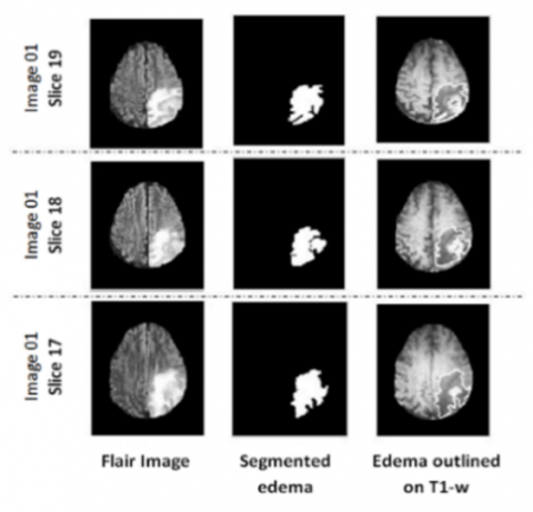
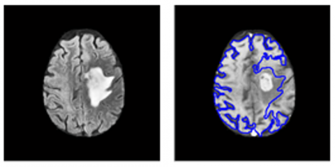
The segmentation outcomes derived from the proposed framework are defined as follows: First, the ICM algorithm is launched to perform segmentation of the Flair image into three regions: edema, background, and other tissues. The contour of the edema mask was then overlaid on the T1-w image to highlight the edema region. Figure 3 displays the results of applying ICM segmentation to three consecutive slices of the first patient’s case image. The outputs are the segmented edema region, edema mask “Maskedema” and the outlined T1-w image “imgT1-w”.
Figure 3. Edema segmentation by ICM algorithm: (a) Flair image; (b) Edema mask; (c) Edema mask outlined on T1-w image
A graph cuts based segmentation is then performed on “imgT1-w” to separate tumor region and produce its mask “maskTumor”. Segmentation is performed automatically without user intervention in selecting foreground and background pixels. Instead, it extracts these from the probability maps generated during the previous multiscale FCM segmentation step.
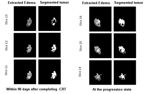
The outcomes of this investigation entail the documentation of two instances involving patients afflicted with glioblastoma. Two magnetic resonance examinations were acquired for every patient, specifically, the first within a period of 90 days subsequent to the conclusion of chemoradiotherapy and the second at the stage of disease progression, as illustrated in Figure 4 and Figure 5.
Figure 4. Graph cuts segmentation of tumor region for instance 1
Figure 5. Graph cuts segmentation of tumor region for instance 2
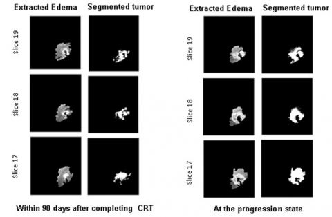
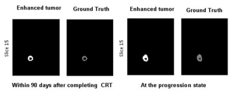
Finally, the tumor region “maskTumor” result obtained by graph cut segmentation is smoothed and enhanced by a second segmentation based on a standard FCM algorithm. The results of this inquiry involve recording two cases of patients suffering from glioblastoma, the first within a period of ninety days subsequent to the conclusion of chemoradiotherapy and the second at the stage of disease progression, as illustrated in Figures 6 and 7.
Figure 6. FCM-based enhancement of the tumor region for case 1
Figure 7. FCM-based enhancement of the tumor region for case 2
4.1 Visual evaluation
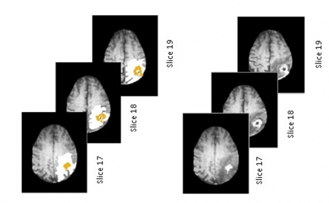
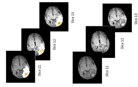
We conducted a qualitative assessment of the results produced by our segmentation framework through visual inspection and compared the segmented edema and tumor regions with ground truth annotations. As shown in Figures 8 and 9, the visual observations confirm that our method achieves highly accurate segmentations, with the segmented edema and tumor regions closely aligning with the ground truth.
Figure 8. Final segmentation results for image 01 at the progression state: segmented tumor and edema regions (left column), original T1-w image (right column)
Figure 9. Final segmentation results for image 01 at the progression state: segmented tumor and edema regions (left column), original T1-w image (right column)
The segmented images accurately captured the complex boundaries and structures of the tumors and edema, thereby demonstrating the effectiveness of the proposed method. The precise delineation of the tumor regions closely matched the ground truth, highlighting the robustness of our framework for accurate brain tumor segmentation from multimodal MR images.
4.2 Quantitative evaluation
The Dice index [47, 48] commonly referred to as the kappa ($\kappa$) coefficient, measures the intersection between a segmented region and a segmented ground-truth region, and takes the form of a scalar measure in the interval [0, 1]. It is calculated using this formula [48]:
$Dice=\frac{2 \times T P}{2 \times T P+F P+F N}$ (9)
where,
(1) TP: True positives are the number of pixels accurately identified as tumor
(2) FP: False Positives are the number of pixels that were mistakenly classified as tumor
(3) FN: False Negatives are the number of pixels that were incorrectly identified as background
Along with Dice index, we also evaluate tumor segmentation using the standard metrics of specificity (TNR), sensitivity (TPR) and Jaccard index:
$T N R=\frac{T N}{T N+F P}$ (10)
$T P R=\frac{T P}{T P+F N}$ (11)
$Jaccard =\frac{T P}{T P+F N+F P}$ (12)
4.2.1 Performance evaluation of ICM-based edema segmentation
Validation of the ICM algorithm for edema segmentation against expert manual annotations yielded an average Dice coefficient of 93%, confirming its high reliability.
4.2.2 Performance evaluation of tumor segmentation
We conducted a series of experiments on all 20 images, the results based on Dice and standard deviations (Std) are presented in Table![]() 1.
1.
Table 1. Average, Max. and Min. Dice index for the whole 20 cases, involving the proposed framework
|
Method |
Std |
Average Dice |
Max.Dice |
Min.Dice |
|
Our framework |
2.15 |
0.90 |
0.91 |
0.87 |
To demonstrate the contribution of the proposed framework, interactive-based segmentation of the tumor region from T1-w images was performed, and the results were compared with those obtained using the proposed framework. According to the results presented in Table 2, we can confirm that the proposed framework significantly improves tumor segmentation for the average value of the Dice coefficient compared with the interactive graph cut method, with an improvement of approximately 9%.
Table 2. Comparison of detection outcomes using the Dice index, obtained by the suggested framework and interactive graph cut
|
Method |
Average Dice |
Max.Dice |
Min.Dice |
|
Our framework |
0.90 |
0.91 |
0.87 |
|
Interactive graph cut |
0.81 |
0.83 |
0.75 |
The mean processing time of our fully-automated framework was 171.7 ± 7.2 seconds. By removing the variability and time demands of manual segmentation, our approach supports the incorporation of objective volumetric data into routine clinical workflows regarding radiation planning, therapy response assessment, and long-term surveillance.
To further test the efficiency and accuracy of the segmentation framework we developed, we calculated the Jaccard index, sensitivity, and specificity for all images. As shown in the Table 3, it gives almost the same values for these metrics for tumor segmentation from the images of all 20 patients, all images within 90 days after completing CRT, and at the progression state. These results demonstrate the robustness and efficiency of the proposed segmentation framework.
Table![]() 3. Jaccard index, sensitivity and specificity results of our framework overall 20 pre- and post-contrast agent images
3. Jaccard index, sensitivity and specificity results of our framework overall 20 pre- and post-contrast agent images
|
Within 90 days after completing CRT |
|||
|
Performance metrics |
Jaccard |
Sensitivity |
Specificity |
|
Brain tumor |
0.85 |
0.97 |
0.96 |
|
At the progression state |
|||
|
Performance metrics |
Jaccard |
Sensitivity |
Specificity |
|
Brain tumor |
0.85 |
0.98 |
0.96 |
Table 4 provides a comparative analysis of the performance between the proposed framework and several recent methods, evaluated in terms of Sensitivity, Specificity, PPV, NPV, and Accuracy. Our fully automated framework demonstrates superior results compared to contemporary methods. Specifically, it achieves values of 0.96 for Specificity, 0.98 for Sensitivity, 0.99 for NPV, 0.98 for PPV, and 0.99 for Accuracy.
Table 4. Comparison findings of the suggested workflow with those some of the most recent methods
|
Method |
Sensitivity |
Specificity |
PPV |
NPV |
Acc |
|
Our framework |
0.98 |
0.96 |
0.98 |
0.99 |
0.99 |
|
GRU/EHDMO [49] |
0.98 |
0.97 |
0.98 |
0.98 |
0.95 |
|
BrainMRNet [50] |
0.87 |
0.87 |
0.91 |
0.92 |
0.85 |
|
VGG19 [51] |
0.70 |
0.80 |
0.71 |
0.93 |
0.77 |
|
ASSO [52] |
0.59 |
0.65 |
0.82 |
0.90 |
0.65 |
|
CNN/POA [53] |
0.95 |
0.77 |
0.58 |
0.86 |
0.71 |
|
YOLOv2 [54] |
0.91 |
0.97 |
0.65 |
0.79 |
0.90 |
In one case (patient 10), where the intensity contrast is minimal between the edematous region and the surrounding healthy tissue, the algorithm's performance degrades. Such ambiguity affects the initial ICM-based segmentation of edema, thus impacting the accuracy of the subsequent tumor delineation, as shown in Figure 10.
Figure 10. Impact of ambiguous edema segmentation (case 10) on final tumor delineation
This study introduced a new graph-cut-based framework for fully automated brain tumor segmentation from multimodal MR images. Our method is unique in that it uses only T1-w and FLAIR modalities to segment both edema and tumors. Furthermore, the proposed segmentation framework is fully automatic, which is crucial for clinical applications, beginning as soon as both the Flair and T1-w images are read, which could help doctors monitor treatment progress. The most significant clinical implication of this work lies in its potential to integrate quantitative tumor burden assessment into standard radiological workflows. Currently, manual or semi-automated segmentation methods are too time-consuming for routine use, leading to a reliance on subjective, visual assessment of tumor size and evolution. Our fully-automated system, which requires no manual intervention, can generate an objective and reproducible segmentation in a matter of minutes. Perfect for monitoring therapies over time. The use of multimodal MRI data reinforces the robustness and versatility of the framework. While the proposed algorithm showed robust performance on the current dataset, a future validation on a larger, to further establish its generalizability. While this study demonstrates a robust fully-automated graph cut framework, future work will focus on enhancing the current pipeline. Immediate directions include: validation on larger datasets to assessing the generalization of our method across data from different hospitals and MRI scanner manufacturers. Streamlining the implementation to reduce processing time, facilitating real-time application in clinical settings, and adapting the framework to separately segment the enhancing tumor, necrotic core, and peritumoral edema, which is of high clinical relevance.
[1] Kamnitsas, K., Ledig, C., Newcombe, V.F.J., Simpson, J.P., Kane, A.D., Menon, D.K., Rueckert, D., Glocker, B. (2016). DeepMedic for brain tumor segmentation. In International Workshop on Brainlesion: Glioma, Multiple Sclerosis, Stroke and Traumatic Brain Injuries. Cham: Springer International Publishing, pp. 138-149. https://doi.org/10.1007/978-3-319-55524-9_14
[2] Zhuge, Y., Ning, H., Mathen, P., Cheng, J.Y., Krauze, A., Camphausen, K., Miller, R.W. (2017). Brain tumor segmentation using holistically nested neural networks in MRI images. Medical Physics, 44(10): 5234-5243. https://doi.org/10.1002/mp.12481
[3] Mohan, G., Subashini, M.M. (2018). MRI-based medical image analysis: Survey on brain tumor grade classification. Biomedical Signal Processing and Control, 39: 139-161. https://doi.org/10.1016/j.bspc.2017.07.007
[4] Gooya, A., Biros, G., Davatzikos, C. (2012). GLISTR: Glioma image segmentation and registration. IEEE Transactions on Medical Imaging, 31(10): 1941-1954. https://doi.org/10.1109/TMI.2012.2210558
[5] Wang, M.Q., Yang, J., Chen, Y.L., Wang, H. (2017). The multimodal brain tumor image segmentation based on convolutional neural networks. In 2017 2nd IEEE International Conference on Computational Intelligence and Applications (ICCIA), Beijing, China, pp. 336-339. https://doi.org/10.1109/CIAPP.2017.8167234
[6] Wang, Y., Ye, X. (2023). U-Net multi-modality glioma MRIs segmentation combined with attention. In 2023 International Conference on Intelligent Supercomputing and BioPharma (ISBP), Zhuhai, China, pp. 82-85. https://doi.org/10.1109/ISBP57705.2023.10061312
[7] Sehgal, A., Goel, S., Mangipudi, P., Mehra, A., Tyagi, D. (2016). Automatic brain tumor segmentation and extraction in MR images. In 2016 Conference on Advances in Signal Processing (CASP), Pune, India, pp. 104-107. https://doi.org/10.1109/CASP.2016.7746146
[8] Rasool, N., Bhat, J.I. (2023). Glioma brain tumor segmentation using deep learning: A review. In 2023 10th International Conference on Computing for Sustainable Global Development (INDIACom), New Delhi, India, pp. 484-489.
[9] Yang, H., Zhou, T., Zhou, Y., Zhang, Y., Fu, H. (2023). Flexible fusion network for multi-modal brain tumor segmentation. IEEE Journal of Biomedical and Health Informatics, 27(7): 3349-3359. https://doi.org/10.1109/JBHI.2023.3271808
[10] Iyer, G., Chanussot, J., Bertozzi, A.L. (2017). A graph-based approach for feature extraction and segmentation of multimodal images. In 2017 IEEE International Conference on Image Processing (ICIP), Beijing, China, pp. 3320-3324. https://doi.org/10.1109/ICIP.2017.8296897
[11] Iyer, G., Chanussot, J., Bertozzi, A.L. (2020). A graph-based approach for data fusion and segmentation of multimodal images. IEEE Transactions on Geoscience and Remote Sensing, 59(5): 4419-4429. https://doi.org/10.1109/TGRS.2020.2971395
[12] Mo, S., Chen, J., Zhang, W., Duan, J., Sun, Q., Ding, C., Tao, D. (2021). Mutual information-based graph co-attention networks for multimodal prior-guided magnetic resonance imaging segmentation. IEEE Transactions on Circuits and Systems for Video Technology, 32(5): 2512-2526. https://doi.org/10.1109/TCSVT.2021.3112551
[13] Vamsidhar, D., Desai, P., Joshi, S., Deshmukh, P.V., More, A.S. (2025). Optimized graph-based segmentation for brain tumor detection. Ingénierie des Systèmes d’Information, 30(3): 771-778. https://doi.org/10.18280/isi.300321
[14] Ali, A.M., Farag, A.A. (2007). Graph cut-based segmentation of multimodal images. In 2007 IEEE International Symposium on Signal Processing and Information Technology, Giza, Egypt, pp. 1036-1041. https://doi.org/10.1109/ISSPIT.2007.4458212
[15] Lecoeur, J., Ferré, J.-C., Collins, D.L., Morrisey, S.P., Barillot, C. (2009). Multi-channel MRI segmentation with graph cuts using spectral gradient and multidimensional Gaussian mixture model. In Medical Imaging 2009: Image Processing, 7259: 1268-1278. https://doi.org/10.1117/12.811108
[16] Beaumont, J., Commowick, O., Barillot, C. (2016). Multiple sclerosis lesion segmentation using an automated multimodal graph cut. In Proceedings of the 1st MICCAI Challenge on Multiple Sclerosis Lesions Segmentation Challenge Using a Data Management and Processing Infrastructure--MICCAI-MSSEG, Athens, Greece, pp. 1-8.
[17] Joshi, A., Sharma, K.K. (2022). Multi-modal lesion segmentation using deep convolution graph-based network. In 2022 IEEE Delhi Section Conference (DELCON), New Delhi, India, pp. 1-6. https://doi.org/10.1109/DELCON54057.2022.9752917
[18] Han, D., Bayouth, J., Song, Q., Taurani, A., Sonka, M., Buatti, J., Wu, X. (2011). Globally optimal tumor segmentation in PET-CT images: A graph-based co-segmentation method. In Biennial International Conference on Information Processing in Medical Imaging. Berlin, Heidelberg: Springer Berlin Heidelberg, pp. 245-256. https://doi.org/10.1007/978-3-642-22092-0_21
[19] Wang, X., Li, Y., Liu, H., Ding, X., Wang, Z., Liu, G. (2014). Lung tumor delineation based on novel tumor-background likelihood models in PET-CT images. IEEE Transactions on Nuclear Science, 61(1): 218-224. https://doi.org/10.1109/TNS.2013.2295975
[20] Ju, W., Xiang, D., Zhang, B., Wang, L., Kopriva, I., Chen, X. (2015). Random walk and graph cut for co-segmentation of lung tumor on PET-CT images. IEEE Transactions on Image Processing, 24(12): 5854-5867. https://doi.org/10.1109/TIP.2015.2488902
[21] Bagci, U., Udupa, J.K., Yao, J., Mollura, D.J. (2012). Co-segmentation of functional and anatomical images. In International Conference on Medical Image Computing and Computer-Assisted Intervention. Berlin, Heidelberg: Springer Berlin Heidelberg, pp. 459-467. https://doi.org/10.1007/978-3-642-33454-2_57
[22] Bauer, S., Fejes, T., Slotboom, J., Wiest, R., Nolte, L.P., Reyes, M. (2012). Segmentation of brain tumor images based on integrated hierarchical classification and regularization. In MICCAI BraTS Workshop. Nice: MICCAI Society.
[23] Zikic, D., Glocker, B., Konukoglu, E., Criminisi, A., Shotton, J. (2012). Context-sensitive classification forests for segmentation of brain tumor tissues. Proceedings of MICCAI BraTS, pp. 22-30.
[24] Tustison, N.J., Avants, B.B., Cook, P.A., Zheng, Y., Egan, A., Yushkevich, P.A., Gee, J.C. (2015). Optimal symmetric multimodal templates and concatenated random forests for supervised brain tumor segmentation (simplified) with ANTsR. Neuroinformatics, 13(2): 209-225. https://doi.org/10.1007/s12021-014-9245-2
[25] Reza, S., Iftekharuddin, K. (2013). Multi-class abnormal brain tissue segmentation using texture. Multimodal Brain Tumor Segmentation, 38: 38-42.
[26] Ghaffari, M., Sowmya, A., Oliver, R. (2019). Automated brain tumor segmentation using multimodal brain scans: A survey based on models submitted to the BraTS 2012-2018 challenges. IEEE Reviews in Biomedical Engineering, 13: 156-168. https://doi.org/10.1109/RBME.2019.2946868
[27] Kofler, F., Berger, C., Waldmannstetter, D., Lipkova, J., Ezhov, I., Tetteh, G., Zimmer, C., Menze, B.H., Subbanna, N.K. (2020). BraTS toolkit: Translating BraTS brain tumor segmentation algorithms into clinical and scientific practice. Frontiers in Neuroscience, 14: 125. https://doi.org/10.1109/RBME.2019.2946868
[28] Urban, G., Bendszus, M., Hamprecht, F., Kleesiek, J. (2014). Multi-modal brain tumor segmentation using deep convolutional neural networks. MICCAI BraTS (brain tumor segmentation) Challenge. Proceedings, Winning Contributions, pp. 31-35.
[29] Zikic, D., Ioannou, Y., Brown, M., Criminisi, A. (2014). Segmentation of brain tumor tissues with convolutional neural networks. Proceedings of MICCAI-BRATS, 36: 36-39.
[30] Havaei, M., Dutil, F., Pal, C., Larochelle, H., Jodoin, P.M. (2015). A convolutional neural network approach to brain tumor segmentation. In International Workshop on Brainlesion: Glioma, Multiple sclerosis, Stroke and Traumatic Brain Injuries. Cham: Springer International Publishing, pp. 195-208. https://doi.org/10.1007/978-3-319-30858-6_17
[31] Dvořák, P., Menze, B. (2015). Local structure prediction with convolutional neural networks for multimodal brain tumor segmentation. In International MICCAI Workshop on Medical Computer Vision, pp. 59-71. https://doi.org/10.1007/978-3-319-42016-5_6
[32] Kamnitsas, K., Ledig, C., Newcombe, V.F.J., Simpson, J.P., Kane, A.D., Menon, D.K., Rueckert, D., Glocker, B. (2017). Efficient multi-scale 3D CNN with fully connected CRF for accurate brain lesion segmentation. Medical Image Analysis, 36: 61-78. https://doi.org/10.1016/j.media.2016.10.004
[33] Wang, G., Li, W., Ourselin, S., Vercauteren, T. (2017). Automatic brain tumor segmentation using cascaded anisotropic convolutional neural networks. In International MICCAI Brainlesion Workshop, Quebec City, Canada, pp. 178-190. https://doi.org/10.1007/978-3-319-75238-9_16
[34] Yang, T., Ou, Y., Huang, T. (2017). Automatic segmentation of brain tumor from MR images using SegNet: Selection of training data sets. Proceedings of the 6th MICCAI BraTS Challenge, pp. 309-312.
[35] Myronenko, A. (2018). 3D MRI brain tumor segmentation using autoencoder regularization. In International MICCAI Brainlesion Workshop, Granada, Spain, pp. 311-320. https://doi.org/10.1007/978-3-030-11726-9_28
[36] Jiang, Y., Zhang, Y., Lin, X., Dong, J., Cheng, T., Liang, J. (2022). SwinBTS: A method for 3D multimodal brain tumor segmentation using Swin Transformer. Brain Sciences, 12(6): 797. https://doi.org/10.3390/brainsci12060797
[37] Liu, H., Wei, D., Lu, D., Sun, J., Wang, L., Zheng, Y. (2023). M3AE: Multimodal representation learning for brain tumor segmentation with missing modalities. In Proceedings of the AAAI Conference on Artificial Intelligence, 37(2): 1657-1665. https://doi.org/10.1609/aaai.v37i2.25253
[38] Clark, K., Vendt, B., Smith, K., Freymann, J., Kirby, J., Koppel, P., Moore, S., Phillips, S., Maffitt, D., Pringle, M., Tarbox, L., Prior, F. (2013). The Cancer Imaging Archive (TCIA): Maintaining and operating a public information repository. Journal of Digital Imaging, 26(6): 1045-1057. https://doi.org/10.1007/s10278-013-9622-7
[39] Schmainda, K., Prah, M. (2018). Data from brain-tumor-progression. Cancer Imaging Archive, 21.
[40] Kavitha, S., Inbarani, H. (2021). COVID-19 and MRI image denoising using wavelet transform and basic filtering. In 2021 5th International Conference on Intelligent Computing and Control Systems (ICICCS), Madurai, India, pp. 792-799. https://doi.org/10.1109/ICICCS51141.2021.9432307
[41] Kaur, H., Sohi, N. (2017). A study for applications of histogram in image enhancement. International Journal of Engineering Science, 6(6): 59-63. https://doi.org/10.9790/1813-0606015963
[42] Besag, J. (1986). On the statistical analysis of dirty pictures. Journal of the Royal Statistical Society. Series B (Methodological), 48(3): 259-302. https://doi.org/10.1111/j.2517-6161.1986.tb01412.x
[43] Peng, B., Zhang, L., Zhang, D., Yang, J. (2011). Image segmentation by iterated region merging with localized graph cuts. Pattern Recognition, 44(10-11): 2527-2538. https://doi.org/10.1016/j.patcog.2011.03.024
[44] Boykov, Y., Funka-Lea, G. (2006). Graph cuts and efficient ND image segmentation. International Journal of Computer Vision, 70(2): 109-131. https://doi.org/10.1007/s11263-006-7934-5
[45] Greig, D.M., Porteous, B.T., Seheult, A.H. (1989). Exact maximum a posteriori estimation for binary images. Journal of the Royal Statistical Society. Series B (Methodological), 51(2): 271-279. https://doi.org/10.1111/j.2517-6161.1989.tb01764.x
[46] Bezdek, J. (1981). Pattern Recognition with Fuzzy Objective Function Algorithms. Springer Science & Business Media. https://doi.org/10.1007/978-1-4757-0450-1
[47] Sørensen, T.J. (1948). A method of establishing groups of equal amplitude in plant sociology based on similarity of species content and its application to analyses of the vegetation on Danish commons. I kommission hos E. Munksgaard.
[48] Dice, L.R. (1945). Measures of the amount of ecologic association between species. Ecology, 26(3): 297-302. https://doi.org/10.2307/1932409
[49] Yang, Y., Chaoluomeng, Razmjooy, N. (2024). Early detection of brain tumors: Harnessing the power of GRU networks and hybrid dwarf mongoose optimization algorithm. Biomedical Signal Processing and Control, 91: 106093. https://doi.org/10.1016/j.bspc.2024.106093
[50] Toğaçar, M., Ergen, B., Cömert, Z. (2020). BrainMRNet: Brain tumor detection using magnetic resonance images with a novel convolutional neural network model. Medical Hypotheses, 134: 109531. https://doi.org/10.1016/j.mehy.2019.109531
[51] Rajinikanth, V., Raj, A.N.J., Thanaraj, K.P., Naik, G.R. (2020). A customized VGG19 network with concatenation of deep and handcrafted features for brain tumor detection. Applied Sciences, 10(10): 3429. https://doi.org/10.3390/app10103429
[52] Deb, D., Roy, S. (2021). Brain tumor detection based on hybrid deep neural network in MRI by adaptive squirrel search optimization. Multimedia Tools and Applications, 80(2): 2621-2645. https://doi.org/10.1007/s11042-020-09810-9
[53] Tian, Q., Wu, Y., Ren, X., Razmjooy, N. (2021). A new optimized sequential method for lung tumor diagnosis based on deep learning and converged search and rescue algorithm. Biomedical Signal Processing and Control, 68: 102761. https://doi.org/10.1016/j.bspc.2021.102761
[54] Sharif, M.I., Li, J.P., Amin, J., Sharif, A. (2021). An improved framework for brain tumor analysis using MRI based on YOLOv2 and convolutional neural network. Complex and Intelligent Systems, 7(4): 2023-2036. https://doi.org/10.1007/s40747-021-00310-3