Sonia Benabid*![]() | Sofiane Maza
| Sofiane Maza![]() | Abdelouahab Attia
| Abdelouahab Attia![]() | Nour Elhouda Chalabi
| Nour Elhouda Chalabi![]() | Youssef Chahir
| Youssef Chahir![]()
© 2025 The authors. This article is published by IIETA and is licensed under the CC BY 4.0 license (http://creativecommons.org/licenses/by/4.0/).
OPEN ACCESS
Finger Knuckle Print (FKP) is a promising biometric modality for personal recognition; however, existing methods still suffer from sensitivity to illumination variations and limited interpretability of deep learning models. To address these limitations, this paper proposes a novel explainable deep neural network (xDNN)-based Principal Component Analysis Network (PCANet) framework that combines robust feature extraction with transparent decision-making for FKP recognition. The Self-Quotient Image (SQI) method is applied to decompose FKP images into illumination-invariant reflectance components, mitigating lighting variations. Also, a two-stage of PCANet that extracts discriminative features from these components, leveraging its efficiency and hierarchical representation capability. To improve the trustworthiness of biometric decision-making, the framework incorporates the explainable Deep Neural Network (xDNN) approach for user identification. To enhance trust and transparency in biometric decision-making, the framework integrates an explainable Deep Neural Network (xDNN) that generates prototype-based reasoning and feature relevance visualizations, providing insight into the decision process and interpretability of classification outcomes. The proposed system is rigorously evaluated on the PolyU FKP database using all four finger types (Left Index Finger, Left Middle Finger, Right Index Finger, and Right Middle Finger) in a unimodal configuration. Key hyperparameters of SQI and PCANet are optimized through ablation studies to boost performance. The system achieves 91–96% identification accuracy, surpassing state-of-the-art methods, while offering interpretability lacking in previous approaches—making it well-suited for security-critical applications.
biometric system, FKP recognition, SQI algorithm, PCANet, xDNN
Recently a biometric system is considered as an alternative authentication and identification system to traditional methods (ID card, passwords, PIN codes). Biometrics recognition system facilitates the recognition process of a person by using her unique physiological and behavioral characteristics [1, 2]. As a result, many different biometric traits have been investigated widely, such as Fingerprint, Iris, Ear, Finger knuckle print, Palmprint, Face etc. [3-5]. However, Finger Knuckle Print (FKP) [6], included in the hand based biometric traits that have been intensively studied in order to improve the consistent authentication system with higher accuracy [7, 8]. FKP has distinctive anatomical structures that can be recorded with low cost and small size imaging devices without using an extra hardware [6, 8].
Generally, FKP recognition system splits into two tasks: (i) FKP identification: in this case, the focus of FKP identification system is to put a given FKP test into one of several predefined sets in a database, whereas (ii) FKP verification process is to determine if two FKP images belong to the same person. In addition, the FKP verification task is more difficult than FKP identification because in matching stage is required to give a global threshold in order to make a decision. Till now, the FKP recognition system has been attracting considerable attention of researchers over recent years. Several contributions were developed. Such as, Woodard and Flynn [9] and Woodard and Flynn [10] are among the first researchers who introduce the use of finger knuckle surface in biometric systems. Ferrer et al. [11] have proposed a framework based on a ridge feature-based algorithm. This method started with extracts ridge features from FKP images and evaluates their similarity using Hidden Markov Model (HMM) or Support Vector Machine (SVM). Zeinali et al. [12] have proposed a system for recognition FKP that the Directional Filter Bank (DFB) has been used for feature extraction. Then LDA is used to reduce the dimensionality of the large feature vector. Chaa et al. [13] in step of feature extraction, two types of Histogram of Oriented Gradients (HOG)-based features extracted from the reflectance and illumination components of FKP images for personal identification. The Adaptive Single Scale Retinex (ASSR) algorithm is employed to decompose each FKP image into its illumination and reflectance components. Then, the HOG descriptor applied on both extracted images (real and imaginary). These feature vectors concatenated together. Serial feature fusion is employed to construct a comprehensive feature vector for each user, enabling the extraction of distinctive characteristics within a higher-dimensional feature space. Finally, classification is performed using the cosine similarity distance measure. Zhang et al. [14] presented a new computation framework that focused on mounting new efficient feature extraction method for FKP recognition. The authors analyzed three commonly used local features, the local orientation, the local phase, and the phase congruency systematically. However, they presented a method for computing all features efficiently using the phase congruency. Li et al. [15] have introduced a feature extraction method employing steerable filters that can extract local orientation from FKP images. Recently deep networks methods learning called deep learning has emerge. This new area has been attracting considerable attention of researchers. Therefore, Qian et al. [4] have proposed a novel biometric image feature representation technique, known as exploring deep gradient information (DGI). Meraoumia et al. [16] have introduced a novel framework for a biometric identification system using PCANet deep learning and multispectral Palmprint. However, the basic idea of deep learning is to discover multiple levels of representation of the discriminant characteristics of biometric modalities effectively and efficiently. Chlaoua et al. [17] pioneered a computationally efficient FKP recognition system by combining PCANet feature extraction with SVM classification on PolyU datasets. Their key innovation involved optimizing PCANet's filter banks specifically for knuckle patterns, followed by kernel-based SVM refinement.
Recent studies highlight the limitations of "black-box" deep learning models in sensitive domains like biometrics, where decision transparency is crucial [18-20]. For that reason, in this paper, we propose a new recognition biometric system using the FKP traits based on the xDNN classifier receiving as inputs vector results from feature extraction by PCANet deep learning method and preprocessing by the Self-Quotient Image (SQI) method to decompose FKP images into illumination-invariant reflectance components, mitigating lighting variations. In this work, we develop unimodal recognition biometrics systems. We search the best value for parameters of both PCANet and SQI algorithm that get the best performances value. These parameters allow us to enhance the quality of xDNN feature extraction, which increase the detection and identification accuracy.
Our main contribution given in this paper are:
•Using an Explainable Deep Neural Network xDNN Classifier, a supervised deep learning framework designed for high accuracy pattern recognition while maintaining interpretability of decisions.
•Feature extraction combining SQI algorithm (Self-Quotient Image) method to decompose FKP images into illumination-invariant reflectance components, mitigating lighting variations and Initial extraction using PCANet Deep Learning technique.
•A comparison study of several experimental results is illustrated for different FKP modalities and recent well-known approaches.
The rest of this paper is organized as follows: In section 2, the xDNN classifier mechanism is presented then in section 3, the, proposed methodology FKP recognition system is described. We present all process steps of the system in detail with their techniques and functions. Section 4 presents the experimental results that illustrate the dataset used, performances metrics, parameters study of SQI algorithm and PCANet descriptor to select the best values. A comparison study is elaborated to compare between the proposed system and other well-known previous work. Finally, the conclusion and future work are given in the last section.
This work centers on explainable Deep Neural Networks (xDNN), a framework designed to unite high-accuracy learning with human-interpretable decision processes. While conventional deep models excel in performance, their opacity hinders trust in sensitive applications. xDNN overcomes this by embedding transparency directly into its architecture, enabling users to trace and validate its reasoning. Critically, mastering xDNN’s internal dynamics: such as [specific mechanisms, e.g., 'adaptive feature weighting' or 'dynamic rule generation'] is vital not only to deploy it effectively but also to justify its outputs in real-world scenarios.
2.1 The xDNN classifier: Core architecture and design principles
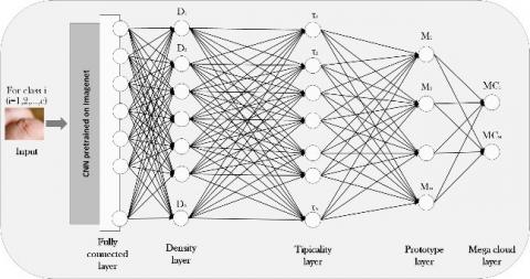
The proposed Explainable Deep Neural Network (xDNN) implements a dynamic feedforward structure capable of autonomous architectural evolution through continuous model adaptation. Unlike conventional static neural networks, this framework progressively restructures its layered organization in response to emerging pattern recognition demands. As illustrated in Figure 1, the system's five specialized processing layers operate in concert to enable:
•Adaptive feature space reconstruction.
•On-demand neural module generation.
•Transparent decision pathway formation.
Figure 1. xDNN Classifier’s architecture
These five functionally specialized layers that collectively execute the pattern recognition tasks. For complete understanding, we subsequently: define each layer's computational role, describe its structural configuration, and explain its sub-processes within the complete classification framework.
2.1.1 Feature descriptor layer: High-level feature extraction
The first critical step in the xDNN pipeline is feature extraction, where raw image data is transformed into meaningful numerical representations. While traditional methods like PCA or handcrafted filters (e.g., Gabor) have been widely used, they often struggle with capturing complex, non-linear patterns. A pre-trained deep convolutional neural network (DCNN) [21] known for its ability to extract highly discriminative features. From the recommendation of Ioffe and Szegedy [22] to incorporate normalization for deep feature stabilization and improve convergence.
The standardization and normalization of the extracted features become a crucial in such process and followed the Eqs. (1) and (2) respectively:
$\hat{x}_{i, j}=\frac{x_{i, j}-\mu\left(x_{i, j}\right)}{\sigma\left(x_{i, j}\right)}$ (1)
$\hat{x}_{i, j}=\frac{\hat{x}_{i, j}-\min _i\left(\hat{x}_{i, j}\right)}{\max _j\left(\hat{x}_{i, j}\right)-\min _i\left(\hat{x}_{i, j}\right)}$ (2)
$\hat{x}$ represents a standardized features vector x (the values provided by the FCL) of the image I and $\overline{\mathrm{x}}$ is the normalized value of the features vector, i is for the image’s ID, j is the current feature of x, I is the current image and N is the number of the images. The later step ensures all features contribute equally during classification.
xDNN initializes its meta-parameter (learning parameters) dynamically, eliminating the need for manual tuning. When the first data sample arrives, the system automatically configures different parameters as it is mentioned in Eq. (3):
$\begin{gathered}P \leftarrow 1 ; \mu \leftarrow x_i ; \\ C_1 \leftarrow x_1 ; p_1 \leftarrow x_1 ; \text { Support }_1 \leftarrow 1 ; r_1 \leftarrow r^* ; \hat{I}_1 \leftarrow I_1\end{gathered}$ (3)
P for prototype, C for class, Support for the equivalent support (number of members) belonging to the identified Model, r for the equivalent radius of the area of influence of the Class $C_i, \mu$ is the global mean of the class, I is the current image and $\hat{\mathrm{I}}$ is the identified prototype.
The dynamic radius calculation method follows the data-derived approach proposed by Angelov and Gu [23] for autonomous system parameterization.
Following the methodology outlined in the study [24], we obtain the critical threshold $r^*=\sqrt{2-2 \cos \left(30^{\circ}\right)}$.
The Rational r*metric represents an analytically derived boundary rather than an empirically tuned parameter. It is delineated when the angle subtended by two vectors is less than 30° and they are oriented in the same direction denoted by d. Building upon this foundation, we examine two feature vectors that exhibit an angle of less than 30° between them, categorizing them as “Similar”. The determination of the direction d is achieved through the application of Eq. (4).
$d\left(x_i, p_i\right)=\left\|\frac{x_i}{\left\|x_i\right\|}-\frac{p_i}{\left\|p_i\right\|}\right\|$ (4)
2.1.2 Density layer
This layer plays a crucial role in establishing the shared proximity among the images within the data space from the layer before it. The data distribution follows a Cauchy pattern when employing the Euclidean distance, as demonstrated in the study [24] Unlike Gaussian kernels, the Cauchy distribution better handles outliers, making it suitable for real-world biometric data [25]. The data density D is determined through the formula in Eq. (5) or Eq. (6).
$D\left(x_i\right)=\frac{1}{1+\frac{\left\|x_i-\mu N\right\|^2}{\sigma_N^2}}$ (5)
$D\left(x_i\right)=\frac{1}{1+\left\|x_i \mu_i\right\|^2+\sum_i-\left\|\mu_i\right\|^2}$ (6)
The scalar coefficient $\Sigma_i$ can be updated as in Eq. (7), where $\mu_i$ is involved.
$\begin{gathered}\mu_i \leftarrow \frac{i-1}{i} \mu_{i-1}+\frac{1}{i} x_i \\ \sum_i=\frac{1}{1-i} \sum_{i-1}+\frac{1}{i}\left\|x_i\right\|^2 \sum_1^2=\left\|x_1\right\|^2\end{gathered}$ (7)
Higher density values indicate stronger cluster cohesion. Consequently, the solid mutual influence between the images in the space of data due to their common adjacency.
2.1.3 Typicality layer
Typicality $\tau$ quantifies how well a sample fits within its class distribution based on the probability distribution function, which is determined by utilizing the Eq. (8). It is a probabilistic confidence scoring.
$\tau\left(x_i\right)=\frac{\sum_i^c \text { Support }_i D\left(x_i\right)}{\sum_i^c \text { Support }_i \int_{-\infty}^{+\infty} D\left(x_i\right) d x}$ (8)
The typicality is between 0 and 1, peaks near prototype vectors, declining towards outliers. A high $\tau$ means high confidence in classification. The value of $\tau$ remains consistently below the value 1.
2.1.4 Prototypes or Models Layer
xDNN constructs human-readable IF-THEN rules (Transparent Rule-Based Learning) for each class. The IF-THEN rule generation implements the transparent fuzzy rule extraction method from the research [26]. The dynamic model expansion criteria refine the concept of "novelty detection" described in Markou and Singh [27]. The xDNN architecture implements a novel paradigm for explainable artificial intelligence through its innovative Models Layer. This component establishes a dynamic, self-organizing framework that learns data distributions directly from visual inputs without relying on predetermined statistical assumptions. The system's modular design philosophy enables independent operation of each classification model, permitting seamless integration of new recognition categories while preserving existing knowledge structures, a critical advantage for scalable biometric applications. The Models Layer constitutes the foundational interpretable framework within an xDNN biometric system. This component uniquely operates without requiring prior assumptions about data distributions, instead deriving its understanding directly from visual patterns in the input images. The architecture's modular independence represents a significant innovation. New models can be incorporated without affecting existing ones, which enables seamless system expansion while maintaining operational stability. During the training phase, xDNN performs class-specific processing to develop distinct model sets that capture the essential density characteristics identified in earlier stages. These models generate human-readable decision rules following the logical structure:
IF (input ∼ prototype K₁) THEN classify as Class C
The symbol ~ denotes similarity and the degree of membership. One rule can be generated for the same model, however, the same class’s rules are connected by the logical disjunction OR as followed:
$\begin {gathered} IF \left(input \, \sim prototype \, K_1\right) OR \ldots OR \left(input \sim prototype \, K_m\right) THEN \, classify \, as \, Class \, C\end {gathered}$
Each model establishes a Data Cloud [18], a dynamic region encompassing similar feature vectors. Unlike traditional approaches using statistical means, these clouds center around actual representative samples. The system employs an intelligent assignment mechanism that continuously evaluates new inputs against existing prototypes using minimum distance criteria:
$j^*=\underset{j=1,2 \ldots p}{\operatorname{argmin}}\left(\left\|x_i-p_j\right\|^2\right)$ (9)
The system dynamically generates new recognition clusters when either of these density conditions is met:
$\begin{aligned}&\begin{aligned}& \operatorname{IF}\left(D\left(x_i\right) \geq \max _{j=1,2, \ldots, p} D\left(p_j\right)\right) \\& \operatorname{OR}\left(D\left(x_i\right) \leq \min _{j=1,2, \ldots, p} D\left(p_j\right)\right)
\end{aligned}\\&\operatorname{THEN}(\text { add a new data cloud }(P \leftarrow P+1))\end{aligned}$ (10)
Cluster initialization
$\begin{aligned} & P \leftarrow P+1 ; C_P \leftarrow x_i ; p_P \leftarrow I_i ; \\ & \text { Support }_P \leftarrow 1 ; r_P \leftarrow r_o ; \hat{I}_P \leftarrow I_i\end{aligned}$ (11)
For existing clusters, the system performs incremental updates:
$\begin{gathered}C_{j^*} \leftarrow C_{j^*}+1 ; p_{j^*} \leftarrow \frac{\text { Support }_{j^*}}{\text { Support }_{j^*}+1} p_{j^*} \\ +\frac{\text { Support }_{j^*}}{\text { Support }_{j^*}+1} x_i ; \text { Support }_{j^*} \\ \leftarrow \text { Support }_{j^*}+1 ; r_{j^*}^2 \leftarrow \frac{r_{j^*}^2+\left(1-\left\|p_{j^*}\right\|^2\right)}{2}\end{gathered}$ (12)
The layer's adaptive nature allows for organic system growth while maintaining classification accuracy, making it particularly suitable for evolving biometric applications where new classes may need periodic incorporation.
2.1.5 Mega cloud layer
The cloud fusion algorithm extends the traditional hierarchical aggregation approach by introducing angular similarity constraints, which strengthen the clustering process. In the MegaClouds layer, clouds produced in the previous stage are combined whenever neighboring prototypes share the same class label. This merging process forms larger clusters, referred to as Mega Clouds (MCs), thereby improving the interpretability of the system:
$\begin{gathered}R_c: \operatorname{IF}\left(\bar{v}_{\imath} \sim M C_1\right) \text { OR }\left(\bar{v}_{\imath} \sim M C_2\right) \text { OR } \ldots \text { OR }\left(\bar{v}_{\imath}\right. \\ \left.\sim M C_m\right) \text { THEN Class }\end{gathered}$
where, MCi denotes the Mega Clouds, which represent the regions formed by merging smaller clouds belonging to the same class, and MC is the total number of identified Mega Clouds. This step aims to reduce rule complexity while maintaining high transparency for end-users, ensuring that classification decisions remain both accurate and interpretable.
|
Algorithm 1. xDNN classifier’s algorithm [18] |
|
xDNN Learning Level Step A: Initialization 1: Read the first feature vector sample $x_i$ representing the image $I_i$ of the class c 2: initiate $\begin{gathered}i \leftarrow 1 ; n \leftarrow 1 ; P_1 \leftarrow 1 ; p_1 \leftarrow x_i ; \mu \leftarrow x_1 ; \text { Support } \leftarrow 1 ; r_1 \leftarrow r_0 ; \hat{I}_1 \leftarrow I_1 ;\end{gathered}$ Step B: Execution 3: FOR i = 2, ... 4: Read $x_i$; 5: Compute $D\left(x_i\right)$ and $D\left(p_j\right) \quad(j=1,2, \ldots, P)$ according to Eq. (9) 6: IF Eq. (12) holds 7: Generate rule according to Eq. (13); 8: ELSE 9: Search for $p_i$ according to Eq. (11); 10: Update rule according to Eq. (14); 11: END 12: END |
The proposed research relies on an explainable deep neural network image-based framework and explore it in different data base of FKP trait which is principally characterized by explainability Further, it presents human- interpretable layers. Consciously, the architecture of the xDNN classifier is entirely transparent and evident to explain to human user.
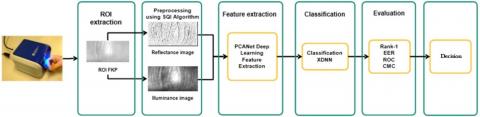
As shown in Figure 2 the proposed biometric system is mainly composed of 4 main steps:
Step 1: Image acquisition and normalization: The input Finger-Knuckle Print (FKP) images are captured and normalized to ensure consistency in scale and orientation.
Step 2: Illumination-invariant preprocessing: The SQI algorithm is applied to decompose FKP images into reflectance components, reducing sensitivity to lighting variations and enhancing robustness.
Step 3: Hierarchical feature extraction: A PCANet-based deep learning framework performs initial feature extraction, leveraging its efficiency in capturing discriminative patterns through principal component analysis.
Step 4: Explainable classification (xDNN): The extracted features are processed through an explainable Deep Neural Network (xDNN), which includes:
Feature layer: Encodes high-level representations.
Density layer: Models data distribution.
Typicality layer: Assesses similarity to learned prototypes.
Mega cloud layer: Aggregates global patterns for decision support.
Figure 2. The proposed biometric system’s architecture
3.1 ROI extraction
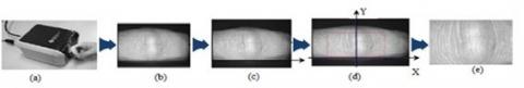
The extraction of the ROI from FKP images involves multiple steps [8]:
(i) First, a Gaussian smoothing filter is applied to the original FKP image, followed by downsampling the smoothed result to a resolution of 150 dpi. (ii) Next, the X-axis of the coordinate system is determined by referencing the lower boundary of the finger, which is detected using the Canny edge detection algorithm. (iii) To define the Y-axis, a sub-region of the image—cropped based on the X-axis—is processed with the Canny edge detector. Then, a convex direction coding method is used to guide axis orientation. (iv) In the final step, the ROI is extracted and represented as a rectangular area, as shown in Figure 3.
Figure 3. The steps of extraction of FKP ROI
3.2 Feature extraction
Feature extraction is a crucial stage in any pattern recognition application, as the accuracy of the classification results directly depends on the choice of the feature extraction techniques. However, the distinctiveness and consistency of the extracted features play a vital role in effectively distinguishing between different classes or patterns [28-30]. Thus, the SQI algorithm combined with PCANet deep learning have been used to extract the feature vector of each FKP images.
3.2.1 Self-quotient image algorithm
The SQI was introduced by Wang et al. [31]. SQI method is used to extract the reflectance and illumination of an image. The main advantage of SQI algorithm is to eliminate lighting effect in the image. This technique merges the image processing technique of edge-preserved filtering with the Retinex applications [32]. The process of SQI has two phases: (i) illumination estimation and (ii) the illumination effect. We note Q as the self-quotient image of image I which. Q is a kind of quotient image derived from the image I itself rather than other different images of given individual as quotient image. Q is defined by Eq. (13).
$Q=\frac{I}{K} * I$ (13)
The division in Eq. (13), point-wise like in the original quotient image. where K refer to the smoothing kernel, ‘*’ stand for the convolution operator.
3.2.2 PCANet deep learning
As a part of the trending deep learning field, PCANet is a simple deep learning network baseline proposed in the study [33] that it is widely used in image classification. Compared to other deep learning networks, like convolutional deep neural network (ConvNet) that involve obscure knowledge and huge number of labeled training data, PCANet trains more easly. Thus, PCANet based on three basic processing components: (1) cascaded Principal Component Analysis (PCA) in order to extract high-level features, (2) binary hashing, and (3) histograms. the scheme of PCANet Method illustrated in Figure 4 can be summarized as follows [33, 34]:
Figure 4. Two-stage PCANet deep learning feature extraction scheme applied to an FKP image
•PCA Filter bank
As illustrated in Figure 4, the PCA filter bank contains two stages of filter bank convolutions. However, in the first stage the filter banks are estimated by performing PCA algorithm over filters that consist of a set of vectors where each vector refers to small window of the k1 × k2 size around each point(pixel) of FKP image. Then, we take the mean of the entries for each vector, and we process the subtraction between this later and the mean of each entry of the vector. After that, PCA has been performed on these vectors and retain the principal components W (size of k1 × k2 × LS1) where LS1 stand for the primary eigen vectors. After that, each principal component W is considered as a filter and can be converted to k1 × k2 kernel finally this filter has been convolved with the input image as follow:
$T_l(x, y)=h_l(x, y) * I(x, y)$ (14)
where, I belong in [1..Is1]. the * refer to the discrete convolution. It is the resulting filtered image using the h‘ filter. However, using the LS1 columns of W taking each input FKP image I and then convert it into LS1 output images. The second stage performed by iterating the algorithm across all output images from the first stage (Filter bank convolutions). The process is for every output images I take the mean of the entries (vector that contain points around each pixel). Then remove the mean from each input of the vector computed. The vectors formed are then concatenated together and another PCA filter bank (with LS2 filters) has been estimated. At the end, each obtained filter has been convolved with I to construct a new image.
$I_{l, m}(x, y)=h_m(x, y) * I_l(x, y), i \in\left[1 . . l_{s 2}\right]$ (15)
Therefore, with repeating convolution process for the both filter, LS1, LS2 to generate output images by using the output images of the first stage.
•Binary hashing
In this phase the LS1, LS2 output images obtained from the previous stage have been converted in to binary format by using a Heaviside step function whose values is 1 for positive value and 0 otherwise.
$I_{l, m}^B(i, j)=\left\{\begin{array}{l}1, \text { if } I_{l, m}(i, j) \geq 0 \\ 0, \text { otherwise }\end{array}\right.$ (16)
where, $I_{l, m}^B$ denote the binary image. Beside this, around each pixel, we sight the vector of LS2 binary bits as a decimal number. Thus, we convert the LS2 outputs into a single integer-valued (image).
$I_l^D=\sum_{m=1}^{L_{s 2}} 2^{m-1} I_{l, m}^B(i, j)$ (17)
where, $I_l^D$ represents the hashed image with their pixels is an integer value belong in the range [0, 2LS2−1].
•Histogram composition
In this step, each hashed image $I_l^D$ is divided into NB blocks, and the histogram of each block B is then computed. These blocks may be either overlapping or non-overlapping, depending on the application requirements. Consequently, the features extracted from $I_l^{D^{\prime}}$ are obtained by concatenating all the histograms of the blocks B:
$v_l^{\text {hist }}=\left[B_1^{\text {hist }}, B_2^{\text {hist }}, \ldots, \ldots, B_{N_B}^{\text {hist }}\right]$ (18)
However, after the encoding step, the feature vector of the input image I is then concatenated as:
$v_I^{\text {hist }}=\left[V_1^{\text {hist }}, V_2^{\text {hist }}, \ldots, \ldots, V_{L S 1}^{\text {hist }}\right]$ (19)
To sum it up, the parameters of the PCANet comprise the filter size (k1; k2), the number of filters in each stage (LSi), the number of stages (Ns), as well as the block size for local histograms in the output layer (B).
•PCANet parameters
In order to evaluate the performance of the proposed recognition system based on PCANet, it is necessary to fix certain parameters, such as the number of stages, the number of filters, the filter size, the block-wise histogram size, and the degree of overlap. These parameters that are very important to generate the best features that represent an input FKP image. Moreover, to enhance the accuracy of the recognition system. However, these parameters are empirically selected:
•The Number of Stages = 2
•The number of filters = [2 2]
•The filter size = [7 7]
•The block size = [21 21]
•The overlapping = 75%
xDNN Classifier Explainable Deep Neural Network is a supervised deep learning framework designed for high accuracy pattern recognition while maintaining interpretability of decisions [17]. In this work, the xDNN classifier is applied to the FKP recognition task. The xDNN architecture generates 165 distinct class representations, each corresponding to an authorized individual. For all 165 subjects, each individual is represented by 6 feature vectors derived from the explainable PCANet pipeline. Each feature vector encodes unique FKP image types (LIF, LMF, RIF, and RMF).
The proposed xDNN architecture combines transparent decision-making with hierarchical pattern recognition through its unique multi-layer structure. Unlike conventional black-box models, this classifier generates interpretable rule-based representations that enable human analysts to understand and verify the decision process. The system performs dual-level similarity assessment at both localized and comprehensive scales before reaching final conclusions.
The validation process based xDNN classifier is composed of four sequential layers:
1) Feature descriptor layer: This layer extracts features from the input data in the same manner as during the training process.
2) Prototypes layer: In this layer, the similarity degree $S\left(x, p_i\right)$ of each unlabeled sample to its nearest prototypes per class is computed as:
$S\left(x, p_i\right)=\frac{1}{1+\frac{\left(x-p_i\right)}{\sigma_i^2}}$ (20)
σ represents the Variance.
3) Local (per-class) decision-making layer: For each candidate class, the maximum prototype similarity is identified through “winner-takes-all” selection:
$\lambda_c=\max _{j=1,2 . . P}\left(S_j\right)$,for $j=1$ to $P$ prototypes (21)
4) Global decision-making layer: The final classification emerges from comparative analysis across all classes:
$\lambda_c^*=\max _{c=1,2 . . C}\left(\lambda_c\right)$, for $c=1$ to $C$ prototypes (22)
The validation image receives the label corresponding to the highest $\lambda_c$ value:
label $=\arg \max _{c=1,2 . . c}\left(\lambda_c^*\right)$ (23)
This architecture provides three key advantages: a transparent rule generation for human verification, a dual-scale (local/global) confidence evaluation and a mathematical interpretability of decision thresholds.
In this section, we represent the experimental results of the proposed system using the xDNN as an classifier which search the best parameters of SQI algorithm and PCANet descriptors that illustrate higher performances. We present the data set that we performed the proposed systems. In addition, we give the performance metrics that are used to evaluate and compare the results. A comparison study is illustrated to present the outperformance of the proposed systems against well-known previous works. The experiments have performed using a PC with Intel Core i5 2,67 GHZ and 4 GB RAM running under Windows 7. The experimental codes are written on Matlab R2017.
5.1 Dataset
To evaluate the effectiveness of the proposed FKP system the PolyU database is used. This dataset is collected and provided by Hong Kong Polytechnic University [35]. In fact, this database contains FKP images recorded from 165 persons who divided into 125 men and 40 women, of whom 143 are between the ages of (20-30), and the rest between the ages of (30-50). Each person is given 12 images for each part (1) Left Index Fingers (LIF); (2) Left Middle Fingers (LMF); (3) of Right Index Fingers (RIF) and (4) Right Middle Fingers (RMF). However, the total number of images RMF or RIF or LIF or LMF is 1980 images. Thus, 6 images in each session (training data and test data) have been used.
5.2 Performance metrics
The performance of proposed PCANet FKP biometric system identification is tested with publicly available Poly U FKP dataset that describe above and performance is measured the rank one recognition rate (ROR) is calculated by:
$\mathrm{ROR}=\frac{N_i}{N} \cdot 100(\%)$ (24)
where Ni stand for the number of FKP images effectively assigned to the right identity. N denotes the overall number of images trying assign to an identity. In addition, we have computed the averaged of time of identification of given test FKP image. For the identification mode, we use also, the Cumulative Match Characteristic (CMC) curve. For the verification scenario, we used a several metrics such as:
•The Error Equal Rate (EER) which means when the false accept rate (FAR) is equal to the false reject rate, is calculated to evaluate the system.
•The VR @0.1 fAR or 1-FRR, calculated for a FAR equal to 0.1%.
•The Receiver Operating Characteristic (ROC) curve represents the plot of the Genuine Acceptance Rate (GAR) against the False Acceptance Rate (FAR) for all possible threshold values.
5.3 Selecting SQI and PCANet parameters for xDNN decision
The aim of this process is to select and fix the best parameters of the SQI algorithm and PCANet descriptor for FKP traits-based individual authentication. These parameters play a significant role in increasing the performance of the SQI algorithm and PCANet descriptor, which help to enhance the xDNN classification performance. In the following subsections, we analyze the parameters of both SQI, and PCANet: the standard deviation, the bloc overlap ratio (Ra), the filter size (k1, K2), the block size (b), and the number of filters (N), for each modality (RMF, LMF, LIF, and RIF).
5.4 Experimental results
5.4.1 Experimental results for RMF modality
Table 1 presents the performance of our biometric image identification and verification system for different values of standard deviation (σ), ranging from 1 to 9, using the RMF modality. In this evaluation, all other parameters are kept fixed: block overlap rate Ra = 75%, filter size (k1, k2) = (13 × 13), block size b = [40, 40], and number of filters N = [5, 5]. The evaluation metrics include rank-1 identification rate, equal error rate (EER), and verification rate (VR) at 1% FAR and 0.1% FAR.
Table 1. Results for xDNN and different values of standard deviation (σ) for RMF modality
|
Standard Deviation |
Identification RANK-1% |
EER% |
VERIFICATION VR@ 1% FAR% |
VERIFICATION VR@ 0.1% FAR% |
|
1 |
95.96% |
3.34% |
96.06% |
91.92% |
|
3 |
94.85% |
3.53% |
95.05% |
92.12% |
|
5 |
94.55% |
3.23% |
95.45% |
92.02% |
|
7 |
93.43% |
3.64% |
94.24% |
89.80% |
|
9 |
92.32% |
4.46% |
92.83% |
87.78% |
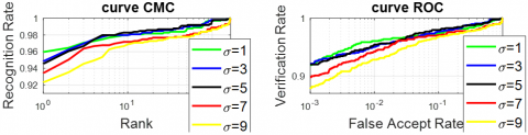
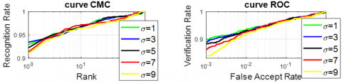
Figure 5. CMC and ROC curves of the RMF modality using xDNN and different deviation values
Table 1 indicates that the best overall identification and verification performance is achieved when the standard deviation σ is set to 1, with a Rank-1 accuracy of 95.96%, an EER of 3.34%, and verification rates of 96.06% and 91.92% at 1% and 0.1% FAR, respectively. Although σ = 5 yields the lowest EER (3.23%) and σ = 3 gives the highest VR at 0.1% FAR (92.12%), these gains are marginal. Therefore, σ = 1 offers the most balanced and consistent performance across all metrics.
Furthermore, the curves CMC and ROC in Figure 5 confirm the best value of the standard deviation of the SQI algorithm. Figure 5 illustrates the results of either reflectance or illuminance on FKP images using the SQI method with several values of ![]() . We can see that the value of 5 fixes the quality of the image.
. We can see that the value of 5 fixes the quality of the image.
In the following part, we look for the best parameters of the PCANet descriptor. Therefore, we fix the value of the standard deviation σ = 1 of the SQI algorithm and analyze the best parameter values of the PCANet descriptor. For that, we have four parameters to test: the overlap ratio (Ra), the filter size (k1, K2), the block size (b), and the number of filters (N).
(a) The overlap ratio (Ra)
We fix the value of the standard deviation at σ = 1, and vary the block overlap ratio (Ra) between 0% (no overlap) and 75%. Table 2 illustrates the results for each value of the overlap ratio in terms of identification accuracy (Rank-1%), Equal Error Rate (EER), and verification performance at 1% and 0.1% FAR thresholds.
Table 2. Results for xDNN and different values of block overlap ratio (Ra) for RMF modality
|
Overlap Ratio (Ra)% |
Identification RANK-1% |
EER% |
VERIFICATION VR@ 1% FAR% |
VERIFICATION VR@ 0.1% FAR% |
|
0 |
91.01% |
5.15% |
91.72% |
86.97% |
|
25 |
94.65% |
3.64% |
94.85% |
91.01% |
|
50 |
93.23% |
3.73% |
94.55% |
90.51% |
|
75 |
94.34% |
3.33% |
95.35% |
91.01% |
From Table 2, we observe that the block overlap ratios Ra = 25% and 75% yield significantly better performance compared to the other values tested. The Ra = 75% configuration achieves the best EER (3.33%) and the highest verification performance at 1% FAR (95.35%), while Ra = 25% produces the best Rank-1 identification accuracy (94.65%) and competitive verification results. Moreover, both Ra = 25% and 75% achieve the highest verification rate at 0.1% FAR, with 91.01%, demonstrating a robust performance in low false acceptance scenarios.
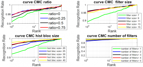
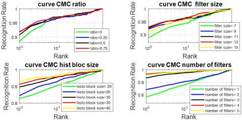
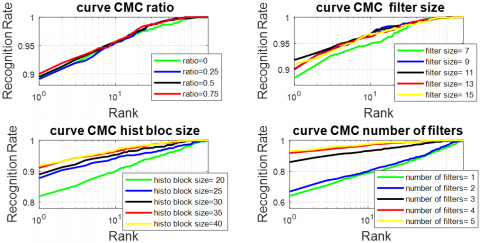
Figure 6. CMC of RMF modality by xDNN and PCANet parameters (ratio,filter size, histobloc size, number of filters)
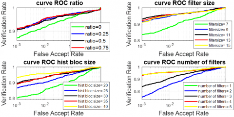
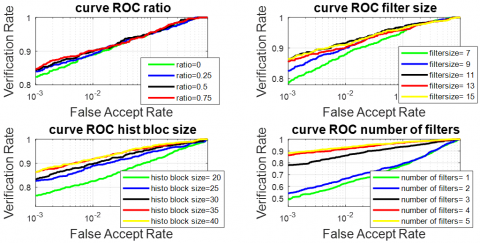
Figure 7. ROC of RMF modality by xDNN and PCANet parameters (ratio,filter size, histobloc size, number of filters)
Figure 6 represents the curve of CMC, and Figure 7 represents the curve of ROC of the FKP recognition system obtained with various values of ratio. In the plot, it can be observed that the values Ra = 25% provide the best performance system.
(b) Filter size (k1, k2) selection
At this stage, the best values previously tested of parameters for the RMF modality are fixed: standard deviation σ = 1 and block overlap ratio Ra = 25%. The goal of this section is to determine the most suitable filter size. In this aim, we evaluate a wide range of filter sizes from (3 × 3) to (15 × 15). Table 3 presents the system performance for each filter size, measured in terms of Rank-1 identification accuracy, Equal Error Rate (EER), and Verification Rates at 1% and 0.1% FAR.
From Table 3, it is clear that the filter size (13 × 13) provides the best overall balance between identification and verification performance. It achieves a Rank-1 identification accuracy of 95.45%, an EER of 3.43%, and the highest verification rate at 0.1% FAR, reaching 95.86%. While the 11×11 filter slightly outperforms it in Rank-1 accuracy (95.96%), the 13×13 filter yields better performance in both verification thresholds, making it the most robust choice.
(c) The bloc Size (b) selection
This section determines the most suitable value for the block size (h) for the RMF-modality, under fixed conditions: standard deviation σ = 1, block overlap ratio Ra = 75%, and filter size (k1, k2) = (13 × 13). We differ the block size between [20, 20] and [40, 40], and estimate the system performance using Rank-1 identification accuracy, Equal Error Rate (EER), and Verification Rates at 1% and 0.1% FAR. The results are presented in Table 4.
Table 4 shows that block size [40, 40] provides the best overall system performance for all evaluation metrics. It achieves the highest rank-1 identification accuracy (95.96%), lowest EER (3.44%), and strong verification results at 1% FAR (95.56%) and 0.1% FAR (93.13%).
(d) Number of filters (N) selection
In this final part, we aim to determine the optimal number of filters (N) for the RMF modality. The number of filters is varied from [1, 1] to [5, 5], while all previously optimized parameters are kept fixed: standard deviation σ = 1, overlap ratio Ra = 75%, filter size (k1, k2) = (13 × 13), and block size b = [40, 40]. The performance results for each filter configuration are shown in Table 5.
From Table 5, it is evident that increasing the number of filters significantly enhances system performance. The configuration [5, 5] achieves the lowest EER (3.33%), the highest verification rates (95.86% at 1% FAR and 93.54% at 0.1% FAR), and matches the top Rank-1 identification accuracy (95.96%). Allowing the Rank-1 value is the same for both [4, 4] and [5, 5], the slight improvement in EER and verification rates makes [5, 5] the most robust choice.
5.4.2 Experimental results for LMF modality
Table 6 reports the performance results of the FKP recognition system for different values of the standard deviation (σ) used in the SQI algorithm, ranging from 1 to 9, for the LMF modality. During this evaluation, all other parameters are kept constant: block overlap ratio Ra = 75%, filter size (k1, k2) = (13 × 13), block size b = [40, 40], and number of filters N = [5, 5].
Table 3. Results for xDNN and different filter sizes (k1, k2) values for RMF modality
|
Filter Size |
Identification RANK-1% |
EER% |
VERIFICATION VR@ 1% FAR% |
VERIFICATION VR@ 0.1% FAR% |
|
3 × 3 |
73.94% |
13.14% |
68.79% |
52.93% |
|
5 × 5 |
85.96% |
8.20% |
83.43% |
75.15% |
|
7 × 7 |
89.09% |
6.78% |
88.08% |
83.54% |
|
9 × 9 |
95.45% |
3.41% |
94.95% |
91.52% |
|
11 × 11 |
95.96% |
3.44% |
95.56% |
93.13% |
|
13 × 13 |
95.45% |
3.43% |
95.86% |
95.86% |
|
15 × 15 |
94.65% |
3.54% |
95.45% |
91.01% |
Table 4. Results for xDNN and different block sizes (b) values for RMF modality
|
Block Size (h) |
Identification RANK-1% |
EER% |
VERIFICATION VR@ 1% FAR% |
VERIFICATION VR@ 0.1% FAR% |
|
[20 20] |
83.43% |
8.88% |
85.25% |
80.00% |
|
[25 25] |
89.60% |
5.55% |
90.10% |
86.46% |
|
[30 30] |
93.13% |
4.45% |
93.43% |
89.49% |
|
[35 35] |
93.64% |
3.94% |
93.23% |
88.89% |
|
[40 40] |
95.96% |
3.44% |
95.56% |
93.13% |
Table 5. Results for xDNN and different number of filters (N) values for RMF modality
|
Number Filters (N) |
Identification RANK-1% |
EER% |
VERIFICATION VR@ 1% FAR% |
VERIFICATION VR@ 0.1% FAR% |
|
[1 1] |
61.41% |
14.74% |
61.01% |
42.12% |
|
[2 2] |
86.87% |
6.66% |
85.35% |
74.95% |
|
[3 3] |
91.72% |
5.16% |
90.91% |
83.54% |
|
[4 4] |
95.96% |
3.44% |
95.56% |
93.13% |
|
[5 5] |
95.96% |
3.33% |
95.86% |
93.54% |
Table 6: Results for xDNN and different values of standard deviation (σ ) values for LMF modality
|
Standard Deviation |
Identification RANK-1% |
EER% |
VERIFICATION VR@ 1% FAR% |
VERIFICATION VR@ 0.1% FAR% |
|
1 |
95.05% |
3.63% |
93.74% |
90.20% |
|
3 |
94.44% |
3.71% |
94.55% |
89.49% |
|
5 |
94.85% |
3.23% |
94.85% |
90.40% |
|
7 |
92.83% |
5.26% |
92.42% |
88.59% |
|
9 |
92.02% |
5.55% |
91.62% |
88.48% |
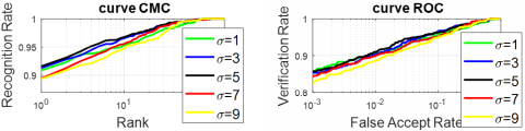
Figure 8. CMC (left) and ROC curves (right) of the LMF modality using different deviation values
From Table 6, we observe that the best system performance is achieved when σ = 5, with a Rank-1 identification rate of 94.85%, the lowest EER of 3.23%, and strong verification performance: 94.85% at 1% FAR and 90.40% at 0.1% FAR. Further, Figure 8 illustrates the CMC and ROC curves of the standard deviation of the FKP recognition system with several values of ![]() It is clearly evident that the
It is clearly evident that the ![]() =5 achieves the best results.
=5 achieves the best results.
Based on these results, we fix the standard deviation at σ = 5 for the LMF modality. In the following sections, we focus on determining the optimal values for the PCANet descriptor parameters, specifically: the overlap ratio (Ra), the filter size (k1, k2), the block size (b), and the number of filters (N).
(a) The overlap ratio (Ra)
In this part, we seek to extract the optimal value of the block overlap ratio (Ra). For that, we take the value of Ra between 0.0% (without overlapping) and 75%, and we calculate the accuracy and the EER. Table 7 presents the results of each value of Ra according to Identification RANK-1%, EER%, Verification VR@ 1% FAR%, and Verification VR@ 0.1% FAR%.
From Table 7, we observe that the block overlap ratio Ra = 75% provides the best overall performance among the tested values. It achieves the lowest EER (4.57%) and the highest verification rate at 0.1% FAR (90.71%), which indicates strong verification performance under strict security constraints. Moreover, it yields 93.33% identification accuracy (Rank-1) and 93.33% verification rate at 1% FAR, which are slightly better than or comparable to the other values. Therefore, the overlap ratio of 75% offers the most balanced and effective trade-off between identification and verification performance.
Table 7. Results for xDNN and different values of overlap ratio (Ra) for LMF modality
|
Block Overlap Ratio (Ra)% |
Identification RANK-1% |
EER% |
VERIFICATION VR@ 1% FAR% |
VERIFICATION VR@ 0.1% FAR% |
|
0 |
91.62% |
5.77% |
91.41% |
85.66% |
|
25 |
93.43% |
4.67% |
93.64% |
89.60% |
|
50 |
92.53% |
5.26% |
92.63% |
88.69% |
|
75 |
93.33% |
4.57% |
93.33% |
90.71% |
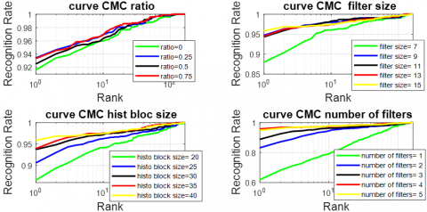
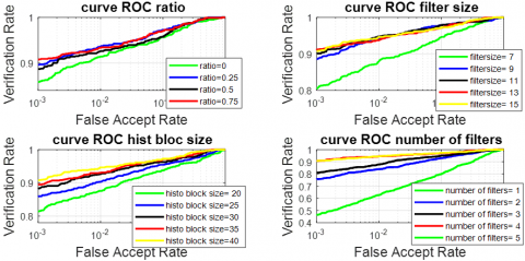
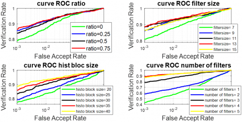
Figure 9 represents the curve of CMC, and Figure 10 represents the curve of ROC of the FKP recognition system obtained with various values of ratio. In the plot, it can be observed that the values Ra = 75% provide the best performance system.
Figure 9. CMC of LMF modality by xDNN and PCANet parameters (ratio, filter size, histobloc size, number of filters)
Figure 10. ROC of LMF modality by xDNN and PCANet parameters (ratio,filter size, histobloc size, number of filters)
(b) Filter size
At this point, the values of different parameters already tested are fixed for the standard deviation σ = 5 and the overlap ratio Ra = 50%. The aim of this part is to select the optimal value for the filter size. The filter size ranges from (3 × 3) to (15 × 15). Table 8 shows the results of each filter.
Table 8. Results for xDNN and different filters size (k1, k2) values for LMF modality
|
Fiter Size |
Identification RANK-1% |
EER% |
VERIFICATION VR@ 1% FAR% |
VERIFICATION VR@ 0.1% FAR% |
|
3 × 3 |
72.02% |
12.95% |
66.06% |
52.42% |
|
5 × 5 |
83.64% |
9.16% |
81.31% |
71.01% |
|
7 × 7 |
87.98% |
6.88% |
88.08% |
80.51% |
|
9 × 9 |
94.75% |
3.74% |
94.14% |
88.59% |
|
11 × 11 |
94.34% |
3.54% |
94.75% |
90.10% |
|
13 × 13 |
94.55% |
4.15% |
93.74% |
91.01% |
|
15 × 15 |
95.86% |
3.83% |
94.65% |
90.71% |
Table 9. Results for xDNN and different block sizes (b) values for LMF modality
|
Block Size (b) |
Identification RANK-1% |
EER% |
VERIFICATION VR@ 1% FAR% |
VERIFICATION VR@ 0.1% FAR% |
|
[20 20] |
86.57% |
6.96% |
87.58% |
81.41% |
|
[25 25] |
90.61% |
5.56% |
90.30% |
85.76% |
|
[30 30] |
93.74% |
4.75% |
92.63% |
88.28% |
|
[35 35] |
93.94% |
4.23% |
93.03% |
89.39% |
|
[40 40] |
95.86% |
3.83% |
94.65% |
90.71% |
We can observe from Table 8 that the filter size 15×15 achieves the best overall system performance in terms of both identification and verification. It yields the highest Rank-1 identification accuracy of 95.86%, and a low EER of 3.83%. Additionally, the verification performance reaches 94.65% at 1% FAR and 90.71% at 0.1% FAR, indicating strong performance under more secure settings. Although the filter size 11×11 offers slightly better EER (3.54%) and 13×13 yields slightly higher VR@0.1% FAR (91.01%), the 15×15 filter size offers the most balanced and robust performance across all criteria.
(c) The block size (b) selection
In this part, we used the previously determined optimal values: standard deviation σ = 5, overlap ratio Ra = 50%, and filter size (k₁, k₂) = (15 × 15). The objective here is to determine the optimal block size for PCANet. To this end, we tested various block sizes ranging from [20, 20] to [40, 40]. Table 9 summarizes the results obtained for each tested configuration.
According to Table 9, the block size [40, 40] achieves the best overall system performance for both identification and verification. It provides the highest Rank-1 identification accuracy of 95.86% and a low EER of 3.83%. Furthermore, the verification rates reach 94.65% at 1% FAR and 90.71% at 0.1% FAR, indicating strong robustness even under stricter verification thresholds. These results confirm that [40, 40] bolck size setting, is the most effective block size setting among those evaluated, offering a good trade-off between spatial resolution and statistical stability in the PCANet framework.
(d) The number of filters
Finally, we tested the impact of varying the number of filters (N) in the PCANet framework. The values were taken from [1, 1] to [5, 5], while keeping the previously optimized parameters fixed: standard deviation σ = 5, overlap ratio Ra = 50%, filter size (k₁, k₂) = (15 × 15), and block size b = [40, 40]. Table 10 presents the results obtained for each configuration.
Table 10. Results for xDNN and different number of filters (N) values for LMF modality
|
Number Filters (N) |
Identification RANK-1% |
EER% |
VERIFICATION VR@ 1% FAR% |
VERIFICATION VR@ 0.1% FAR% |
|
[1 1] |
61.92% |
15.57% |
62.83% |
46.36% |
|
[2 2] |
83.23% |
7.98% |
83.94% |
75.56% |
|
[3 3] |
88.89% |
6.15% |
87.78% |
80.91% |
|
[4 4] |
95.86% |
3.83% |
94.65% |
90.71% |
|
[5 5] |
94.95% |
3.92% |
94.55% |
90.71% |
According to Table 10, the configuration with [4, 4] filters achieves the best system performance in terms of both identification and verification. It yields the highest Rank-1 identification accuracy of 95.86% and the lowest EER of 3.83%, along with 94.65% VR at 1% FAR and 90.71% VR at 0.1% FAR. Although the configuration with [5, 5] filters produces slightly lower accuracy (94.95%) and a marginally higher EER (3.92%), its performance remains comparable. Therefore, the filter number [4, 4] offers the best trade-off between recognition accuracy and computational efficiency in this context.
5.4.3 Experimental results for RIF modality
For the RIF modality, we follow the same evaluation process used for the RMF and LMF modalities. This involves selecting the optimal value for the standard deviation of the SQI algorithm, and then fixing the remaining PCANet parameters: overlap ratio Ra = 75%, filter size (k₁, k₂) = (13 × 13), block size b = [40, 40], and number of filters N = [5, 5]. Table 11 reports the performance results of the FKP recognition system for different values of σ ranging from 1 to 9 under this configuration.
Table 11. Results for xDNN and different values of srandard deviation (σ) for RIF modality
|
Standard Deviation |
Identification RANK-1% |
EER% |
VERIFICATION VR@ 1% FAR% |
VERIFICATION VR@ 0.1% FAR% |
|
1 |
92.93% |
4.45% |
93.43% |
89.60% |
|
3 |
93.43% |
4.46% |
92.73% |
88.89% |
|
5 |
92.22% |
4.64% |
93.03% |
88.08% |
|
7 |
91.31% |
4.34% |
92.53% |
86.06% |
|
9 |
0.9101 |
4.87% |
91.52% |
83.84% |
We observe from Table 11 that the best performance for both identification and verification is achieved when the standard deviation σ = 3, yielding a Rank-1 identification accuracy of 93.43% and an EER of 4.46%. Moreover, at the verification threshold FAR = 0.1%, it reaches 88.89%, and 92.73% at FAR = 1%. While σ = 1 also produces competitive results (92.93% Rank-1, 4.45% EER), the highest identification accuracy is recorded with σ = 3. Further, Figure 11 illustrates the CMC and ROC curves of the standard deviation of the FKP recognition system with several values of σ. It is clearly evident that the σ=5 achieves the best results.
Figure 11. CMC (left) and ROC curves (right) of the RIF modality using different deviation value
(a) The overlap ratio (Ra)
In this part, we aim to determine the optimal value for the block overlap ratio (Ra). To this end, we evaluate Ra values ranging from 0.0% (no overlap) to 75%, and examine the performance in terms of identification accuracy (Rank-1%), Equal Error Rate (EER), and verification rates at 1% and 0.1% FAR. The results are reported in Table 12.
From Table 12, we observe that the best performance is obtained when the block overlap ratio is set to 25%. This setting achieves the highest Rank-1 identification accuracy of 91.92%, and a relatively low EER of 4.65%, along with a verification rate of 91.62% at 1% FAR and 85.45% at 0.1% FAR. Although Ra = 75% achieves a slightly higher VR@1% (92.12%), it comes with a comparable EER (4.65%) and lower Rank-1 accuracy (91.72%) than Ra = 25%. Therefore, based on overall performance across identification and verification, Ra = 25% offers the most balanced and effective configuration in this experiment. Figure 12 represents the curve of CMC, and Figure 13 represents the curve of ROC of the FKP recognition system obtained with various values of ratio. In the plot, it can be observed that the values Ra = 75% provide the best performance system.
(b) Filter size
At this point, the parameters for the RIF modality are fixed: the standard deviation σ = 1 and the overlap ratio Ra = 75%. The objective of this section is to determine the optimal filter size for the PCANet descriptor. To this end, we tested several sizes ranging from (3 × 3) to (15 × 15). Table 13 presents the corresponding performance results based on Rank-1 accuracy, EER, and verification rates.
Table 12. Results for xDNN and different values of block overlap ratio (Ra) for RIF modality
|
Block Overlap Ratio (Ra)% |
Identification RANK-1% |
EER% |
VERIFICATION VR@ 1% FAR% |
VERIFICATION VR@ 0.1% FAR% |
|
0 |
88.48% |
5.65% |
87.17% |
79.09% |
|
25 |
91.92% |
4.65% |
91.62% |
85.45% |
|
50 |
90.71% |
4.43% |
90.81% |
83.94% |
|
75 |
91.72% |
4.65% |
92.12% |
86.57% |
Figure 12. CMC of RIF modality by xDNN and PCANet parameters (ratio,filter size, histobloc size, number of filters)
From Table 13, we observe that the filter size (13×13) delivers the best overall performance in both identification and verification. It achieves the highest Rank-1 identification accuracy of 93.03%, along with the lowest EER of 4.34%. Additionally, it reaches a verification rate of 93.23% at 1% FAR and 88.69% at 0.1% FAR, confirming its robustness even under stricter verification thresholds. Although the (11×11) filter also performs well, (13×13) provides the best balance across all metrics, making it the most suitable filter size for the RIF modality in this configuration.
Figure 13. ROC of RIF modality by xDNN and PCANet parameters (ratio,filter size, histobloc size, number of filters)
(c) The block size (b)
In this part, we aim to select the best block size (h) for the RIF modality, given that the other parameters are fixed as follows: standard deviation σ = 1, overlap ratio Ra = 75%, and filter size (k₁, k₂) = (13 × 13). We vary the block size from [20, 20] to [40, 40], and evaluate the system performance using Rank-1 accuracy, EER, and verification rates. The corresponding results are presented in Table 14.
Table 13. Results for xDNN and different filter sizes (k1, k2) values for RIF modality
|
Fiter Size |
Identification RANK-1% |
EER% |
VERIFICATION VR@ 1% FAR% |
VERIFICATION VR@ 0.1% FAR% |
|
3 × 3 |
60.61% |
15.59% |
55.96% |
42.02% |
|
5 × 5 |
78.99% |
10.75% |
75.86% |
63.74% |
|
7 × 7 |
88.79% |
6.71% |
87.78% |
80.71% |
|
9 × 9 |
92.22% |
5.15% |
91.82% |
86.06% |
|
11 × 11 |
92.63% |
4.95% |
92.93% |
88.48% |
|
13 × 13 |
93.03% |
4.34% |
93.23% |
88.69% |
|
15 × 15 |
91.01% |
5.15% |
91.92% |
86.46% |
Table 14. Results for xDNN and different block sizes (b) values for RIF modality
|
Block Size(h) |
Identification RANK-1% |
EER% |
VERIFICATION VR@ 1% FAR% |
VERIFICATION VR@ 0.1% FAR% |
|
[20 20] |
82.83% |
9.21% |
83.64% |
77.47% |
|
[25 25] |
84.55% |
7.49% |
86.46% |
79.09% |
|
[30 30] |
89.70% |
5.79% |
90.20% |
83.33% |
|
[35 35] |
91.31% |
5.15% |
92.22% |
85.76% |
|
[40 40] |
93.03% |
4.34% |
93.23% |
88.69% |
From Table 14, we observe that the block size [40, 40] achieves the best overall performance in both identification and verification tasks. It records the highest Rank-1 accuracy of 93.03% and the lowest EER of 4.34%, along with 93.23% verification rate at 1% FAR and 88.69% at 0.1% FAR. These improvements confirm that increasing the block size enhances the system’s discriminative capability. Thus, [40, 40] is the most effective block size for the RIF modality in this configuration.
(d) The number of filters
Finally, in this part, we aim to determine the optimal number of filters (N) for the RIF modality. The previously optimized parameters are fixed as follows: standard deviation σ = 1, overlap ratio Ra = 75%, filter size (k₁, k₂) = (13 × 13), and block size b = [40, 40]. We vary the number of filters from [1, 1] to [5, 5], and report the performance metrics in Table 15.
Table 15. Results for xDNN and different number of filters (N) values for RIF modality
|
Number of Filters (N) |
Identification RANK-1% |
EER% |
VERIFICATION VR@ 1% FAR% |
VERIFICATION VR@ 0.1% FAR% |
|
[1 1] |
56.87% |
17.71% |
57.27% |
42.93% |
|
[2 2] |
68.59% |
16.08% |
67.47% |
57.98% |
|
[3 3] |
86.87% |
6.56% |
86.77% |
78.18% |
|
[4 4] |
93.03% |
4.34% |
93.23% |
88.69% |
|
[5 5] |
91.62% |
4.52% |
93.43% |
86.97% |
From Table 15, we observe that the best performance is achieved with [4, 4] filters. This configuration yields the highest Rank-1 identification accuracy of 93.03%, the lowest EER of 4.34%, and excellent verification performance with 93.23% at 1% FAR and 88.69% at 0.1% FAR. Although the setting [5, 5] produces a slightly higher VR@1% (93.43%), it has a lower identification accuracy (91.62%) and a slightly higher EER (4.52%). Therefore, based on the overall balance across all evaluation metrics, the [4, 4] filter configuration provides the most effective performance for the RIF modality.
5.4.4 Experimental Results for LIF modality
Table 16 presents the performance of our biometric image identification and verification system for different values of standard deviation (σ), ranging from 1 to 9, using the LIF modality. In this evaluation, all other parameters are kept fixed: block overlap rate Ra = 75%, filter size (k1, k2) = (13 × 13), block size b = [40, 40], and number of filters N = [5, 5]. The evaluation metrics include rank-1 identification rate, equal error rate (EER), and verification rate (VR) at 1% FAR and 0.1% FAR.
Table 16. Results for xDNN and different values of standard deviation σ for LIF modality
|
Standard Deviation |
Identification RANK-1% |
EER% |
VERIFICATION VR@ 1% FAR% |
VERIFICATION VR@ 0.1% FAR% |
|
1 |
90.91% |
5.26% |
90.71% |
85.76% |
|
3 |
91.31% |
5.17% |
90.40% |
85.35% |
|
5 |
91.62% |
4.85% |
91.01% |
85.66% |
|
7 |
89.49% |
5.76% |
89.80% |
84.34% |
|
9 |
89.39% |
6.53% |
88.69% |
82.63% |
From Table 16, we find σ=5 is optimal for LIF modality, achieving 91.82% Rank-1 accuracy, 4.85% EER, and 91.01% VR@1% FAR with fixed PCANet parameters. Performance declines with lower/higher σ values, confirming σ=5's ideal balance between noise reduction and feature preservation, consistent across all tested modalities. Further, Figure 14 illustrates the CMC and ROC curves of the standard deviation of the FKP recognition system with several values of σ. It is clearly evident that the σ=5 achieves the best results.
Figure 14. CMC (left) and ROC curves(right) of the LIF modality using different deviation value
(a) The overlap ratio (Ra)
We fix the values of the standard deviation σ = 5, and vary the block overlap ratio (Ra) between 0% (no overlap) and 75%. Table 17 shows the performance results of each overlap ratio in terms of identification (Rank-1), Equal Error Rate (EER), and verification accuracy at two different False Acceptance Rates (FARs).
From Table 17, we observe that the best performance is obtained when the block overlap ratio is set to 75%. This setting achieves the highest Rank-1 identification accuracy of (90.00%) and the best verification rates: VR@1% FAR of 90.10% and VR@0.1% FAR of 84.65%. Although the EER is slightly lower at Ra = 50% (5.76%), the overall verification and identification accuracy at Ra = 75% suggest it as the most optimal configuration for the PCANet descriptor under the given settings.
Figure 15 represents the curve of CMC, and Figure 16 represents the curve of ROC of the FKP recognition system obtained with various values of ratio. In the plot, it can be observed that the values Ra = 75% provide the best performance system.
(b) Filter size
In this part, we fix the previously optimized parameters: standard deviation σ = 5 and block overlap ratio Ra = 75%. We now focus on determining the optimal filter size, ranging from (3×3) to (15×15). The performance results of different filter sizes are presented in Table 18.
Table 17. Results for xDNN and different values of block overlap ratio (Ra) for LIF modality
|
Block Overlap Ratio (Ra)% |
Identification RANK-1% |
EER% |
VERIFICATION VR@ 1% FAR% |
VERIFICATION VR@ 0.1% FAR% |
|
0 |
89.19% |
5.96% |
88.89% |
82.32% |
|
25 |
89.09% |
6.04% |
88.99% |
83.94% |
|
50 |
89.49% |
5.76% |
89.80% |
84.34% |
|
75 |
90.00% |
5.98% |
90.10% |
84.65% |
Figure 15. CMC of LIF modality for by xDNN and PCANet parameters (ratio, filter size, histobloc size, number of filters)
Figure 16. Presents the ROC of LIF modality by xDNN and PCANet parameters (ratio, filter size, histobloc size, number of filters)
Table 18. Results for xDNN and different filter sizes (k1, k2) values for LIF modality
|
Fiter Size |
Identification RANK-1% |
EER% |
VERIFICATION VR@ 1% FAR% |
VERIFICATION VR@ 0.1% FAR% |
|
3 × 3 |
91.72% |
5.28% |
91.82% |
87.17% |
|
5 × 5 |
76.46% |
11.22% |
74.65% |
63.33% |
|
7 × 7 |
88.38% |
6.24% |
87.98% |
78.59% |
|
9 × 9 |
90.10% |
4.73% |
90.10% |
82.42% |
|
11 × 11 |
91.82% |
4.44% |
91.62% |
86.36% |
|
13 × 13 |
90.00% |
5.18% |
90.20% |
85.56% |
|
15 × 15 |
91.01% |
4.65% |
91.11% |
86.26% |
From Table 18, we observe that the filter size 11×11 provides the best identification and verification performance, achieving the highest Rank-1 accuracy (91.82%) and the lowest EER (4.44%). Moreover, its verification accuracy at low FARs (VR@0.1% FAR = 86.36%) is also among the top-performing. Therefore, we conclude that the filter size (k1; k2) = (11 × 11) is the most suitable configuration for the PCANet descriptor under the current experimental settings.
(c) The block Size (b)
In this section, we fix the parameters already optimized in previous experiments: standard deviation σ = 5 for the SQI algorithm, overlap ratio Ra = 75%, and filter size (k1; k2) = (11 × 11). We now investigate the effect of different block sizes, ranging from [20, 20] to [40, 40], on the system’s performance. The results of each configuration are presented in Table 19.
From Table 19, we observe that the block size [40, 40] yields the best performance in both identification and verification tasks. It achieves the highest Rank-1 accuracy (91.82%) and the lowest EER (4.44%). The verification rate at VR@0.1% FAR also reaches a strong 86.36%. Based on these results, we confirm that the block size b = [40, 40] offers the most optimal configuration for the FKP recognition system under the current experimental conditions.
(d) The number of filters
Finally, we aim to select the optimal number of filters for the PCANet descriptor applied to the LIF modality. To do this, we test various values of the number of filters N, ranging from [1, 1] to [5, 5], while keeping all previously optimized parameters fixed: standard deviation σ = 5, overlap ratio Ra = 75%, filter size (k1; k2) = (11 × 11), and block size b = [40, 40]. The results are summarized in Table 20.
Table 19. Results for xDNN and different block sizes (b) values for LIF modality
|
Block Size (b) |
Identification RANK-1% |
EER% |
VERIFICATION VR@ 1% FAR% |
VERIFICATION VR@ 0.1% FAR% |
|
[20 20] |
81.92% |
9.51% |
82.53% |
76.57% |
|
[25 25] |
87.78% |
6.77% |
88.99% |
82.63% |
|
[30 30] |
88.99% |
5.47% |
89.70% |
83.33% |
|
[35 35] |
91.11% |
4.55% |
91.72% |
86.26% |
|
[40 40] |
91.82% |
4.44% |
91.62% |
86.36% |
Table 20. Results for xDNN and different number of filters (N) Values for LIF modality
|
Number Filters (N) |
Identification RANK-1% |
EER% |
VERIFICATION VR@ 1% FAR% |
VERIFICATION VR@ 0.1% FAR% |
|
[1 1] |
64.14% |
17.27% |
62.42% |
48.59% |
|
[2 2] |
66.87% |
16.97% |
66.57% |
54.04% |
|
[3 3] |
85.96% |
7.17% |
86.06% |
77.98% |
|
[4 4] |
91.82% |
4.44% |
91.62% |
86.36% |
|
[5 5] |
92.93% |
4.14% |
93.13% |
88.18% |
From Table 20, we observe that increasing the number of filters improves the performance significantly. The configuration N = [5, 5] achieves the best results, with the highest identification rate (Rank-1 = 92.93%), the lowest EER (4.14%), and the best verification performance: VR@1% FAR = 93.13% and VR@0.1% FAR = 88.18%. These results are further illustrated Thus, the number of filters N = [5, 5] is identified as the most optimal choice for the FKP recognition system using PCANet under the given experimental setup.
Table 21 illustrates the summary of all results obtained to select the best value parameters for the SQI algorithm and PCANet descriptor, according to the best values giving for both identification and verification.
Table 21. The best value parameters for the SQI algorithm and PCANet descriptor
|
Parameters |
RMF Modality |
LMF Modality |
RIF Modality |
LIF Modality |
|
Standard deviation σ |
1 |
1 |
3 |
5 |
|
The bloc overlap ratio (Ra) |
25 |
25 |
25 |
75 |
|
Filter Size |
11 × 11 |
15 × 15 |
13 × 13 |
11 × 11 |
|
Bloc size |
[40 40] |
[40 40] |
[40 40] |
[40 40] |
|
Number of Filter |
[5, 5] |
[4, 4] |
[4, 4] |
[5, 5] |
5.5 Comparison study
in this subsection, we compare the proposed system with well-known approaches in the field of Finger-Knuckle-Print (FKP) recognition under a uni-modal configuration. Each finger type (LIF, LMF, RIF, RMF) is treated as an independent modality.
Table 22 presents the identification results, highlighting the superior performance of the proposed framework compared to established methods.
Table 22. ROR (%) the different types fingers
|
Modalities |
ROR (%) |
|
LMF |
95.86 |
|
RMF |
95.96 |
|
LIF |
92.93 |
|
RIF |
93.03 |
To assess the robustness and effectiveness of the proposed illumination-invariant and explainable PCANet-based FKP recognition framework, a comparative study is conducted against several state-of-the-art methods reported in the studies [12, 13, 17, 19]. The evaluation is performed on all four finger categories—Left Index Finger (LIF), Left Middle Finger (LMF), Right Index Finger (RIF), and Right Middle Finger (RMF)—using the same experimental configuration to ensure fairness. The Rank-One Recognition Rate (ROR) was used as the principal performance metric, and the corresponding results are summarized in Table 23.
Table 23. Comparative study between proposed system and other methods
|
Methods |
LIF |
LMF |
RIF |
RMF |
|
ROR (%) |
ROR (%) |
ROR (%) |
ROR (%) |
|
|
Ref [12] |
93.80 |
94.70 |
92.20 |
94.80 |
|
Ref [13] |
91.01 |
94.85 |
91.41 |
91.82 |
|
Ref [17] |
97.30 |
95.75 |
96.83 |
95.15 |
|
Ref [19] |
94.34 |
93.54 |
93.94 |
94.19 |
|
This work |
92.93 |
95.86 |
93.03 |
95.96 |
The obtained results demonstrate that the proposed method achieves a competitive performance across all finger types, with ROR values of 92.93%, 95.86%, 93.03%, and 95.96% for LIF, LMF, RIF, and RMF, respectively. Compared to earlier approaches, the proposed framework maintains a balanced and stable recognition performance, particularly for middle fingers (LMF and RMF), where illumination variations are more pronounced.
Specifically, our method attains the highest ROR values for LMF (95.86%) and RMF (95.96%), surpassing all benchmarked approaches. For LIF and RIF, the system achieves recognition rates of 92.93% and 93.03%, respectively, which are comparable to or slightly lower than the best-reported methods [13, 17]. Overall, the results highlight that our framework not only provides accuracy on par with or superior to state-of-the-art techniques but also introduces a unique advantage in terms of decision transparency, which is absent in conventional black-box models. This combination of competitive accuracy and interpretability establishes our approach as a strong candidate for deployment in security-critical biometric applications.
Although Chlaoua et al. [17] achieve slightly higher RORs on certain finger types, the proposed system provides comparable accuracy while offering enhanced interpretability and illumination robustness, which are not addressed in the compared methods. The integration of the Self-Quotient Image (SQI) preprocessing ensures effective normalization of lighting effects, while the explainable Deep Neural Network (xDNN) component contributes to transparent and interpretable decision-making—a key advantage over purely black-box models.
Overall, the comparative analysis confirms that the proposed framework delivers a strong balance between accuracy, interpretability, and generalization, making it a suitable choice for security-critical biometric systems where both performance and explainability are essential.
Figure 17 presents an example of the interpretable decision rules generated by the proposed xDNN model for retinal image classification. Each condition in the IF–THEN rule corresponds to a prototype (or MegaCloud) that represents a characteristic pattern learned from the training data, thereby providing a transparent link between the input features and the final decision.
Figure 17. Explainability visualization
For instance, Figure 17 illustrates an example of explainability visualization. The rule illustrated as IF (x ∼ Prototype₁) OR (x ∼ Prototype₂) OR (x ∼ Prototype₃) THEN Class = “1” demonstrates how the model associates an input image with one or more representative prototypes. These prototypes are visualized as image patches within the rule, enabling human experts to intuitively understand and visually verify the rationale behind the model’s decision for assigning the input to this specific class.
This visualization offers both objective explainability through the explicit formulation of decision rules—and subjective interpretability through human-readable image prototypes. Such a representation enhances users’ understanding and fosters greater trust in the model’s reasoning process.
Explainable classifier-based biometric systems address the limitations of traditional approaches while achieving superior recognition performance. This paper introduces an innovative xDNN architecture for Finger-Knuckle-Print (FKP) recognition, combining deep learning with full decision transparency. The framework employs a computationally efficient, non-parametric design that eliminates iterative training while maintaining robust performance. By integrating PCANet-based hierarchical feature extraction with illumination-invariant preprocessing via Self-Quotient Images, the system delivers outstanding results on the PolyU FKP database. Experimental validation demonstrates its effectiveness in security-sensitive applications, significantly outperforming conventional methods in both accuracy and interpretability. The system achieves identification accuracies of 91–96% across different finger types while providing fully transparent decision-making, establishing a new benchmark for explainable FKP recognition. Future work will extend this architecture to multi-modal biometrics and hybrid approaches that integrate explainable AI with advanced optimization techniques to enhance robustness and adaptability in real-world deployments. Overall, this study represents an important step toward fully transparent, high-performance FKP recognition systems suitable for modern security applications.
In the future work, we extend the current FKP recognition framework toward multimodal biometric fusion, combining Finger Knuckle Print (FKP) with complementary modalities such as palmprint, fingerprint, and iris to enhance recognition robustness and reliability. Furthermore, we plan to investigate hybrid optimization and feature selection strategies, including metaheuristic-based parameter tuning and deep feature fusion, to improve the adaptability and efficiency of the proposed architecture. These details have been added to provide a clearer and more concrete outlook for future work. Also, we plan to extend this study by conducting a comprehensive user-based evaluation to quantitatively and qualitatively assess the impact of the proposed explainability mechanism on users’ understanding and trust.
Furthermore, this visualization framework combining explicit IF–THEN decision rules with human-readable image prototypes provides both objective explainability and subjective interpretability. This dual representation enhances transparency and fosters greater user confidence in the model’s reasoning process.
[1] Jaswal, G., Nigam, A., Nath, R. (2017). DeepKnuckle: revealing the human identity. Multimedia Tools and Applications, 76(18): 18955-18984. https://doi.org/10.1007/s11042-017-4475-6
[2] Hammouche, R., Attia, A., Akhrouf, S. (2022). Score level fusion of major and minor finger knuckle patterns based symmetric sum-based rules for person authentication. Evolving Systems, 13(3): 469-483. https://doi.org/10.1007/s12530-022-09430-8
[3] Chaa, M., Boukezzoula, N.E., Attia, A. (2017). Score-level fusion of two-dimensional and three-dimensional palmprint for personal recognition systems. Journal of Electronic Imaging, 26(1): 013018. https://doi.org/10.1117/1.JEI.26.1.013018
[4] Qian, J., Yang, J., Tai, Y., Zheng, H. (2016). Exploring deep gradient information for biometric image feature representation. Neurocomputing, 213: 162-171. https://doi.org/10.1016/j.neucom.2015.11.135
[5] Hammouche, R., Attia, A., Akhrouf, S., Akhtar, Z. (2022). Gabor filter bank with deep autoencoder based face recognition system. Expert Systems with Applications, 197: 116743. https://doi.org/10.1016/j.eswa.2022.116743
[6] Cappelli, R., Ferrara, M., Maltoni, D. (2010). Minutia cylinder-code: A new representation and matching technique for fingerprint recognition. IEEE transactions on pattern analysis and machine intelligence, 32(12): 2128-2141. https://doi.org/10.1109/TPAMI.2010.52
[7] Bera, A., Bhattacharjee, D., Nasipuri, M. (2014). Hand biometrics in digital forensics. In Computational Intelligence in Digital Forensics: Forensic Investigation and Applications, pp. 145-163. https://doi.org/10.1007/978-3-319-05885-6_8
[8] Jaswal, G., Kaul, A., Nath, R. (2016). Knuckle print biometrics and fusion schemes--overview, challenges, and solutions. ACM Computing Surveys, 49(2): 34. https://doi.org/10.1145/2938727
[9] Woodard, D.L., Flynn, P.J. (2005). Finger surface as a biometric identifier. Computer Vision and Image Understanding, 100(3): 357-384. https://doi.org/10.1016/j.cviu.2005.06.003
[10] Woodard, D.L., Flynn, P.J. (2005). Personal identification utilizing finger surface features. In 2005 IEEE Computer Society Conference on Computer Vision and Pattern Recognition, San Diego, CA, USA, pp. 1030-1036. https://doi.org/10.1109/CVPR.2005.273
[11] Ferrer, M.A., Travieso, C.M., Alonso, J.B. (2005). Using hand knuckle texture for biometric identification. In Proceedings 39th Annual 2005 International Carnahan Conference on Security Technology, Las Palmas, Spain, pp. 74-78. https://doi.org/10.1109/CCST.2005.1594835
[12] Zeinali, B., Ayatollahi, A., Kakooei, M. (2014). A novel method of applying directional filter bank (DFB) for finger-knuckle-print (FKP) recognition. In 2014 22nd Iranian Conference on Electrical Engineering (ICEE): Tehran, Iran, pp. 500-504. https://doi.org/10.1109/IranianCEE.2014.6999594
[13] Chaa, M., Boukezzoula, N.E., Meraoumia, A. (2018). Features-level fusion of reflectance and illumination images in finger-knuckle-print identification system. International Journal on Artificial Intelligence Tools, 27(3): 1850007. https://doi.org/10.1142/S0218213018500070
[14] Zhang, L., Zhang, L., Zhang, D., Guo, Z. (2012). Phase congruency induced local features for finger-knuckle-print recognition. Pattern Recognition, 45(7): 2522-2531. https://doi.org/10.1016/j.patcog.2012.01.017
[15] Li, Z., Wang, K., Zuo, W. (2012). Finger-knuckle-print recognition using local orientation feature based on steerable filter. In Emerging Intelligent Computing Technology and Applications: 8th International Conference, ICIC 2012, Huangshan, China, pp. 224-230. https://doi.org/10.1007/978-3-642-31837-5_33
[16] Meraoumia, A., Kadri, F., Bendjenna, H., Chitroub, S., Bouridane, A. (2016). Improving biometric identification performance using PCANet deep learning and multispectral palmprint. In Biometric Security and Privacy: Opportunities & Challenges in the Big Data Era, pp. 51-69. https://doi.org/10.1007/978-3-319-47301-7_3
[17] Chlaoua, R., Meraoumia, A., Aiadi, K.E., Korichi, M. (2019). Deep learning for finger-knuckle-print identification system based on PCANet and SVM classifier. Evolving Systems, 10(2): 261-272. https://doi.org/10.1007/s12530-018-9227-y
[18] Angelov, P., Soares, E. (2020). Towards explainable deep neural networks (xDNN). Neural Networks, 130: 185-194. https://doi.org/10.1016/j.neunet.2020.07.010
[19] Attia, A., Akhtar, Z., Chalabi, N.E., Maza, S., Chahir, Y. (2021). Deep rule-based classifier for finger knuckle pattern recognition system. Evolving Systems, 12(4): 1015-1029. https://doi.org/10.1007/s12530-020-09359-w
[20] Benmalek, M., Attia, A., Bouziane, A., Hassaballah, M. (2022). A semi-supervised deep rule-based classifier for robust finger knuckle-print verification. Evolving Systems, 13(6): 837-848. https://doi.org/10.1007/s12530-021-09417-x
[21] Simonyan, K., Zisserman, A. (2014). Very deep convolutional networks for large-scale image recognition. arXiv preprint arXiv:1409.1556. https://doi.org/10.48550/arXiv.1409.1556
[22] Ioffe, S., Szegedy, C. (2015). Batch normalization: Accelerating deep network training by reducing internal covariate shift. In Proceedings of the 32nd International Conference on International Conference on Machine Learning-Volume 37, Lille, France, pp. 448-456.
[23] Angelov, P., Gu, X. (2017). Autonomous learning multi-model classifier of 0-order (ALMMo-0). In 2017 Evolving and Adaptive Intelligent Systems (EAIS): Ljubljana, Slovenia, pp. 1-7. https://doi.org/10.1109/EAIS.2017.7954832
[24] Angelov, P.P., Gu, X. (2019). Empirical Approach to Machine Learning. New York: Springer.
[25] Mlotshwa, T., van Deventer, H., Bosman, A.S. (2022). Cauchy loss function: Robustness under gaussian and Cauchy noise. In Artificial Intelligence Research: Third Southern African Conference, SACAIR 2022, Stellenbosch, South Africa, pp. 123-138. https://doi.org/10.1007/978-3-031-22321-1_9
[26] Varshney, A.K., Torra, V. (2023). Literature review of the recent trends and applications in various fuzzy rule-based systems. International Journal of Fuzzy Systems, 25(6): 2163-2186. https://doi.org/10.1007/s40815-023-01534-w
[27] Markou, M., Singh, S. (2003). Novelty detection: A review—part 2: Neural network based approaches. Signal processing, 83(12): 2499-2521. https://doi.org/10.1016/j.sigpro.2003.07.019
[28] Usha, K., Ezhilarasan, M. (2016). Fusion of geometric and texture features for finger knuckle surface recognition. Alexandria Engineering Journal, 55(1): 683-697. https://doi.org/10.1016/j.aej.2015.10.003
[29] Attia, A., Moussaoui, A., Chaa, M., Chahir, Y. (2018). Finger-knuckle-print recognition system based on features-level fusion of real and imaginary images. Journal on Image and Video Processing. https://doi.org/10.21917/ijivp.2018.0252
[30] Belayadi, Y., Attia, A., Chalabi, N.E., Akhtar, Z., Mohamed, A. W. (2025). Gabor filter bank features selection for face recognition based on particle swarm optimization. Ingénierie des Systèmes d'Information, 30(3): 713-720. https://doi.org/10.18280/isi.300315
[31] Wang, H., Li, S.Z., Wang, Y., Zhang, J. (2004). Self quotient image for face recognition. In 2004 International Conference on Image Processing, 2004. ICIP '04., Singapore, pp. 1397-1400. https://doi.org/10.1109/ICIP.2004.1419763
[32] Muthuraman, D.L., Santhanam, S.M. (2022). Contrast improvement on side scan sonar images using retinex based edge preserved technique. Marine Geophysical Research, 43(2): 17. https://doi.org/10.1007/s11001-022-09478-w
[33] Chan, T. H., Jia, K., Gao, S., Lu, J., Zeng, Z., Ma, Y. (2015). PCANet: A simple deep learning baseline for image classification? IEEE Transactions on Image Processing, 24(12): 5017-5032. https://doi.org/10.1109/TIP.2015.2475625
[34] Xinshao, W., Cheng, C. (2015). Weed seeds classification based on PCANet deep learning baseline. In 2015 Asia-Pacific Signal and Information Processing Association Annual Summit and Conference (APSIPA): Hong Kong, China, pp. 408-415. https://doi.org/10.1109/APSIPA.2015.7415304
[35] PolyU. The Hong Kong polytechnic university (PolyU) Finger-Knuckle-Print Database. https://www4.comp.polyu.edu.hk/~csajaykr/database.php.