Adelia Putri Pangestika![]() | Yenni Angraini*
| Yenni Angraini*![]() | I Made Sumertajaya
| I Made Sumertajaya![]()
© 2025 The authors. This article is published by IIETA and is licensed under the CC BY 4.0 license (http://creativecommons.org/licenses/by/4.0/).
OPEN ACCESS
Anomaly in the air quality index (AQI) is essential to detect as an early warning of air pollution disasters that may occur in the future. Therefore, recognizing the characteristics of anomaly detection methods in AQI data is crucial. This research aims to compare the statistical and deep learning methods in detecting anomalies in the Jakarta AQI data. The data used is Jakarta AQI and calendar variation from January 1, 2019, to February 29, 2024. The method used in this study is a statistical method, namely distributed lag, and a deep learning method, namely autoencoder and LSTM autoencoder, where this method detects anomalies based on the four-sigma rule. The characteristics of anomaly detection using the distributed lag method tend to be more sensitive, with low false negative values and high false positive values. Meanwhile, anomaly detection using the autoencoder method tends to have a high false negative value with a low false positive value. On the other hand, anomaly detection using the LSTM autoencoder method tends to have a low false negative value with a false positive value that is not too high. Considering the characteristics of the methods, the distributed lag method is more recommended.
air quality index, anomaly detection, autoencoder, distributed lag, LSTM autoencoder
An anomaly is an observation that deviates significantly from other observations, giving rise to suspicion that there is a different mechanism that forms the observation. Anomalies are generally viewed as unwanted observations that should be removed. However, anomalies can also be seen as a point of interest that needs to be detected. Anomaly detection has several benefits, namely as a reference for gaining profits and as an early warning of problems that may occur in the future.
Anomaly detection can be done using various approaches, including the time series data approach. Time series data approaches in anomaly detection can be done using various methods, including statistical methods. Anomaly detection using statistical methods has several advantages, including that statistical methods have a clear model basis [1] and have relatively better computational complexity than other methods [2]. However, statistical methods still have several shortcomings. Statistical methods have shortcomings in terms of capturing non-linear patterns in data [3], are unable to model data with high complexity [4] and are only limited to low-dimensional data [5]. One statistical method that can be used is the distributed lag method. Like statistical methods in general, the distributed lag method detects anomalies based on forecasting results. If observations with forecast results are very different from the actual values, then these observations will be detected as an anomaly.
Another anomaly detection method that can be used besides statistical methods is the deep learning method. Deep learning methods can handle nonlinear patterns in high-dimensional data [6], make predictions without creating specific models, and adapt better than statistical methods [7]. However, deep learning methods still have shortcomings in terms of relatively long computing times. Deep learning methods that can be used include the autoencoder method and long short-term memory autoencoder (LSTM autoencoder). The autoencoder and LSTM autoencoder methods detect anomalies based on reconstruction errors, which are the differences between the reconstructed and actual data. When observations with reconstruction errors tend to be large, these observations will be detected as anomalies [8].
Anomalies can occur in various aspects of life, including air conditions. Regarding air conditions, air pollution is becoming a hot issue because it is known to have contributed to 8.8 million deaths in the world [9]. Air pollution is a significant cause of death because it causes various respiratory diseases, such as acute respiratory infections (ARIs). ARIs cases in Jakarta reached 299,721 cases in 2022 and will double to 638,291 cases in 2023 [10]. This doubling of ARIs cases could indicate unusual conditions (anomalies) occurring in the air conditions. Anomalies that occur in air conditions must be watched for, one of which is by monitoring the air quality index.
Anomalies in the air quality index are important to detect as a reference in formulating policies to improve air quality and as an early warning of air pollution disasters that may occur in the future. Jakarta's air quality index data, which is time series data, means that anomaly detection must also be done using a time series data approach. The time series data approach to detect anomalies in the air quality index can be done using statistical methods such as distributed lag and deep learning methods such as autoencoder and LSTM autoencoder.
Statistical methods such as distributed lag have never been used to detect anomalies in time series data. However, this method has quite good forecasting accuracy, so anomaly detection using the distributed lag method is still relevant. The distributed lag method was previously used by the study [11] in forecasting data on cases of death due to COVID-19 in 39 European countries. As a result, this method has good forecasting accuracy, with most median absolute percentage error values below 20%. Meanwhile, deep learning methods such as Autoencoder have been used by the study [12] to detect anomalies in laundry equipment power consumption data. As a result, this method can detect anomalies well and perform better than the isolation forest method. On the other hand, deep learning methods such as LSTM autoencoder were used by the study [13] to detect anomalies in software network data. As a result, this method can detect anomalies effectively and perform better than the one-class support vector machine (OC-SVM) method.
The autoencoder and LSTM autoencoder methods have been proven to detect anomalies effectively and perform better than other methods. However, the performance of these two methods in detecting anomalies has not been compared directly in one study. The performance of these two methods has also never been compared with the statistical method, namely distributed lag. The autoencoder, LSTM autoencoder and distributed lag methods have not been widely used in detecting anomalies in the air quality index. Therefore, this research aims to compare the performance of deep learning methods, namely autoencoder and LSTM autoencoder, with conventional statistical methods, namely distributed lag, in detecting anomalies in the Jakarta air quality index.
2.1 Anomalies in time series data
An anomaly is a data pattern that does not conform to a well-defined notion of normal behavior [14]. The definition of anomaly begins with an outlier [15] is an observation that appears very deviant compared to other observations in a sample. Anomalies can be divided into three types: point anomalies, contextual anomalies, and collective anomalies. A point anomaly occurs when an observation appears significantly deviant from the rest of the observations. Point anomalies can also occur when an observation appears very deviant compared to other observations [16]. Point anomalies were found in extreme heat events during weeks where heavy rain occurred consistently every day. Meanwhile, a contextual anomaly occurs when an observation does not appear deviant compared to other observations as a whole but appears to be deviant when viewed in a particular context. For example, high air humidity is normal if it occurs in the rainy season, but it is anomalous if it occurs in the summer. On the other hand, a collective anomaly occurs when an observation does not appear deviant when observed individually but appears deviant when observed in a group (collectively). For example, high rainfall is normal in the rainy season, but continuous high rainfall is an anomalous condition.
2.2 Distributed lag
The distributed lag method is a method that models response variables not only based on independent variables in the current period but also on independent variables in the previous period [17]. There are two types of distributed lag models: models with infinite lag and models with finite lag. According to the study [18] in Eq. (1), the length of a model with unlimited lag is unknown.
$Y_t=\alpha+\beta_0 X_t+\beta_1 X_{t-1}+\cdots+\varepsilon_t$ (1)
where, $Y_t$ is the value of the response variable for the $t$ period, $\alpha$ is a constant, $\beta$ is the coefficient of the independent variable, and $\varepsilon_t$ is the residual for the t period. In this model, parameter estimation can be done using the koyck method. The koyck method assumes that the further the lag of the independent variable, the smaller its influence on the response variable. This method assumes all $\beta$ coefficients have the same sign and decrease geometrically. Meanwhile, in the model with finite lag, the length of the lag is known as n, as stated in Eq. (2).
$Y_t=\alpha+\beta_0 X_t+\beta_1 X_{t-1}+\cdots+\beta_n X_{t-n}+\varepsilon_t$ (2)
where, $\beta_n$ is the coefficient of the $t-n$ period independent variable, and $X_{t-n}$ is the $t-n$ period independent variable. In this model, parameter estimation can be done using the Almon method. The Almon method assumes the parameter $\beta$ follows a polynomial function.
2.3 Autoencoder
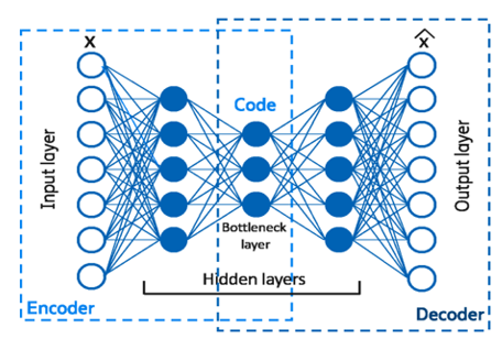
Autoencoder is a method that reduces input into simpler dimensions, called latent dimensions, and reconstructs these latent dimensions into output with the original dimensions [19]. Autoencoder learns important information in the data so that its information can be used to analyze similar data. This method is divided into two parts, the encoder and decoder parts, as shown in Figure 1. The encoder section reduces the input into latent dimensions based on Eq. (3).
$h=f_e\left({W}_e x+b_e\right)$ (3)
where, $h$ is the latent dimension, $f_e$ is the activation function of the encoder section, $W_e$ is the weighting matrix of the encoder section, $x$ is the input vector, and $b_e$ is the bias vector of the encoder section. Meanwhile, the decoder section is tasked with reconstructing the latent dimensions into output with the original dimensions based on Eq. (4).
$\hat{x}=f_d\left({W}_d h+b_d\right)$ (4)
where, $\hat{x}$ is the output, $f_d$ is the activation function of the decoder section, $W_d$ is the weighting matrix of the decoder section, h is the latent dimension, and $b_d$ is the bias vector of the decoder section.
The autoencoder method generally works by minimizing the loss function to form an output as similar as possible to the input [20]. The most commonly used loss function is mean square error (MSE). MSE calculations are carried out based on Eq. (5).
$M S E=\frac{1}{m} \sum_{i=1}^n\left(x_i-\hat{x}_i\right)$ (5)
where, $m$ is the number of observations, $x$ is the input data, and $\hat{x}$ is the output data.
Figure 1. Architecture of autoencoder [21]
2.4 LSTM autoencoder
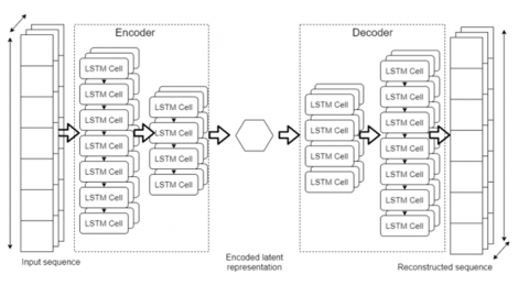
LSTM autoencoder is an anomaly detection method in the form of a combination of the LSTM and autoencoder methods. The LSTM autoencoder method reduces input into more straightforward dimensions or latent dimensions using an LSTM encoder. Next, the latent dimensions are reconstructed into output with the original dimensions using an LSTM decoder [22]. An example of LSTM autoencoder architecture is shown in Figure 2.
Figure 2. Architecture of LSTM autoencoder [23]
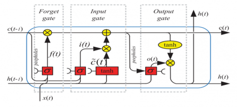
Figure 3. Architecture of LSTM [24]
The LSTM architecture for both the encoder and decoder sections is depicted in Figure 3. In general, LSTM consists of a forget gate, an input gate, and an output gate. Forget gates determine whether information will be used in a process. Meanwhile, the input gate determines the input that will be entered into the cell state memory, and the output gate determines what information will be generated for the new hidden state [25]. The equations used in LSTM are shown by equations below.
$f_t=f\left({W}_f \cdot\left[h_{t-1}, x_t\right]+b_f\right)$ (6)
$i_t=f\left({W}_i \cdot\left[h_{t-1}, x_t\right]+b_i\right)$ (7)
$\tilde{c}_t=f\left({W}_c \cdot\left\lceil h_{t-1}, x_t\right\rceil+b_c\right)$ (8)
$c_t=f_t \times c_{t-1}+i_t \times \tilde{c}_t$ (9)
$o_t=f\left({W}_o \cdot\left[h_{t-1}, x_t\right]+b_o\right)$ (10)
$h_t=o_t \times f\left(c_t\right)$ (11)
where, $f_t$ is the forget gate that uses the sigmoid activation function, $i_t$ is the input gate that uses the sigmoid activation function, $\tilde{c}_t$ is the previous cell state that uses the tanh activation function, $c_t$ is the cell state that has been updated, $o_t$ is the output gate that uses the activation function $\tanh , h_t$ is the new hidden state that uses the tanh activation function, $x_t$ is the input value, $b$ is the bias vector, $W$ is the weighting matrix, and $h_{(t-1)}$ is the previous hidden state.
3.1 Data
The data used is air quality index data (Y) as a response variable and calendar variation data as an explanatory variable (X). This data is recorded in hours and ranges from January 1, 2019 to February 29, 2024. The air quality index data used is sourced from www.airnow.gov, while the calendar variation data used is a dummy variable, which is explained in detail in Table 1.
Table 1. Calender variation data
|
Variable |
Explanation |
|
X1 |
Valued at 1 for weekdays (Monday to Friday) and value at 0 for others |
|
X2 |
Valued 1 for national holidays and value at 0 for others |
|
X3 |
Valued 1 for collective leave and value at 0 for others |
|
X4 |
Valued 1 for seven days before to seven days after Eid Al-Fitr and value at 0 for others |
|
X5 |
Valued 1 for five days before to five days after Eid Al-Fitr and value at 0 for others |
|
X6 |
Valued 1 for three days before to three days after Eid Al-Fitr and value at 0 for others |
|
X7 |
Valued 1 for Eid Al-Fitr and value at 0 for others |
|
X8 |
Valued 1 for Christmas day and value at 0 for others |
|
X9 |
Valued 1 for new year day and value at 0 for others |
|
X10 |
Valued 1 for school holidays and value at 0 for others |
|
X11 |
Valued 1 for Large Scale Social Restriction and value at 0 for others |
|
X12 |
Valued 1 for transitional large scale social restriction and value at 0 for others |
|
X13 |
Valued 1 for Community Activities Restrictions Enforcement (CARE) and value at 0 for others |
3.2 Data preprocessing
Data processing begins by imputing data if there is missing data in several periods. After the missing data has been successfully handled, data exploration is carried out to see patterns and characteristics of the data. Based on the patterns and characteristics of the data, labelling is carried out on the actual data because anomalies in the air quality index data are not labelled naturally. After the actual data is properly labelled, a new dataset that is clean of anomalies is created. This is done because, according to the study [26], the training process for the distributed lag, autoencoder and LSTM autoencoder methods requires a clean dataset of anomalies.
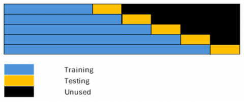
The dataset that is clean from anomalies is then divided into several windows, each consisting of a set of training and test data. The length of the training data in the first window is 1 year and 2 months, while the length of the training data in the next window will increase according to the length of the test data and the window shift distance. The length of the test data and the window shift distance are maintained constant in each window in several scenarios, namely semester, quarter, and trimester. An illustration of the window shift scenario is shown in Figure 4.
Figure 4. Illustration of the window shift scenario
3.3 Anomaly detection using the distributed lag method
For each window in each window shift scenario, anomaly detection using the distributed lag method begins by estimating parameters on the training data. The parameter estimation results in the training data are then used to forecast one period of testing data. These forecast results are then combined with training data and used again in the modelling process to predict the next period. This is done continuously until all test data in a window has forecast results based on the predetermined model.
The forecast results on the test data are then used to calculate the error based on Eq. (12).
$e=\hat{y}-y$ (12)
where, $e$ is the error, $\hat{y}$ is predicted data and $y$ is actual data. Based on this error value, anomaly thresholds are calculated using the $4 \sigma$ rule. In the $4 \sigma$ rule, the upper threshold of the anomaly is calculated based on Eq. (13), while the lower threshold is calculated based on Eq. (14).
$t_u=\bar{e}+4 \sigma_{\text {pooled }}$ (13)
$t_l=\bar{e}-4 \sigma_{\text {pooled }}$ (14)
where, $t_u$ is the upper threshold, $t_l$ is the lower threshold, $\bar{e}$ is the average error value, and $\sigma_{\text {pooled}}$ is composite standard deviation of error that is calculated based on the total sum squared error (SSE) divided by the total degrees of freedom of the entire window. Anomalies are then identified based on these thresholds. Data is identified as an anomaly when the error value exceeds the upper threshold or is less than the specified lower threshold.
3.4 Anomaly detection using the autoencoder and LSTM autoencoder
Anomaly detection using the autoencoder and LSTM autoencoder methods for each window in each window shift scenario begins with standardizing the data. The standardized data is then sequenced and converted into an array in 3D form. Next, the architecture is created, and the hyperparameters that will be used are determined. After the architecture is formed and the hyperparameters are determined, the data training process is carried out on the train data and forecasting on the test data.
The forecast results on the test data are then used to calculate the error based on Eq. (12). The anomaly thresholds are calculated using the $4 \sigma$ rule based on the error value. In the $4 \sigma$ rule, data is identified as an anomaly if the error value is greater than the upper threshold calculated based on Eq. (13) or less than the lower threshold calculated based on Eq. (14).
3.5 Evaluation and comparison of models
Evaluation of anomaly detection results is calculated based on the balance accuracy value. Balanced accuracy shows the average accuracy of the majority and minority classes. According to the study [27], balance accuracy is good when dealing with imbalanced data. The balance accuracy value is then used to compare the anomaly detection results in each window shift scenario using the distributed lag, autoencoder and LSTM autoencoder methods.
4.1 Preprocessing data result
The Jakarta air quality index data consists of 45,264 observations, of which 2,073 are missing. The imputation method used adjusts the characteristics of the missing value encountered. If the missing value period is only one, then the imputation method used is linear interpolation. Suppose the missing value period amounts to more than one period but less than five periods. In that case, the imputation method is adjusted between seasonally decomposed missing value imputation (seadec) and seasonally split missing value imputation (seasplit). If there are more than five consecutive missing value periods, the data imputation process is carried out using daily air quality index data sourced from https://aqicn.org. This daily air quality index has some missing values that are imputed with the forecasting process using the LSTM method. The forecasting process using the LSTM method begins by building a model based on the data available before the appearance of missing values. The model that has been built is then used to predict the value in the first missing period. The forecasting results are then considered as actual data and are reused as input to predict the missing values for the next period. This process is carried out repeatedly until all missing values are successfully predicted. In the forecasting process, 2 LSTM layers and one dense layer are used, each consisting of 50 neuron units. The hyperparameters used in this forecasting process follow the study [28], where this study uses an epoch value of 50, a learning rate of 0.01, a batch size of 72, and a dropout of 0.0. The optimizer used in this forecasting process is the Adam optimizer. After all missing values have been successfully predicted, the imputed daily data is disaggregated into hourly data. Daily data disaggregation is carried out by paying attention to the day the missing value period occurred and using the average air quality index for each hour of that day as a weight.
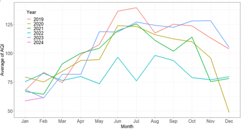
Figure 5. Average of air quality index in every year
After passing the data imputation stage, data exploration uses time series data plots. Data exploration is carried out to see patterns and characteristics of data. Exploratively, the plot of the average air quality index monthly in every year in Figure 5 tends to increase from the beginning to the middle of the year. This increasing pattern is related to the dry season period that occurs in Indonesia. The dry season makes the air drier, with the wind blowing more slowly. This results in no dilution of pollutants in the air, because there are no water droplets trapped in particulates [29]. On the other hand, the average monthly air quality index tends to experience a decreasing pattern in the middle to the end of the year. The decreasing pattern is related to the rainy season period that occurs. The rainy season makes the air tend to be more humid and the wind tends to blow faster. This causes the dilution of pollutants in the air so that the air quality index improves.
Based on the average air quality index pattern monthly in each year, generally, every year has the same pattern except in 2022. In 2022, the average air quality index tends to have a stationary pattern with a lower average value compared to other years. This stationary pattern indicates that unusual conditions (anomalies) occurred that year. The anomaly that occurs is related to the La Nina event, which makes the rainy season prolonged [30].
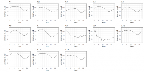
Figure 6. Average of air quality index based on calendar variation
The average air quality index in the hourly period is shown in Figure 6. The air quality index has a pattern that increases at the beginning of the day and peaks at 05.00. The air quality index then experienced a decreasing pattern after that time and had its lowest value at 17.00. After 17.00, the air quality index increased again until the day ended. Fluctuations in the air quality index are closely related to wind patterns in the calm category (<1 m/s). Calm category winds often occur in the morning and cause many pollutants to be trapped near the ground so that pollutant concentrations increase. Meanwhile, in the afternoon, the wind in the calm category tends to be less so that pollutants at the bottom can be blown upwards [31].
Although, in general, the air quality index has a similar pattern every day, there are differences in the pattern in several conditions, such as on Christmas Day (X8) and New Year (X9). On Christmas and New Year’s Day, the air quality index decreases from the beginning of the day until 05.00 and tends to be stationary after that. Apart from that, even though the air quality index has the same pattern in other conditions, there are differences in the range of air quality index values where conditions such as holidays (X2), collective leave (X3) and CARE (X13) have a lower range of air quality index values. This indicates that there are anomalies in these conditions.
Anomalies in the air quality index are naturally not clearly labeled. Considering the pattern of the average air quality index, which rises and falls regularly and slowly, in this study, an anomaly is defined as a data point that suddenly increases or decreases. First, to determine which points are labeled as anomalies, calculate the difference between the air quality index value for the current period $\left(y_t\right)$ and the air quality index for the previous period $\left(y_{t-1}\right)$ based on the Eq. (15).
$d=y_t-y_{t-1}$ (15)
If the difference exceeds $\bar{d} \pm 4 \sigma_d$, then the air quality index data for the current period will be labeled as an anomaly.
A dataset that is clean from anomalies is needed in the model training process using the distributed lag, autoencoder, and LSTM autoencoder methods. To form a dataset free from anomalies, data labeled as an anomaly must be replaced with another value so that the data is no longer an anomaly. In this research, the replacement of data values labeled as anomalies is carried out based on the $d$ value in Eq. (15). If the $d$ value is outside the $4 \sigma_d$ range, then the value will be replaced with the $4 \sigma_d$ threshold based on Eq. (16).
$d^{\prime}= \begin{cases}\bar{d}+4 \sigma_d & \text { if } d>0 \\ \bar{d}-4 \sigma_d & \text { if } d<0\end{cases}$ (16)
Furthermore, the air quality index value for the current period $\left(y_t{ }^{\prime}\right)$ will change according to the Eq. (17).
$y_t^{\prime}=d^{\prime}+y_{t-1}$ (17)
Based on this calculation, changes in the value of $d$ in one period can cause changes in the value of $d$ in the next period. As a result, data initially labeled as normal can be labeled as an anomaly due to changes in the values of $d$ and $y_t$. To overcome this problem, anomaly cleaning is carried out repeatedly until it is ensured that no $d$ values exceed the threshold. The dataset that has been cleaned of anomalies is then ready to be used in the model training process using the distributed lag, autoencoder, and LSTM autoencoder methods. The model training process for the distributed lag, autoencoder, and LSTM autoencoder methods is carried out by dividing the data into several windows with several window-shifting scenarios, namely semester, quarter, and trimester. The anomaly detection process is then carried out based on the forecasting results in each window in each scenario.
4.2 Forecasting results
Forecasting the air quality index using the distributed lag method begins with modeling training data. The modeling results on the training data are used to forecast throughout 1 period of testing data. The results of this forecasting are used again at the modeling stage to carry out forecasts for the next period. This stage is repeated until all testing data in a window has forecast results based on the predetermined model. In the modeling process, seven air quality index variable lags were used by considering the ACF plot and trail error results. During the modeling process, the assumptions of homoscedasticity and normality were violated. This assumption violation is not addressed because the modeling only focuses on point forecasting. This is in accordance with research [32], which states that point forecasts are still relevant even if the homoscedasticity and normality assumptions are violated.
Like the distributed lag method, forecasting using the autoencoder method begins with modeling the training data. The training data is modeled with two dense layers in the encoder section and two dense layers in the decoder section that consists of 128 and 64 neuron units, respectively, with tanh activation functions. The hyperparameters used in the modeling process was carried out based on research by the study [33], where this research uses a batch size value of 32, a learning rate of 0.001, dropout rate of 0.0 and an epoch of 50. The optimizer used in this research is the Adam optimizer. Adam optimizer is used in line with research by the study [34] which states that the Adam optimizer is an efficient optimizer used for forecasting.
Forecasting using the LSTM autoencoder method begins with training data using two LSTM layers in the encoder section and two LSTM layers in the decoder section. Each layer in the encoder and decoder sections consists of 100 neuron units. The hyperparameters used in the LSTM autoencoder method are the same as those used in the autoencoder method. The forecast accuracy results using the distributed lag, autoencoder, and LSTM autoencoder methods are shown in detail in Table 2.
Table 2. Forecasting accuracy of distributed lag, autoencoder, and LSTM autoencoder methods
|
Scenario |
Average MAPE Value (%) |
||
|
Distributed Lag |
Autoencoder |
LSTM Autoencoder |
|
|
Semester |
8.98 $\pm$1.87 |
13.07 $\pm$ 4.09 |
9.33 $\pm$ 1.53 |
|
Quarter |
8.99 $\pm$ 2.60 |
11.31 $\pm$ 3.45 |
9.77 $\pm$ 3.52 |
|
Trimester |
8.99 $\pm$ 2.73 |
11.30 $\pm$ 4.04 |
9.55 $\pm$ 2.66 |
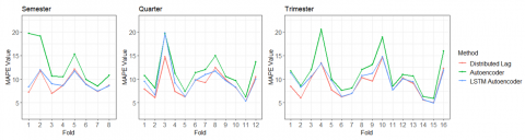
Based on Table 2, both in the semester, quarter, and trimester window shift scenarios, the distributed lag, autoencoder, and LSTM autoencoder methods can predict the air quality index value well, indicated by an average MAPE value of less than 15%. The distributed lag, autoencoder, and LSTM autoencoder methods show similar MAPE value movements between folds, except in the first and fourth folds of the semester scenario, the seventh fold of the quarter scenario, and the ninth fold of the trimester scenario (Figure 7). The distributed lag method is always the method with the best forecasting results compared to other methods. This method also has the most stable inter-fold MAPE value movement in the semester and trimester scenarios. Conversely, the autoencoder method is always the method with the worst forecasting results compared to other methods. This method also has the most unstable inter-fold MAPE value movement in the semester, quarter, and trimester scenarios. Meanwhile, the LSTM autoencoder method is neither the best nor the worst in the three scenarios, but it is the method with the most stable inter-fold MAPE value movement in the quarter scenario.
In the semester window shift scenario, the highest MAPE value of the distributed lag method occurs in the fifth fold, with a value of 12.17%. This is not in line with the autoencoder and LSTM autoencoder methods, where the highest MAPE value of the autoencoder method occurs in the first fold with a value of 19.68%, and the highest MAPE value of the LSTM autoencoder method occurs in the second fold with a value of 11.95%. Meanwhile, the lowest MAPE value in the distributed lag method appears in the third fold with a value of 6.98%. This is not in line with the Autoencoder and LSTM autoencoder methods, which have the lowest MAPE values in the seventh fold. The MAPE values of these two methods in these folds are 8.56% and 7.47%, respectively.
In the quarter window shift scenario, the highest MAPE value of the distributed lag method is in line with the autoencoder and LSTM autoencoder methods, namely in the third fold. In this fold, the MAPE values of the distributed lag, autoencoder, and LSTM autoencoder methods are 14.68%, 19.60%, and 19.74%, respectively. Meanwhile, the lowest MAPE value of the distributed lag method is also in line with the lowest MAPE value of the autoencoder and LSTM autoencoder methods, namely in the eleventh fold. In the eleventh fold, the MAPE values of the distributed lag, autoencoder, and LSTM autoencoder methods are 5.38%, 6.23%, and 5.36%, respectively.
In the trimester window shift scenario, the distributed lag method has the highest MAPE value in the tenth fold, with a value of 14.64%. This is not in line with the autoencoder and LSTM autoencoder methods, where both have the highest MAPE values in the fourth fold, with values of 20.46% and 13.31%, respectively. However, the lowest MAPE value for the distributed lag method occurs in the same fold as the autoencoder and LSTM autoencoder methods, namely in the fifteenth fold. In this fold, the MAPE values of the distributed lag, autoencoder, and LSTM autoencoder methods are 5.04%, 5.94%, and 4.97%, respectively.
Figure 7. Forecast accuracy of distributed lag, autoencoder, and LSTM autoencoder
In general, folds with small MAPE values are folds with forecast error values that tend to be uniform without any error values that are too large. This can indicate the presence of anomalies that are not too steep with a small amount. Meanwhile, folds with large MAPE values can be caused by two possibilities. The first possibility is the presence of observations with huge error values followed by other observations with small error values. This can indicate the presence of steep anomalies with a small amount. The second possibility is the presence of several observations with relatively large error values without being followed by observations with huge error values. This can indicate the presence of anomalies that are not too steep with a large amount.
4.3 Anomaly detection results
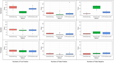
Anomaly detection in the air quality index using the distributed lag, autoencoder, and LSTM autoencoder methods is based on the forecasting results. Data is detected as an anomaly if the forecast error is outside the range of 4 sigma. In the semester window shift scenario, anomaly detection using the distributed lag method produces the largest number of anomalies in the second fold. This does not follow the actual conditions where the second fold is a fold with a small number of anomalies compared to other folds. This condition makes the false positive value of the distributed method in this fold high (Figure 8). Most of the observations that are predicted to be anomalies are not anomalies in actual conditions. This is closely related to the forecasting performance of the distributed lag method, which is further explained in section
However, the false negative value in this fold is the lowest compared to other folds.
In contrast to the distributed lag method, anomaly detection using the autoencoder method produces the largest number of anomalies in the first fold. This follows the actual conditions where the first fold has the largest number of anomalies. However, not all anomalies detected in this fold are anomalies in the actual conditions. This can be seen from the false positive value of the autoencoder method on this fold, which is very high. A very high false negative value accompanies this very high false positive value. The false positive and false negative values on this fold are the highest compared to other folds.
In contrast to the distributed lag and autoencoder methods, anomaly detection using the LSTM autoencoder method produces the largest number of anomalies in the third fold. Although the third fold is a fold with a large number of anomalies, the false positive value of the LSTM autoencoder method in this fold is the highest, even exceeding the false positive values of other methods. This is because the error value in this fold tends to be large and spread out, while the standard deviation of the error used as the anomaly detection threshold is the same for each fold. In line with the autoencoder method, this fold has a very high false positive value and is also accompanied by a high false negative value. This makes the false positive and false negative values in this fold the highest compared to other folds.
In the distributed lag method and LSTM autoencoder, the fifth fold is the least number of anomalies detected in the semester window shift scenario. This follows the actual conditions where the fifth fold has the smallest number of anomalies. In this fold, the very extreme forecast error value makes the anomaly threshold tend to be wider. This makes the detected anomalies more selective, where observations detected as anomalies are indeed anomalies in the actual conditions. As a result, the false positive value in this fold is one of the smallest compared to other folds [35]. The false positive value of the LSTM autoencoder method in this fold even reaches 0.
In contrast to the distributed lag and LSTM autoencoder methods, the smallest number of anomalies detected by the autoencoder method in the semester window shift scenario is in the sixth fold. In this fold, the forecast error value of the autoencoder method is not too large. However, the wide anomaly thresholds make observations whose actual conditions are not correctly detected as anomalies, so the false negative value in this fold tends to be large. However, in this fold, the anomalies detected tend to be more selective, whereas observations detected as anomalies are indeed anomalies in their actual conditions [36]. As a result, the false positive value in this fold reaches 0. Apart from this fold, most of the folds in the semester shift scenario in the autoencoder method have a false positive value of 0.
Figure 8. Confusion matrix of anomaly detection using distributed lag, autoencoder and LSTM autoencoder
In the quarterly window shift scenario, anomaly detection using the distributed lag method produces the largest number of anomalies in the twelfth fold. Meanwhile, anomaly detection using the autoencoder and LSTM autoencoder methods produces the largest number of anomalies in the first and fourth folds, respectively. This is in line with the actual conditions where the twelfth fold owns the largest number of anomalies, the first and fourth fold with the same value of 13. The characteristics of the anomalies detected in the three folds also tend to be the same. All three folds detect anomalies where the anomalies have a high forecast error value without any forecast error value that is too steep. This causes the anomaly boundaries not to be too wide and the number of anomalies detected to be greater. The large number of anomalies detected makes the chance of observations with actual anomalous conditions being detected as anomalies greater so that the false negative value tends to be small. Conversely, the large number of anomalies detected also increases the false positive value, where observations that should be predicted as normal observations are predicted as anomalies [37].
The least number of anomalies in the quarterly window shift scenario occurs in the eighth fold in both the distributed lag, autoencoder and LSTM autoencoder methods. This is in line with the actual conditions where the eighth fold has the smallest number of anomalies. This fold has a very high forecast error value, which makes the anomaly thresholds wider. The wider anomaly thresholds make the anomaly detection process should be more selective, where the observations detected as anomalies are anomalies in their actual conditions. In reality, this only applies to the autoencoder and LSTM autoencoder methods. In the distributed lag method, more than half of the observations detected as anomalies are not anomalies in their actual conditions. However, in the distributed lag method, all data whose actual conditions are anomalous can be perfectly detected as anomalies in the distributed lag method marked with a false negative value of 0.
In the trimester window shift scenario, anomaly detection using the distribution lag method produces the largest number of anomalies in the third fold. Meanwhile, anomaly detection using the autoencoder and LSTM autoencoder methods produces the largest number of anomalies in the fifth fold. This does not align with the conditions where the second fold owns the largest number of anomalies. In the first fold of the distribution lag method and the fifth fold of the autoencoder and LSTM autoencoder methods, the forecast error values produced tend to be high without any forecast error values that are too steep. This causes the anomaly boundaries to tend not to be too wide and the number of anomalies detected to be greater. The large number of anomalies detected makes the chance of observations with actual anomalous conditions being detected as anomalies greater so that false negative values are small and false positives are large.
Anomaly detection using the distribution lag, autoencoder and LSTM autoencoder methods produces the smallest number of anomalies in the tenth fold. This follows the actual conditions where the tenth fold is the fold with the fewest number of anomalies. There is a very extreme forecast error value in this fold, so the anomaly boundaries become wider, and anomaly detection becomes clearer. This should make the observations detected as anomalies indeed anomalies in their actual conditions. In reality, this only applies to the autoencoder and LSTM autoencoder methods. Even the autoencoder method can detect anomalies perfectly without misclassification so that the false negative and false positive values of the autoencoder method on this flip are zero. Meanwhile, in the lag distribution method, most anomalies detected are not anomalies in their actual conditions. Furthermore, the lag distribution and LSTM autoencoder methods can also not detect anomalies well, where these methods classify observations whose actual conditions are anomalous into normal observations.
The measure that can be used to detect anomaly detection results using the lag distribution, autoencoder, and LSTM autoencoder methods is balance accuracy. Balance accuracy is a good measure to use when faced with unbalanced data. The average balance accuracy value for the third method in the third scenario is shown in Table 3.
Table 3. Balance accuracy of distributed lag, autoencoder, and LSTM autoencoder methods
|
Scenario |
Average Balance Accuracy Value (%) |
||
|
Distributed Lag |
Autoencoder |
LSTM Autoencoder |
|
|
Semester |
93.86 $\pm$ 2.38 |
65.64 $\pm$ 7.00 |
87.10 $\pm$ 3.89 |
|
Quarter |
93.73 $\pm$ 3.08 |
85.14 $\pm$ 8.23 |
88.15 $\pm$ 6.24 |
|
Trimester |
92.52 $\pm$ 6.93 |
90.36 $\pm$ 6.87 |
86.38 $\pm$ 7.20 |
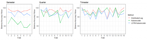
Based on Table 3, the distributed lag method has a higher balance accuracy value than the autoencoder and LSTM autoencoder methods in the semester, quarter and trimester window shift scenarios. The balance accuracy value of the distributed lag method reaches the highest value in the semester window shift scenario and the lowest value in the trimester window shift scenario. In the semester window shift scenario, the distributed lag method generally can detect anomalies well and consistently, indicated by a high balance accuracy value above 89%. In line with the semester window shift scenario, in the quarter window shift scenario, the distributed lag method can detect anomalies well and consistently with the lowest balance accuracy value in the seventh fold with a value of 88.85% and the highest balance accuracy in the eighth fold with a value of 99.93% (Figure 9). Meanwhile, in the trimester window shift scenario, the distributed lag method can generally detect anomalies quite well, where this method has a high balance accuracy value.
However, in the tenth fold, which has the fewest anomalies, the distributed lag method cannot detect anomalies well, as indicated by a balance accuracy value of 74.91%.
Figure 9. Balance accuracy of distributed lag, autoencoder, and LSTM autoencoder
The autoencoder method finds high balance accuracy values in the trimester window shift scenario, followed by the quarter and semester window shift scenarios. In the semester window shift scenario, the highest balance accuracy value is found in the second fold, which aligns with the lowest false negative value. Meanwhile, the lowest balance accuracy value is found in the seventh fold with a high false negative value. In this scenario, the anomaly detection results are not very good, with a balance accuracy value below 80%. Unlike the semester window shift scenario, in the quarter window shift scenario, anomaly detection using the autoencoder method tends to have good results where most folds have a balance accuracy value above 80%. In this scenario, the highest balance accuracy value is owned by the first fold with a value of 96% and the lowest balance accuracy value is owned by the eleventh fold with a value of 77.28%. Meanwhile, in the trimester window shift scenario, there are three folds with perfect detection results with a balance accuracy value of 100%, namely in the seventh, tenth and thirteenth folds. Anomaly detection in this scenario also tends to be consistent, with most folds having a balance accuracy value above 85%. Anomaly detection in this scenario performs better than the LSTM autoencoder method for all scenarios.
In the LSTM autoencoder method, the highest balance accuracy value is found in the quarter window shift scenario. In contrast, the trimester window shift scenario finds the lowest balance accuracy value. This result is inconsistent with the distributed lag and autoencoder methods. Like the distributed lag method, anomaly detection using the LSTM autoencoder method tends to have consistent results marked by the difference in balance accuracy values between folds in each scenario, which is not too high. In the semester window shift scenario, the highest balance accuracy value is found in the first fold, with a value of 90.76%. Meanwhile, the lowest balance accuracy value is found in the seventh fold, at 80.78%. In the quarter window shift scenario, anomaly detection tends to be more consistent than other scenarios. In this scenario, the highest balance accuracy value is found in the first fold, with a value of 96%, while the lowest is found in the eleventh fold, at 77.26%. Meanwhile, in the trimester window shift scenario, the LSTM autoencoder method can detect anomalies almost perfectly with a balance accuracy value of 99.84%, namely in the first fold. However, this method can detect anomalies in other folds quite consistently, with the lowest balance accuracy value being in the fourth fold, which has a value of 74.95%. In the trimester window shift scenario, the autoencoder method tends to have a small balance accuracy value in folds with a small number of anomalies.
4.4 Comparison of distributed lag, autoencoder, and LSTM autoencoder methods in detecting anomalies in the air quality index
The forecasting ability of each method dramatically influences the ability to detect anomalies. The method with the highest forecasting capability, in this case, distributed lag, has anomaly thresholds that tend to be narrower than other methods. This makes anomaly detection more sensitive, and more anomalies are detected. The large number of anomalies detected means that the chances of an observation whose actual condition is an anomaly being detected as an anomaly also becomes higher. As a result, the false negative value for this method tends to be lower, while the balance accuracy value tends to be higher. However, the number of anomalies detected does not necessarily reflect the actual conditions. In the distributed lag method, the majority of the many observations detected as anomalies are not anomalies in actual conditions. This causes the distributed lag method’s false positive value to be higher than other methods. The distributed lag method tends to have good performance with high balance accuracy values on folds with a large number of actual anomalies. Folds like this usually have anomalous characteristics that are not too steep. On the other hand, this method tends to perform less well on folds with a small number of actual anomalies.
In methods with forecasting capabilities that tend to be less suitable than other methods, in this case, the autoencoder method, the anomaly thresholds tend to be wider because the variety of forecasting errors tends to be larger. This causes anomaly detection to be less sensitive and the number of anomalies detected to be fewer. However, the high anomaly thresholds and the small number of anomalies make the autoencoder method tend to be more selective in detecting anomalies. Observations detected as anomalies are indeed anomalies in actual conditions. This makes the false positive value for this method smaller than that of other methods. Most of the folds in this method have a false positive value of zero. However, the wide range of anomaly detection makes this method less suitable for detecting not too steep anomalies. As a result, there are observations whose actual conditions are anomalies classified as normal observations. This makes the false negative value for this method tend to be high, accompanied by the balance accuracy value, which tends to be low. However, this method is quite suitable for detecting anomalies in folds with a few actual anomalies with steep anomaly characteristics. The balance accuracy value of the autoencoder method on folds with these characteristics reaches 100%.
In the LSTM autoencoder method, the forecasting ability at each fold of this method is better than the autoencoder method but not better than the distributed lag method. The anomaly threshold of this method is also quite wide, where this method has a wider anomaly threshold than the distributed lag method but not wider than the autoencoder method. This causes the number of detected anomalies to be quite large. The large number of anomalies detected makes the chance of an observation in which the actual condition of the anomaly being detected as an anomaly becomes greater so that the false negative value tends to be low and the balance accuracy value tends to be high. However, this does not necessarily make the false positive value of this method high. In several folds in the three scenarios, the false positive value for this method reached 0. However, several folds were also found with very high false positive values. This is because the error in the fold is relatively large and spread out, while the standard deviation of error used as a threshold in anomaly detection is set the same for each fold. The LSTM autoencoder method works well on folds with anomalous characteristics that are not too steep and have many anomalies.
The distributed lag method has excellent forecasting performance with anomaly thresholds that tend to be narrow. Anomaly detection using this method tend to be more sensitive, with low false negative values and high false positive values. This method is suitable for anomaly detection with no steep characteristics. Meanwhile, the autoencoder method has a forecasting performance that is not very good compared to other methods. Anomaly detection using this method tends to have a high false negative rate with a very low false positive rate. This method is suitable for detecting anomalies with steep characteristics. On the other hand, the LSTM autoencoder method has better forecasting performance than the autoencoder method but not better than the distributed lag method. This method has a false negative rate, which tends to be low, and a false positive rate, which is not too high. This method is quite suitable for both anomalies with characteristics that are not too steep and detect anomalies with quite steep characteristics.
Anomaly detection in this study is only limited to air quality index data. Air quality index data has characteristics that may differ from other data. The characteristics of anomaly detection methods in air quality index data cannot necessarily be generalized to other datasets. To generalize the characteristics of the three anomaly detection methods, further research can be carried out on simulated data generated with various scenarios.
This research was supported by grants from BIMA-Ministry of Education, Culture, Research and Technology of Republic of Indonesia with contract number 027/E5/ PG.02.00.PL/2024.
[1] Kozitsin, V., Katser, I., Lakontsev, D. (2021). Online forecasting and anomaly detection based on the ARIMA model. Applied Sciences, 11(7): 3194. https://doi.org/10.3390/app11073194
[2] Ahmed, M., Mahmood, A.N., Hu, J. (2016). A survey of network anomaly detection techniques. Journal of Network and Computer Applications, 60: 19-31. https://doi.org/10.1016/j.jnca.2015.11.016
[3] Jeong, K.J., Shin, Y.M. (2022). Time-series anomaly detection with implicit neural representation. arXiv preprint arXiv:2201.11950. https://doi.org/10.48550/arXiv.2201.11950
[4] Kundu, A., Sahu, A., Serpedin, E., Davis, K. (2020). A3D: Attention-based auto-encoder anomaly detector for false data injection attacks. Electric Power Systems Research, 189: 106795. https://doi.org/10.1016/j.epsr.2020.106795
[5] Zhang, J. (2013). Advancements of outlier detection: A survey. ICST Transactions on Scalable Information Systems, 13(1): 1-26. https://doi.org/10.4108/trans.sis.2013.01-03.e2
[6] Lin, S., Feng, Y. (2022). Research on stock price prediction based on orthogonal gaussian basis function expansion and pearson correlation coefficient weighted LSTM neural network. Advances in Computer, Signals and Systems, 6(5): 23-30. https://doi.org/10.23977/acss.2022.060504
[7] Meng, X.R., Chang, H.Q., Wang, X.Q. (2022). Methane concentration prediction method based on deep learning and classical time series analysis. Energies, 15(6): 2262. https://doi.org/10.3390/en15062262
[8] Belay, M.A., Blakseth, S.S., Rasheed, A., Salvo Rossi, P. (2023). Unsupervised anomaly detection for IoT-based multivariate time series: Existing solutions, performance analysis and future directions. Sensors, 23(5): 2844. https://doi.org/10.3390/s23052844
[9] Janarthanan, R., Partheeban, P., Somasundaram, K., Elamparithi, P.N. (2021). A deep learning approach for prediction of air quality index in a metropolitan city. Sustainable Cities and Society, 67: 102720. https://doi.org/10.1016/j.scs.2021.102720
[10] Situmeang, B.S., Napitupulu, R., Ambu, R.S., Yohanes, A., Yoshua, S., Siahaan, C. (2023). Pengaruh tingkat polusi udara terhadap tingkat pengidap penyakit ispa di lingkup masyarakat kramat jati. Journal of Comprehensive Science (JCS): 2(12): 1520-1539.
[11] Hadianfar, A., Rastaghi, S., Tabesh, H., Saki, A. (2023). Application of distributed lag models and spatial analysis for comparing the performance of the COVID-19 control decisions in European countries. Scientific Reports, 13(1): 17466. https://doi.org/10.1038/s41598-023-44830-z
[12] Alfeo, A.L., Cimino, M.G., Manco, G., Ritacco, E., Vaglini, G. (2020). Using an autoencoder in the design of an anomaly detector for smart manufacturing. Pattern Recognition Letters, 136: 272-278. https://doi.org/10.1016/j.patrec.2020.06.008
[13] Said Elsayed, M., Le-Khac, N.A., Dev, S., Jurcut, A.D. (2020). Network anomaly detection using LSTM based autoencoder. In Proceedings of the 16th ACM Symposium on QoS and Security for Wireless and Mobile Networks, New York, United States, pp. 37-45. https://doi.org/10.1145/3416013.3426457
[14] Chandola, V., Banerjee, A., Kumar, V. (2009). Anomaly detection: A survey. ACM Computing Surveys (CSUR), 41(3): 1-58. https://doi.org/10.1145/1541880.1541882
[15] Grubbs, F.E. (1969). Procedures for detecting outlying observations in samples. Technometrics, 11(1): 1-21. https://doi.org/10.1080/00401706.1969.10490657
[16] Blázquez-García, A., Conde, A., Mori, U., Lozano, J.A. (2021). A review on outlier/anomaly detection in time series data. ACM Computing Surveys (CSUR), 54(3): 1-33. https://doi.org/10.1145/3444690
[17] Corlett, W.J. (2003). Basic econometrics. The Economic Journal, 82(326): 770-772. https://doi.org/10.2307/2230043
[18] Porter, D.C. (2009). Basic econometrics. In Introductory Econometrics: A Practical Approach. Douglas Reiner.
[19] Que, Z.Q., Liu, Y.Y., Guo, C., Niu, X.Y., Zhu, Y.X., Luk, W.Y. (2019). Real-time anomaly detection for flight testing using AutoEncoder and LSTM. In 2019 international conference on field-programmable technology (ICFPT), Tianjin, China, pp. 379-382. https://doi.org/10.1109/ICFPT47387.2019.00072
[20] Pinaya, W.H.L., Vieira, S., Dias, R.G., Mechelli, A. (2019). Chapter 11 — Autoencoders. Machine Learning Methods and Applications to Brain Disorders. Academic Press, United States, pp. 193-208. https://doi.org/10.1016/B978-0-12-815739-8.00011-0
[21] Salahuddin, M.A., Bari, M.F., Alameddine, H.A., Pourahmadi, V., Boutaba, R. (2020). Time-based anomaly detection using autoencoder. In 2020 16th International Conference on Network and Service Management (CNSM), Izmir, Turkey, pp. 1-9. https://doi.org/10.23919/CNSM50824.2020.9269112
[22] Nguyen, H.D., Tran, K.P., Thomassey, S., Hamad, M. (2021). Forecasting and anomaly detection approaches using LSTM and LSTM autoencoder techniques with the applications in supply chain management. International Journal of Information Management, 57: 102282. https://doi.org/10.1016/j.ijinfomgt.2020.102282
[23] Venskus, J., Treigys, P., Markevičiūtė, J. (2021). Unsupervised marine vessel trajectory prediction using LSTM network and wild bootstrapping techniques. Nonlinear Analysis: Modelling and Control, 26(4): 718-737. https://doi.org/10.15388/namc.2021.26.23056
[24] Yu, Y., Si, X.S., Hu, C.H., Zhang, J.X. (2019). A review of recurrent neural networks: LSTM cells and network architectures. Neural Computation, 31(7): 1235-1270. https://doi.org/10.1162/neco_a_01199
[25] Van Houdt, G., Mosquera, C., Nápoles, G. (2020). A review on the long short-term memory model. Artificial Intelligence Review, 53(8): 5929-5955. https://doi.org/10.1007/s10462-020-09838-1
[26] Kirichenko, L., Koval, Y., Yakovlev, S., Chumachenko, D. (2024). Anomaly detection in fractal time series with LSTM autoencoders. Mathematics, 12(19): 3079. https://doi.org/10.3390/math12193079
[27] Grandini, M., Bagli, E., Visani, G. (2020). Metrics for multi-class classification: An overview. arXiv preprint arXiv:2008.05756. https://doi.org/10.48550/arXiv.2008.05756
[28] Huang, Y., Yu, J.H., Dai, X.H., Huang, Z., Li, Y.Y. (2022). Air-quality prediction based on the EMD–IPSO–LSTM combination model. Sustainability, 14(9): 4889. https://doi.org/10.3390/su14094889
[29] Ahmad, E.F., Santoso, M. (2016). Analisis karaterisasi konsentrasi dan komposisi partikulat udara (Studi case: Surabaya). Jurnal Kimia Valensi, 2(2): 97-103. http://dx.doi.org/10.15408/jkv.v0i0.3602
[30] Harahap, W.N., Yuniasih, B., Gunawan, S. (2023). Dampak la nina 2021-2022 terhadap peningkatan curah hujan. AGROISTA: Jurnal Agroteknologi, 7(1): 26-32. https://doi.org/10.55180/agi.v7i1.364
[31] Hutauruk, R.C.H., Rahmanto, E., Pancawati, M.C. (2020). Variasi musiman dan harian PM2.5 di Jakarta periode 2016-2019. Buletin GAW Bariri, 1(1): 20-28. https://doi.org/10.31172/bgb.v1i1.7
[32] Knaub Jr, J.R. (2021). When would heteroscedasticity in regression occur? Pakistan Journal of Statistics, 37(4): 315-367.
[33] Shakir, M., Kumaran, U., Rakesh, N. (2024). An approach towards forecasting time series air pollution data using LSTM-based auto-encoders. Journal of Internet Services and Information Security, 14(2): 32-46. https://doi.org/10.58346/JISIS.2024.I2.003
[34] Reyad, M., Sarhan, A.M., Arafa, M. (2023). A modified Adam algorithm for deep neural network optimization. Neural Computing and Applications, 35(23): 17095-17112. https://doi.org/10.1007/s00521-023-08568-z
[35] Zhang, Y.M., Wang, H., Wan, H.P., Mao, J.X., Xu, Y.C. (2021). Anomaly detection of structural health monitoring data using the maximum likelihood estimation-based Bayesian dynamic linear model. Structural Health Monitoring, 20(6): 2936-2952. https://doi.org/10.1177/1475921720977020
[36] Schlechtingen, M., Santos, I.F. (2011). Comparative analysis of neural network and regression based condition monitoring approaches for wind turbine fault detection. Mechanical Systems and Signal Processing, 25(5): 1849-1875. https://doi.org/10.1016/j.ymssp.2010.12.007
[37] Choi, K., Yi, J.H., Park, C., Yoon, S. (2021). Deep learning for anomaly detection in time-series data: Review, analysis, and guidelines. IEEE Access, 9: 120043-120065. https://doi.org/10.1109/ACCESS.2021.3107975