Harmanjeet Singh![]() | Preeti Sharma*
| Preeti Sharma*![]() | Chander Prabha
| Chander Prabha![]() | Meenakshi
| Meenakshi![]() | Supreet Singh
| Supreet Singh![]()
© 2024 The authors. This article is published by IIETA and is licensed under the CC BY 4.0 license (http://creativecommons.org/licenses/by/4.0/).
OPEN ACCESS
AI has increased scholarly interest in predicting financial stock prices, a tough task. Recurrent neural network (RNN) time series price movement analysis is common but ignores market, investor, and headline factors. Graph neural networks excel at capturing complicated relationships and learning representations, making them useful for a variety of applications. This study investigates the predictive capabilities of graph neural networks about stock prices. Recent studies motivated to utilize hypergraphs for capturing intricate group-level data, such as corporate mobility patterns. Using a graph model to obtain paired linkages sets us apart from previous studies on hypergraphs. Also, demonstrated that using RNNs after applying this fundamental graph model is not advisable, in contrast to previous research. This study demonstrates the potential of future Recurrent Neural Networks (RNNs) to acquire knowledge about the long-term interconnections across companies, leading to enhanced predictive capabilities. The proposed model is an innovative ensemble learning framework that created specifically for the purpose of forecasting stock values. Part, one consists of a Graph Convolution Network (GCN), which encodes price and industry pairs. Part two involves a hypergraph convolution network that conducts adversarial training by modifying inputs before the final prediction layer. This modification facilitates the transmission of group-oriented information through hyperedges. There is empirical evidence that suggests that the proposed model outperforms approaches that are considered to be state-of-the-art on average and demonstrates remarkable performance during times when the market is declining. The proposed framework beats the second-best baseline by increments of 1.14%, 3.63%, and 2.45% for three different five-days, ten days and twenty days trade periods.
adversarial hypergraph model, artificial intelligence, ensemble learning, machine learning, neural network, recurrent unit stock price forecast, time series
Stock prediction has long been studied, and investors are always seeking for methods to enhance their models. Research reveals that industry information may accurately anticipate the entire stock market with a two-month time horizon, despite the fact that regulations and societal factors something like global epidemics can have a tremendous effect on the financial sector, which makes it difficult to make accurate predictions about stock prices [1]. Equities within an industry behave differently from those outsides of it. Therefore, they are crucial relational components for complete integration. A good tool for this job is graph neural networks (GNNs), which leverage network structure [2]. Yes, there have been some initial, limited alternatives. For the purpose of predicting the price of stocks and other data pairs to be traded the following day, modern GNNs use simple graphs to depict these paired relations. More complex theories are needed to explain such conduct, but comparable company stock values tend to move together. Consequently, the authors propose using hypergraphs1 to model business- and fund-level stock linkages (shared funds being investors). In spite of the fact that they are effective on basic graphs, the present generation of GNNs is unable to take advantage of the high-order structure of hyperedges, and deep learning on hypergraphs is still in its infancy [3]. Sawhney et al. [4] suggested tracking stock patterns with hypergraphs with gated temporal convolution. Cui et al. [5] forecast stock price movement using hypergraph attention networks and found that hypergraphs capture similar stock patterns. They considered group-level analysis but ignored financial market pairwise correlations between comparable organizations. According to Aghabozorgi and Teh [6], similar patterns of volatility may be observed in equities that belong to the same industry. 1 is an illustration of this concept. The stocks of Ningbo Bank (NB), China Merchants Bank (CMB), and Bank of China are displayed in this chart, which uses data from several sources. This photograph lends credence to their assertion. With the use of this formula, it is possible to find the degree of correlation for both stock prices:
$R_{x y}=\frac{\sum_{k=1}^n\left(x_i-\hat{x}\right)\left(y_i-\hat{y}\right)}{\sqrt{\sum_{k=1}^n\left(x_i-\hat{x}\right)^2\left(y_i-\hat{y}\right)^2}}$
One method for determining the degree of association between two stocks is to examine their correlation coefficient. Typically positioned within a moderate range, the value might range from -1 to 1. The condition of a “perfectly” connected relationship between two securities is met when their correlation coefficients are both equal to 1. When one stock increases by five points, the other stock also increases by five points precisely at the same time. An “ideal” inverse relationship is shown by a correlation coefficient of -1, when a five-point increase in one stock is accompanied by a corresponding decrease of the other one. Due to the infrequency of such occurrences within the stock market, the notion of perfect correlations is predominantly confined to academic circles.
NB and CMB have a 0.72 correlation value, whereas NB and BOC have 0.64. One possible explanation for the considerable relationship between the two pairings is that the same mutual fund will own both from September 30, 2020, to December 31, 2020. As a result, the authors anticipate the presence of pairwise links in more equities within the same sector and owned by the same investment vehicle. Before employing the use of recurrent neural networks (RNNs), a graph neural network is utilized to add industry and pricing data to improve the pairwise behavior of related firms. In the study by Berk et al. [7], despite the fact that the authors utilize GCN initially, the authors make the assumption that price movement is linear or steady. This allows RNNs to accurately depict the long-term dependency of paired organizations [8]. Since it is a component of the hypergraph convolution, the authors are avoiding processing fund-holding data through the GCN. Due to the diverse asset classes that mutual funds are required to hold; fund-holding data has a lower significance in determining the value of individual stocks than industry data [9]. However, it’s not always a poor predictor of market trends. To sum up, the suggested approach is capable of pairwise and group-level analysis of dynamic historical price data among fund-held firms in the same industry.
Financial market price fluctuations are stochastic, hence standard training may overfit. Thus, the authors want to know:
Our solution is hypergraph convolution with adversarial training, which accounts for disrupted features and incorporates an adversarial loss into the loss of computation. The authors employ voting ensemble learning and the highest vote count to separate predicted classes from adversarial and conventional training. In summary, the paper contributes:
2.1 GNN for price prediction
Attempts have been made by researchers to express stock relations as graphs in order to train GNNs to learn stock representations [10]. To acquire knowledge on shareholding information, a hybrid technique consisting of Graph Convolutional Networks (GCN) and Long Short-Term Memory (LSTM) was utilized. Subsequently, the study by Xiong et al. [11] a multi-graph convolution network was utilized to forecast stock value variations. This network gave equal weight to graphs that depicted stock ownership, industry, and news links.
In light of recent recommendations made by academics, it has been suggested that the correlations between stock prices and other pertinent data can be depicted using a variety of graphs. The study by Guo [12] a diversified graph was constructed by making use of data at the event level as well as contextual information for the goal of forecasting stock performance. Singh et al. [13] proved that hypergraphs can capture complicated relationships between stocks on a group level of data. The study utilized a hypergraph convolutional network to accurately represent the relationship between fund-holding and business activities and stock volatility. In addition to the financial industry, hypergraph neural networks have demonstrated their usefulness. Their expertise in the disciplines of recommendation and learning analytics was demonstrated in multiple studies that were conducted recently, including [14, 15]. These studies provide valuable insights for readers seeking to observe the application of hypergraph modelling in diverse businesses and broader contexts.
While the aforementioned financial prediction approaches proved to be effective, most of them relied on recurrent neural network (RNN) models that just utilized historical stock price data to generate new price embeddings. Subsequently, employing GCN or an alternative graph neural network, the revised embedding can be subjected to further analysis alongside additional components, such as news [16], industry [17], or shareholder information [18]. In addition, it is worth considering affiliated enterprises [19]. However, the post-processing was conducted at an inconvenient moment. These approaches were limited since they depended on RNN as a starting point and could only capture pairwise connections between stocks. They assumed that all other historical data is linear or steady. Previous hypergraph models disregarded these specific pairwise characteristics while overemphasizing group-level interactions [20].
Furthermore, it is worth noting that none of these research studies fully addressed the issue of overfitting, which in this particular scenario is produced by the constantly shifting market conditions.
2.2 Adversarial training
Significant focus has lately been placed on it [21], as it is undoubtedly the most efficient approach for enhancing model generalization by "protecting" against distorted data. Even when confronted with adversarial attacks, the major goal of adversarial training is to ensure that models continue to generate accurate results while preserving their consistency. This can be accomplished through the combination of negative examples and clean data. Managing overfitting resulting from the market's erratic and ever-changing characteristics is necessary for forecasting stock price fluctuations. In the study by Singh and Malhotra [22], adversarial training on commercial interval insights was performed, and the random characteristics of stock features were successfully recreated. Specifically, Chawla and Walia [23] introduced a sentiment-guided generative adversarial network to address the topic of stock prediction. With the goal of achieving results that are competitive, Jaswal et al. [24] integrated adversarial training with transfer learning.
2.3 Ensemble learning for price prediction
Convolutional neural networks, often known as CNNs, are currently being utilized in the study of price forecasting to improve the accuracy of classification or regression by applying deep learning techniques. In the analysis of financial time series, the research carried out by the study of Baghel et al. [25] showed that the combined models had excellent performance compared to the separate models they were compared to. Using denoising autoencoders (SDAE) with bootstrap aggregation (bagging), as proposed by Singh and Malhotra [26], is one method for accurately depicting the intricate interrelationships between oil price and its variables. To forecast the S&P 500 index, this study used a combination of ensemble learning and two RNNs in the study by Chen et al. [27]. The framework for forecasting stock indexes established by the study of Ye et al. [28] included four tree-based ensemble algorithms: XGBoost, LightGBM, vanilla RNN, bidirectional RNN, LSTM, and gated recurrent unit (GRU).
Standard training may lead to overfitting in the dynamic financial market with stochastic price movements. So, the research questions are:
Question 1: Is it possible to improve stock price forecasts by collecting complicated business data?
Question 2: How can we make the model more resilient without lowering its accuracy in prediction?
To answer the questions, combining hypergraph convolution and essential grid learning can effectively detect complicated linkages across identical stocks while addressing stock stochasticity via adversarial training. This approach has promise for addressing the aforementioned inquiries. In contrast to alternative approaches that initially employ recurrent neural networks (RNNs), the authors demonstrated the efficacy of integrating supplementary information, such as industry data, through a Graph Convolutional Network (GCN) prior to utilizing RNNs. This enables Recurrent Neural Networks (RNNs) to comprehend the enduring interdependencies of pairwise relationships among comparable organizations in the future.
3.1 Problem formulation
This analysis predicts stock movements for the next trading day. According to the study of Xiong et al. [29], stock prices can move upward, stabilize, or decrease from the previous trading day. Funds FS, industry traits IS, and ordinary transactions from the past XS inform our analysis. This information is crucial for 5, 10, and 20-day trades. According to a previous study [18], a one-point gain means the stock’s closing price the next trading day $P_t$ is at least 0.55% higher than the day before $P_{t-1}$.
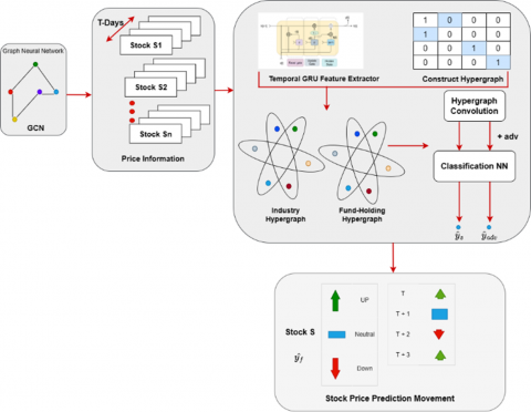
Figure 1. Proposed architecture combines historical stock data with hypergraph convolution graph to predict stock price movement
The price movement is dropping (-1), or stable (0) if the difference is higher than 0.50%. According to past research, these factors consider transaction costs like taxes to discover profitable trading opportunities [30]. The cross-entropy loss function predicts stock price changes.
$loss_{\text {hinge }}=-\sum_{c=0} C y_{o, c} \log \left(p_{o, c}\right)$
where, the authors take into account the projected likelihood of observation k, which is represented by the binary indicator y, which indicates whether or not the forecast of observation o is correctly classified. In addition, the authors have $\alpha$, which is the number of classes that stand at three in our particular scenario: growth, steady, and fall.
The class c is represented as o. When adversarial training is taken into account, the cumulative losses undergo a modification.
$loss_{total}=-\sum_{c=0} C y_{o, c} \log \left(p_{o, c}\right)-\beta \sum_{c=0} C y_{a, c} \log \left(p_{a, c}\right)$
The additive term denotes the adversarial loss, and the expected probability of accurately classifying a perturbed observation $o$ as the $c$ class is $p_{a c}$ - $\beta$ is a hyperparameter to encourage the model to categorize both the original objects and the disturbed data that governs the trade-off between the various sorts of loss. In Figure 1, the authors present a schematic representation of the framework that the authors have presented.
There are two models in the system:
Model A. The stock price is analysed using:
Model B employs a distinct approach in integrating industry data compared to model A. Model B employs a Gated Recurrent Unit (GRU) to capture the relationship between price and time, as opposed to a Graph Convolutional Network (GCN) used in previous studies. Model B incorporates adversarial samples into the classification layer instead of analyzing industrial data.
Merging the predictions from Models A and B, which comprise units a, b, c, d, e, and f, and a, c, d, e, f, and g, respectively, will result in an entirely novel representation, $\hat{y}_s$.
The predicted outcome of the adversarial situation by model B is denoted as $\hat{y}_{adv}$. The ultimate forecast, represented as $\hat{y}_f$, is determined by a voting process that takes into account both $\hat{y}_s$ and $\hat{y}_{adv}$.
Our suggested model differs from the current HGTAN in three ways [18]:
3.2 Adversarial training
The objective of adversarial training is to enhance the performance of models by incorporating hostile instances alongside clean data, so enabling them to reliably generate appropriate responses even in the face of harmful attacks. Because stock movements are unpredictable and changing, overfitting must be avoided to produce reliable projections. Addressing the current issue, Bai et al. [31] effectively validated the model's capacity to accurately mimic the unpredictability of stock attributes using adversarial training on financial time-series data. Feng et al. [32] recommended using a sentiment-guided generative adversarial network to solve the stock prediction problem. Zhang et al. [33] successfully achieved the next step of integrating adversarial training with transfer learning.
3.3 Hypergraph construction
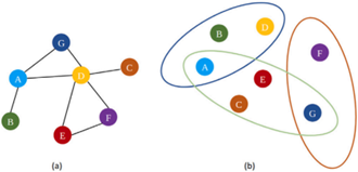
Definition 1 (Hypergraph). The notation $G=(V, E)$ can be used to represent an undirected hypergraph, The set of all nodes is represented by $V$ and all hyperedges are represented by $E$. Figure 2 demonstrates that hypergraphs allow for the representation of complex interactions between entities, as each edge $e$ can connect an endless number of vertices $v$. Nevertheless, as depicted in Figure 2, in elementary networks, a solitary edge has the capacity to exclusively link two vertices, so indicating a bilateral association between nodes. Hypergraphs are sometimes referred to as incidence matrices, which are represented as $H \in R^N X M$.
Figure 2. Graphs that are simple and hypergraphs
$h(\boldsymbol{i}, \boldsymbol{j})=\left\{\begin{array}{c}\mathbf{1}, f \text { node } i \text { is included in hyperedge } j \\ \mathbf{0}, \text { otherwise }\end{array}\right.$
Similar to study by Li et al. [34], the user's text is empty. To visually represent the relationships between industrial stocks and their corresponding ownership of capital, the authors create several hypergraphs. The industry hypergraph, like the fund-holding hypergraph, is distinguished by a solitary hyperedge that links all businesses within the same industry. Furthermore, every component in set V located at node v relies on 10 dimensions to determine their characteristics. To update the embeddings of each stock (node) and utilize them for price movement categorization, it is necessary to employ graph convolutions on the two hypergraphs.
3.4 GCN for industry information
For the purpose of generating an updated embedding for every trading day $t$, the authors utilize the daily stock prices $x_i^t$ of stock $s$ as stock features. This allows us to build an embedding that is up to date. Additionally, in order to improve the pairwise patterns of companies that are similar to one another, the authors add the appropriate industry information, denoted as $I_s$, into a generalized convolutional neural network, denoted as $f(\theta)$.
$x_i^t=f(\theta) \cdot x_s$
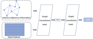
For the purpose of constructing undirected connections connecting stocks that belong to the same industry, the authors make use of two convolution layers and the data, as shown in Figure 3. For the purpose of processing the data relevant to the money, which would be taken into consideration at a later time, the authors abstained from employing GCN. In addition, the information regarding fund holdings is given less weight for a single stock when compared to the data on the industry. As per the findings of study by Jiang et al. [35], this phenomenon can be attributed to the fact that mutual funds are obligated to keep their portfolios diverse in order to comply to the diversification investing strategy. Data on money held, on the other hand, may provide insight into the direction in which the market is moving. After passing through the GCN layer, the time-series information will be acquired by transferring the new embedding, which is denoted by the symbol $x_i^t$.
Figure 3. Overview of GCN
3.5 Gated recurrent unit for long term dependency
In order to understand how the stock features are represented, a Gated Recurrent Unit (GRU) is utilised, as described in a prior investigation [36]. This is due to its capacity to detect dependencies in sequential data that span long periods of time. The input stock function has been enhanced by integrating industry impact. The GRU's primary purpose is to create a regulation system that regulates and alters data transmission between neural system cells. Several potential manifestations of this could include the following:
$\left\{\begin{array}{c}z=\sigma\left(W_z \cdot x_i^t+U_z \cdot h_{t-1}+b_z\right), \\ r=\sigma\left(W_r \cdot x_i^t+U_r \cdot h_{t-1}+b_r\right), \\ \hat{h}=\tanh \left(W_h \cdot x_i^t+r * U_h \cdot h_{t-1}+b_z\right) \\ h_t=z * h_{t-1}+(1-z) * \hat{h}\end{array}\right.$
In this equation, $x_i^t$ is given from Eq. (4), and $W_z, W_r, W_z$ the weight matrices are what ought to be trained. The hidden state, denoted as $h_{t-1}$, is composed of historical data originating from the previous trading day. Furthermore, instruction is necessary for the parameters $U_z, U_r, U_z$. The zgate functions as a reset gate, determining the extent to which prior information should be disregarded. In contrast, the r-gate acts as an update gate, determining the extent to which past knowledge should be transmitted to subsequent iterations. By utilising the update and reset gates, it may be possible to circumvent the vanishing gradient problem when backpropagating time series data. The currently under consideration information is denoted by the symbol "hath" within the framework of the current concealed state $h_t$ The temporal attention layer will be supplied with the newly constructed embedding $h_t$.
3.6 Ensemble learning
In the study by Chung et al. [37], the utilization of several ensemble approaches is recommended introduced two fundamental models, as depicted in Figure 1. (A) The GCN model will be utilized to analyze stock price and industry data. The resulting updated embeddings will then be inputted into a GRU model, which incorporates a temporal attention layer, hypergraph convolution network, and linear neural network for the purpose of prediction. (B) The stock features undergo a GRU, temporal attention layer, and hypergraph convolution network to produce a novel forecast. This forecast is subsequently combined with the prediction of model A, denoted as $\hat{y}_{\mathrm{s}}$, the linear prediction layer will receive adversarial examples obtained by hypergraph convolution, leading to the development of a $\hat{y}_{\text {adv }}$ model. Maximum voting is employed to allocate the sample to the classes that have received the highest number of votes, namely $\hat{y}_5$ and $\hat{y}_{\mathrm{adv}}$.
4.1 Experimental setup
The authors employ their dataset for data gathering to provide an equitable comparison with study by Qin et al. [38]. From April 1, 2013, to March 31, 2019, the Chinese A-share market had 758 shares for regular trading. The authors will validate technique by collecting data from other markets, such as the United States or Europe. In the dataset, each stock is represented by one of the six parameters that are listed below: the initial price, the closing price, the trading volume, the value, and the highest and lowest prices. After implementing the min-max normalization approach for each stock input feature independently, the results were displayed. In the case that trade data for specific shares is unavailable during the suspension period, the price attributes from the previous day will be applied regardless of the situation. According to the information provided by Bhola et al. [39], the dataset was segmented into three unique subsets: sixty percent was designated for training, twenty percent was designated for validation, and twenty percent was designated for testing. The hyperparameters of our model are going to be optimized through the use of fine-tuning, which is the purpose of the validation set. Securities are classified into 104 different categories according to Standard 3 of the Shenwan Industry Classification. The ‘fund-holding’ information had been taken from the quarterly reports of 61 A-share mutual funds that had been founded previous to the year 2013. Table 1 provides a comprehensive overview of the dataset's information in its entirety.
Table 1. Dataset summary
|
Data |
Numbers |
|
Nodes |
778 |
|
Attribute |
7 |
|
Industry-belonging relationship |
109 |
|
Fund-holding relationship |
63 |
|
Steady percentage |
25.12% |
|
Rising percentage |
39% |
|
Dropping percentage |
38.27% |
Baselines: The authors benchmark stock movement prediction findings against those of prior research, which includes five newly suggested graph neural network algorithms, one standard LSTM model, one multifaceted attention LSTM, and one trading strategy called mean reversion (MR).
Parameters: The authors run the specified ensemble learning framework using CUDA 10.2 and PyTorch 1.10.2. The authors tested the model using data from the latest 5, 10, and 20 trading days because the authors in the study [41] note that data longevity affects model performance. The authors employed hyperparameters tuned using study by Zhang et al. [41] validation set to level the playing field: For the temporal attention mechanism, $d_k$ and $d v$ are both eight, and stock has a feature dimension of 16, with a batch size of 32. Hidden GRU unit number 32. For the loss function 3, the study recommended setting $\beta$ as $1_{e-2}$ with a maximum of 600 epochs and a dropout rate of 0.5. Our baseline models are configured like their public counterparts.
Evaluation: The authors utilized the following metrics to evaluate the suggested model's classification effectiveness: accuracy, precision, recall, and F1 score. The metrics are computed as follows:
$\begin{gathered} Accuracy=\frac{T P+T N}{T P+T N+F P+F N} \\ Precision=\frac{T P}{T P+F P} \\ Recall=\frac{T P}{T P+F N}\end{gathered}$
The symbols TP and TN are used to denote the classes that have been positively predicted and the classes that have been negatively predicted, respectively. The mistakenly predicted positive classes are denoted by the symbol FP, whereas the incorrectly anticipated negative classes are denoted by the symbol FN. To compute the metric in the macro-setting, the authors make use of the scikit-learn module. At the same time, the authors perform multi-label classification, which involves three different movement directions. As an illustration, the formula for determining precision may be as follows:
$Precision =\left(\frac{T P_r}{T P_r+F P_r}+\frac{T P_s}{T P_s+F P_s}+\frac{T P_f}{T P_f+F P_f}\right) * \frac{1}{3}$
The acronyms r, s, and f represent the terms increase, steady, and decline, respectively.
4.2 Effectiveness results on the real-world dataset
The number of models that accurately predict the movement of stock prices on real-world benchmark datasets is presented in Tables 2-4. The look-back window for these models is the most recent five, ten, and twenty trading days. In terms of precision, recall, and F1 score, the suggested model beats the second-best baseline by increments of 1.14 percent, 3.63 percent, and 2.45 percent for three different trade periods. According to study by Li et al. [42], the F1 value takes into account precision and recall measurements, which helps to improve the sensitivity and generalizability of performance evaluation models. When it comes to investing in stocks, getting a high recall means making the most of every opportunity to generate money and also high precision. Therefore, it can be concluded that the F1 score is the most significant of these four parameters. The Wilcoxon signed rank test, a non-parametric used when the requirements for the t-test for two paired samples are not satisfied test, demonstrates that our model outperforms where (p>=0.5) the most advanced HGTAN, particularly in situations when sophisticated triple attention spanning hyperedges and hypergraphs is not utilized. Furthermore, our model improves the F1 score by 7.34 percent. Both hypergraph convolution and GCN are used to collect data on the movement of stock prices at the group level and pairwise, as demonstrated above. With data from the most recent 20 and 5 trading days, our model outperforms the competition, and it reaches its highest level of accuracy within a span of ten days.
Table 2. Results from comparing baselines and the suggested model for classification using data from five trading days
|
Method |
Accuracy |
Precision |
Recall |
F1-Score |
|
MR |
36.45% |
38.34% |
34.65% |
36.12% |
|
LSTM |
34.12% |
39.12% |
33.56% |
35.12% |
|
DARNN |
35.76% |
37.34% |
34.92% |
34.67% |
|
GCN+LSTM |
36.12% |
37.89% |
37.11% |
33.72% |
|
HATS |
37.44% |
38.37% |
35.68% |
35.89% |
|
TGC |
33.61% |
34.71% |
34.67% |
34.90% |
|
STHGCN |
38.11% |
39.45% |
35.12% |
36.12% |
|
HGTAN |
39.18% |
40.57% |
37.69% |
35.72% |
|
Proposed Method |
39.78% |
37.12% |
39.34% |
36.12% |
Table 3. Results from comparing baselines and the suggested model for classification using data from ten trading days
|
Method |
Accuracy |
Precision |
Recall |
F1-Score |
|
MR |
34.23% |
38.23% |
36.35% |
35.13% |
|
LSTM |
33.67% |
37.26% |
35.23% |
34.67% |
|
DARNN |
33.56% |
35.12% |
37.37% |
36.13% |
|
GCN+LSTM |
38.90% |
35.23% |
34.72% |
34.23% |
|
HATS |
35.83% |
35.89% |
33.45% |
37.90% |
|
TGC |
34.89% |
37.28% |
36.37% |
37.27% |
|
STHGCN |
35.27% |
34.68% |
35.98% |
33.58% |
|
HGTAN |
34.78% |
41.56% |
36.28% |
36.23% |
|
Proposed Method |
34.52% |
42.47% |
39.34% |
38.51% |
Table 4. Results from comparing baselines and the suggested model for classification using data from twenty trading days
|
Method |
Accuracy |
Precision |
Recall |
F1-Score |
|
MR |
32.89% |
38.19% |
36.12% |
36.34% |
|
LSTM |
33.00% |
39.46% |
37.33% |
39.45% |
|
DARNN |
33.02% |
40.12% |
32.80% |
38.24% |
|
GCN+LSTM |
33.09% |
41.03% |
34.82% |
39.34% |
|
HATS |
32.18% |
34.62% |
34.12% |
35.22% |
|
TGC |
33.17% |
33.12% |
36.32% |
38.23% |
|
STHGCN |
32.38% |
38.56% |
39.98% |
38.33% |
|
HGTAN |
32.68% |
41.23% |
40.28% |
39.21% |
|
Proposed Method |
33.23% |
41.48% |
39.34% |
40.11% |
4.3 Investment simulation and profitability
From April 23, 2019, to May 9, 2019, which is ten trading days, the authors compare our model to competitors using the same forecasting window size as study [42]. The findings are presented in Table 4. The constant prediction accuracy of the model, which reaches its highest point in five days, is one of its most significant advantages.
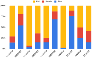
In seven days, it reaches an accuracy of more than 70 per cent (all accuracies more significant than 70 per cent are highlighted). The most advanced model, HGTAN, takes three days, and the rest of the models, for the most part, only take one of the ten trading days. Over ten trading days, four important market indices—the Hushen 300, the Shenzheng Zongzhi, the Shangzheng 50, and the Zhongxiao 300—entered what is known as a “bear market,” as seen in Figure 4. The Hushen 300, comprised of the 300 equities with the highest market capitalization and the most liquidity, witnessed a precipitous drop from 4019 on April 23, 2019, to 3599.7 on May 9, 2019, which caused investors to get concerned. In Figure 4, it is demonstrated that dropping stocks are prevalent for seven consecutive days (April 23, April 25, April 26, April 29, May 6, May 8, and May 9). Furthermore, our technique consistently achieves more than 70 per cent accuracy (except one day), demonstrating its effectiveness compared to other models and its capacity to avert loss.
Figure 4. Different movement of stocks
The authors analyze the profitability of multiple models from August 31, 2018 to October 31,2019, as presented in Table 4, according to the reference [42]. The cumulative return rate, called CR, is frequently used in profitability analysis (B14). The abbreviation SR refers to the Sharpe ratio, a quantitative measure that assesses the relationship between investment returns and associated risks.
$ Sharpe\,\, Ratio=\frac{E\left(R_s-R_f\right)}{\sigma_s}$
Within this particular framework, the symbols $E, R_s$, and $R_f$ represent the expected value, stock return, and risk-free rate, respectively. For instance, the interest rate on a one-year deposit in 2019 is $1.5 \%$. The standard deviation of the excess return on investments is also denoted by the symbol $\sigma_s$. Our approach is competitive in terms of risk management and has the maximum cumulative return rate at $22.33 \%$. In addition, its Sharpe ratio of 0.775 is the highest of any model the authors evaluated, indicating that it generates a greater profit under identical risk conditions. However, the main problem with the Sharpe ratio is that it can be accentuated by investments that don't have a normal distribution of returns.
4.4 Discussion and analysis
The authors evaluate the classification accuracy of the dataset by analyzing data from the past ten trading days. In Table 5, the authors evaluate the effectiveness of the second-best model, HGTAN, with that of our proposed framework and its components. This study demonstrates the enhancements made to each module, both on an individual basis and as a whole, through the implementation of our proposed architecture.
Table 5. An ablation study of proposed framework on dataset with 10 trading days as record
|
Method |
Accuracy |
Precision |
Recall |
F1-Score |
|
Module - A |
41.37 |
42.06 |
39.36 |
40.65 |
|
Module - B |
41.27 |
41.30 |
38.12 |
40.32 |
|
Module - C |
41.09 |
43.22 |
39.32 |
41.28 |
|
Module - D |
40.22 |
40.82 |
39.34 |
39.79 |
|
Module - E |
41.21 |
42.77 |
37.82 |
40.68 |
|
Module - F |
39.57 |
40.45 |
39.11 |
39.54 |
|
HGTAN |
39.83 |
42.72 |
38.90 |
40.12 |
|
Proposed Method |
40.41 |
41.20 |
39.41 |
40.49 |
The proposed framework prevails all versions in recall and F1 score because all modules improve performance relative to the baseline (Module D). The framework significantly outperforms HGTAN in accuracy, recall, and F1 score. Section 4.3 further notes that the proposed framework performs well during market downturns. When comparing modules, A and B, GCN improves F1 value by 0.33% and all four metrics by 2.28%. It's wrong to disregard pairwise relations because we've evaluated group-level data. GCN outperforms RNNs in price fluctuation learning. GCN will improve RNN model prediction by capturing industry-based stock volatility trends. Adversarial training with stock price stochasticity improves model resilience. Comparing modules B and C, C's accuracy, recall, and precision drop but F1 score increases. Hypergraph convolution enhances module D's accuracy by 2.31%, according to module B. Precision and F1 score can improve 2.17% and 1.02%. Comparing module F with the proposed framework demonstrates that hypergraphs are needed to predict stock prices using group-level data.
The prior work on stock movement prediction concentrated solely on historical price characteristics rather than group-wise and pairwise relations of important information. As a result, the study has weak generalizability due to the stochastic nature of stocks. When the GCN model is used first to capture patterns of stock volatility, the performance of the RNN model in terms of prediction is improved. Our findings lead us to the conclusion that RNN models should come after pairwise relation learning. An ensemble learning framework is the methodology that has been recommended as a solution to these challenges, which also helps investors improve their ability to predict market trends. Before RNN models, a graph convolution network quickly and effectively collects matched data that is specialized to a particular business. When the GRU paradigm and a temporal attention layer are utilized, hypergraph convolution networks are able to successfully acquire data from fund-holding groups and industries. Prior to the final prediction layer (B), adversarial training is implemented so as to simulate the unforeseeable movement that transpires throughout the training process. By employing ensemble learning, both models are capable of enhancing the interconnection and resilience of the learning process while retaining their individual merits. All the requisite components must be present in order to analyze the stock market through the utilization of data. By circumventing the need for intricate triple attention methods involving hyperedges and hypergraphs, our model outperforms the existing state of the art for the majority of indicators, especially in imperfect market environments. To ensure that our model is comparable to other models, the authors conducted tests in a single market and exclude COVID-19. Despite the fact that this limitation exists, the authors intend to test the strategy in more markets. Utilizing advanced deep learning techniques such as graph dynamic attention and graph contrastive learning; it is possible to employ these techniques for stock prediction tasks.
[1] Lee, C.Y., Soo, V.W. (2017). Predict stock price with financial news based on recurrent convolutional neural networks. In 2017 Conference on Technologies and Applications of Artificial Intelligence (TAAI), Taipei, Taiwan, pp. 160-165. https://doi.org/10.1109/TAAI.2017.27
[2] Singh, H. (2023). Prediction of Thyroid Disease using Deep Learning Techniques. In 2023 Second International Conference on Electrical, Electronics, Information and Communication Technologies (ICEEICT), Trichirappalli, India, pp. 1-7. https://doi.org/10.1109/ICEEICT56924.2023.10157812
[3] Hong, H., Torous, W., Valkanov, R. (2007). Do industries lead stock markets? Journal of Financial Economics, 83(2): 367-396, https://doi.org/10.1016/j.jfineco.2005.09.010
[4] Sawhney, R., Agarwal, S., Wadhwa, A., Shah, R.R. (2020). Spatiotemporal hypergraph convolution network for stock movement forecasting. In 2020 IEEE International Conference on Data Mining (ICDM), Sorrento, Italy, pp. 482-491. https://doi.org/10.1109/ICDM50108.2020.00057
[5] Cui, C., Li, X., Zhang, C., Guan, W., Wang, M. (2023). Temporal-relational hypergraph tri-attention networks for stock trend prediction. Pattern Recognition, 143: 109759. https://doi.org/10.1016/j.patcog.2023.109759
[6] Aghabozorgi, S., Teh, Y.W. (2014). Stock market co-movement assessment using a three-phase clustering method. Expert Systems with Applications, 41(4): 1301-1314. https://doi.org/10.1016/j.eswa.2013.08.028
[7] Berk, J.B., Van Binsbergen, J.H. (2015). Measuring skill in the mutual fund industry. Journal of Financial Economics, 118(1): 1-20. https://doi.org/10.1016/j.jfineco.2015.05.002
[8] Singh, H., Malhotra, M. (2023). Artificial intelligence based hybrid models for prediction of stock prices. In 2023 2nd International Conference for Innovation in Technology (INOCON), Bangalore, India, pp. 1-6. https://doi.org/10.1109/INOCON57975.2023.10101297
[9] Singh, H., Malhotra, M. (2024). Stock market and securities index prediction using artificial intelligence: A systematic review. Multidisciplinary Reviews, 7(4): 2024060-2024060. https://doi.org/10.31893/multirev.2024060
[10] Ye, J., Zhao, J., Ye, K., Xu, C. (2021). Multi-graph convolutional network for relationship-driven stock movement prediction. In 2020 25th International Conference on Pattern Recognition (ICPR), Milan, Italy, pp. 6702-6709. https://doi.org/10.1109/ICPR48806.2021.9412695
[11] Xiong, K., Ding, X., Du, L., Liu, T., Qin, B. (2021). Heterogeneous graph knowledge enhanced stock market prediction. AI Open, 2: 168-174. https://doi.org/10.1016/j.aiopen.2021.09.001
[12] Guo, L., Yin, H., Chen, T., Zhang, X., Zheng, K. (2021). Hierarchical hyperedge embedding-based representation learning for group recommendation. ACM Transactions on Information Systems (TOIS), 40(1): 1-27, https://doi.org/10.1145/3457949
[13] Singh, H., Sharma, C., Attri, V., & Singh, S. (2024). Time Series Forecast with Stock's Price Candlestick Patterns and Sequence Similarities. In 2024 International Conference on Emerging Smart Computing and Informatics (ESCI) (pp. 1-6). https://doi.org/10.1109/ESCI59607.2024.10497266
[14] Singh, H., Rani, A., Chugh, A., Singh, S. (2024). Utilising sentiment analysis to predict market movements in currency exchange rates. In 2024 3rd International Conference for Innovation in Technology (INOCON), Bangalore, India, 2024, pp. 1-7. https://doi.org/10.1109/INOCON60754.2024.10512061
[15] Singh, H., Malhotra, M. (2023). A Comparative Analysis of Share Price Prediction and Trend Direction Using Sentiment Analysis of Financial News Articles. In 2023 Global Conference on Information Technologies and Communications (GCITC), pp. 1-7. https://doi.org/10.1109/GCITC60406.2023.10426337
[16] Kaur, M., Joshi, K., Singh, H. (2022). An efficient approach for sentiment analysis using data mining algorithms. In 2022 International Conference on Computing, Communication and Power Technology (IC3P), Visakhapatnam, India, pp. 81-87. https://doi.org/10.1109/IC3P52835.2022.00025
[17] Singh, H., Shukla, A.K. (2021). An analysis of Indian election outcomes using machine learning. In 2021 10th International Conference on System Modeling & Advancement in Research Trends (SMART), Moradabad, India, pp. 297-306. https://doi.org/10.1109/SMART52563.2021.9676303
[18] Shukla, A.K., Singh, H. (2019). Your OTP is also not secure: Security issues of mobile apps in the E-commerce. International Journal of Engineering and Advanced Technology (IJEAT), 9(1): 3225-3228. https://doi.org/10.35940/ijeat.F9264.109119
[19] Shukla, A.K. (2021). Analysis of stock market prediction models using deep learning. Bioscience Biotechnology Research Communications, 14(9): 74-80. https://doi.org/10.21786/bbrc/14.9.17
[20] Singh, H., Malhotra, M. (2023). A novel approach of stock price direction and price prediction based on investor’s sentiments. SN Computer Science, 4(6): 823. https://doi.org/10.1007/s42979-023-02349-0
[21] Gaba, S., Gupta, M., Singh, H. (2023). A comprehensive survey on VANET security attacks. In AIP Conference Proceedings, Mohali, India, p. 020029. https://doi.org/10.1063/5.0145236
[22] Singh, H., Malhotra, M. (2023). A time series analysis-based stock price prediction framework using artificial intelligence. In International Conference on Artificial Intelligence of Things, Switzerland, pp. 280-289. https://doi.org/10.1007/978-3-031-48781-1_22
[23] Chawla, J., Walia, N.K. (2022). Artificial intelligence-based techniques in respiratory healthcare services: A review. In 2022 3rd International Conference on Computing, Analytics and Networks (ICAN), Rajpura, Punjab, India, pp. 1-4. https://doi.org/10.1109/ICAN56228.2022.10007236
[24] Jaswal, G.S., Sasan, T.K., Kaur, J. (2023). Early-stage emphysema detection in chest x-ray images: A Machine learning based approach. In 2023 World Conference on Communication & Computing (WCONF), Raipur, India, pp. 1-6. https://doi.org/10.1109/WCONF58270.2023.10235244
[25] Baghel, Y., Jindal, H., Chawla, J. (2023). Early diagnosis of emphysema using convolutional neural networks. In 2023 World Conference on Communication & Computing (WCONF), Raipur, India, pp. 1-5. https://doi.org/10.1109/WCONF58270.2023.10235036
[26] Singh, H., Malhotra, M. (2023). A novel approach for predict stock prices in fusion of investor's sentiment and stock data. In 2023 3rd International Conference on Technological Advancements in Computational Sciences (ICTACS), Tashkent, Uzbekistan, pp. 1163-1169. https://doi.org/10.1109/ICTACS59847.2023.10389912
[27] Chen, Y., Wei, Z., Huang, X. (2018). Incorporating corporation relationship via graph convolutional neural networks for stock price prediction. In Proceedings of the 27th ACM International Conference on Information and Knowledge Management, Torino, Italy, pp. 1655-1658. https://doi.org/10.1145/3269206.3269269
[28] Ye, J., Zhao, J., Ye, K., Xu, C. (2021). Multi-graph convolutional network for relationship-driven stock movement prediction. In 2020 25th International Conference on Pattern Recognition (ICPR), Milan, Italy, pp. 6702-6709. https://doi.org/10.1109/ICPR48806.2021.9412695
[29] Xiong, K., Ding, X., Du, L., Liu, T., Qin, B. (2021). Heterogeneous graph knowledge enhanced stock market prediction. AI Open, 2: 168-174. https://doi.org/10.1016/j.aiopen.2021.09.001
[30] Guo, L., Yin, H., Chen, T., Zhang, X., Zheng, K. (2021). Hierarchical hyperedge embedding-based representation learning for group recommendation. ACM Transactions on Information Systems (TOIS), 40(1): 1-27, https://doi.org/10.1145/3457949
[31] Bai, T., Luo, J., Zhao, J., Wen, B., Wang, Q. (2021). Recent advances in adversarial training for adversarial robustness. arXiv Preprint arXiv:2102.01356. https://doi.org/10.48550/arXiv.2102.01356
[32] Feng, F., He, X., Wang, X., Luo, C., Liu, Y., Chua, T.S. (2019). Temporal relational ranking for stock prediction. ACM Transactions on Information Systems (TOIS), 37(2): 1-30. https://doi.org/10.1145/3309547
[33] Zhang, Y., Li, J., Wang, H., Choi, S.C.T. (2021). Sentiment-guided adversarial learning for stock price prediction. Frontiers in Applied Mathematics and Statistics, 7: 601105. https://doi.org/10.3389/fams.2021.601105
[34] Li, M., Zhang, Y., Li, X., Cai, L., Yin, B. (2022). Multi-view hypergraph neural networks for student academic performance prediction. Engineering Applications of Artificial Intelligence, 114: 105174. https://doi.org/10.1016/j.engappai.2022.105174
[35] Jiang, M., Liu, J., Zhang, L., Liu, C. (2020). An improved Stacking framework for stock index prediction by leveraging tree-based ensemble models and deep learning algorithms. Physica A: Statistical Mechanics and its Applications, 541: 122272. https://doi.org/10.1016/j.physa.2019.122272
[36] Zhao, Y., Li, J., Yu, L. (2017). A deep learning ensemble approach for crude oil price forecasting. Energy Economics, 66: 9-16. https://doi.org/10.1016/j.eneco.2017.05.023
[37] Chung, J., Gulcehre, C., Cho, K., Bengio, Y. (2014). Empirical evaluation of gated recurrent neural networks on sequence modeling. arXiv Preprint arXiv:1412.3555. https://doi.org/10.48550/arXiv.1412.3555
[38] Qin, Y., Song, D., Chen, H., Cheng, W., Jiang, G., Cottrell, G. (2017). A dual-stage attention-based recurrent neural network for time series prediction. arXiv Preprint arXiv:1704.02971. https://doi.org/10.48550/arXiv.1704.02971
[39] Bhola, J., Shabaz, M., Dhiman, G., Vimal, S., Subbulakshmi, P., Soni, S.K. (2022). Performance evaluation of multilayer clustering network using distributed energy efficient clustering with enhanced threshold protocol. Wireless Personal Communications, 126(3): 2175-2189. https://doi.org/10.1007/s11277-021-08780-x
[40] Feng, F., Chen, H., He, X., Ding, J., Sun, M., Chua, T.S. (2019). Enhancing stock movement prediction with adversarial training. Proceedings of the Twenty-Eighth International Joint Conference on Artificial Intelligence (IJCAI-19), China, pp. 5843-5849. https://doi.org/10.48550/arXiv.1810.09936
[41] Zhang, Y., Li, J., Wang, H., Choi, S.C.T. (2021). Sentiment-guided adversarial learning for stock price prediction. Frontiers in Applied Mathematics and Statistics, 7: 601105. https://doi.org/10.3389/fams.2021.601105
[42] Li, Y., Dai, H.N., Zheng, Z. (2022). Selective transfer learning with adversarial training for stock movement prediction. Connection Science, 34(1): 492-510. https://doi.org/10.1080/09540091.2021.2021143