Sana Hamiane*![]() | Youssef Ghanou
| Youssef Ghanou![]() | Hamid Khalifi
| Hamid Khalifi![]() | Meryam Telmem
| Meryam Telmem![]()
© 2024 The authors. This article is published by IIETA and is licensed under the CC BY 4.0 license (http://creativecommons.org/licenses/by/4.0/).
OPEN ACCESS
Gross domestic product (GDP) is an effective indicator of economic development, and GDP forecasts provide a better understanding of future economic trends. This article investigates three methods of forecasting GDP: LSTM, ARIMA and a hybrid approach that combines two models. The principal aim is to compare the performance of these methods by computing mean square error (MSE), Root Mean Square Error (RMSE), Mean Average Error (MAE), the coefficient of determination (R2) and to determine which model provides the most accurate and reliable forecasts. The study collected quarterly GDP data from the Federal Reserve Economic Data, covering a period of 75 years from 1947 to 2022. The LSTM model, using the HE initialization technique to initialize the weights, was trained and tested using the GDP data. the ARIMA model was configured with parameters (1,2,1), and the hybrid (ARIMA-LSTM) model combined the strengths of both approaches. It was found that LSTM (MSE=0.010, RMSE=0.104, MAE=0.077, R2=0.96), ARIMA (MSE=0.095, RMSE=0.309, MAE=0.286, R2=0.75) and Hybrid (MSE=0.0018, RMSE=0.043, MAE=0.028, R2=0.99) and the hybrid model achieves better prediction accuracy than the individual models in predicting GDP.
Long Short-Term Memory (LSTM), economic and financial time series data, gross domestique product, GDP, Autoregressive Integrated Moving Average (ARIMA), hybrid models, He initialization
Forecasting time series accurately is a critical challenge with significant implications, especially in predicting economic growth. Gross Domestic Product (GDP) is one of the most important economic indicators for comparing and evaluating the economic performance of countries and regions, and economists are constantly in search of better ways to predict GDP [1, 2].
Gross Domestic Product (GDP), a comprehensive indicator, is determined through various macroeconomic measures. These indicators several multiple areas, including rural development, economy and growth, education, energy and mining, environment, financial sector, public and private sectors, and technology. The collective dynamics of these indicators significantly influence the overall performance and fluctuations in GDP [3].
Accurately forecasting GDP is a major challenge due to the complexity of these economic factors. Traditional forecasting techniques such as ARIMA, SARIMA, and ARMA have seen extensive use in predicting GDP time series [4, 5]. However, these methods face limitations and might not be well-suited for non-linear data or time series characterized by complex trends and seasonality.
In recent years, the field of predictive modeling has been transformed by machine learning, particularly through the advancements in deep learning algorithms. These methods have enabled a novel way of understanding the interactions between variables by employing a sophisticated, multi-layered structural approach [6]. Among these, machine learning techniques like Support Vector Machines (SVM) and Random Forests (RF), as well as deep learning algorithms including Recurrent Neural Networks (RNN) and Long Short-Term Memory (LSTM) networks, have drawn significant interest. These techniques are widely applied across different fields, especially in finance [7-9]. Deep learning methods excel at recognizing the structure and patterns in data [10], including non-linearity and complexity, particularly within the context of time series forecasting. In particular, the LSTM architecture, developed in 1997 by Hochreiter and Schmidhuber [11], offers a more fitting solution. This architecture, an extension of the recurrent neural network (RNN), is capable of handling the temporal nature of sequential data. LSTMs excel at capturing long-term dependencies and non-linear relationships in time series data [12-16], making them powerful tools for forecasting GDP time series.
This article investigates whether hybrid models can outperform traditional forecasting methods for GDP time series data. It will model GDP data and examine three methods. The first approach is a connectionist method using a Long Short-Term Memory (LSTM) network, which is capable of self-learning and capturing long-term dependencies. The second method is a statistical approach, employing an Autoregressive Integrated Moving Average (ARIMA) process, based on the Box and Jenkins methodology, recognized for its effectiveness in modeling time series dependencies. Finally, we will examine a hybrid ARIMA-LSTM model that combines the strengths of both approaches.
The novelty of our work lies in the proposal of a hybrid approach to GDP forecasting, an approach not employed in the existing literature. This approach combines the seasonal decomposition method for time series analysis, thus combining the strengths of statistical techniques and neural networks. Our study focuses on prediction from the quarterly GDP dataset, with the aim of evaluating the performance of three distinct approaches: LSTM, ARIMA and the hybrid model.
The organization of this article is as follows: Section two contains a review of the literature on GDP time series forecasting methods, touching on traditional, machine learning, and hybrid approaches. Section three dives into the specifics of LSTM and ARIMA models and their implementation in time series forecasting. Section four provides details on the dataset used and the methodology for evaluating the accuracy of the LSTM, ARIMA, and hybrid models. The results of the three models are presented in section five. In section six, there's a discussion on the findings, including a comparison of the models' performances against some previous works. The conclusion highlights the primary insights of the study.
This section offers a comprehensive review of contemporary and pertinent studies in the domain of GDP time series forecasting.
Rigopoulos [17] explored the application of the LSTM model for forecasting Greece's GDP. Findings indicated the LSTM approach's superiority in predicting stationary series, its competitive performance against the ARIMA model, and its advantage over the k-NN method.
Lai [18] assessed three neural network models, namely bat algorithm-LSTM, PSO-Elman NN, and genetic algorithm-backpropagation neural network, using Sichuan's GDP data from 1992 to 2020. The PSO-Elman NN model emerged as the top performer in GDP forecasting.
Dritsaki [19] utilized an ARIMA (1,1,1) model with data from 1980 to 2013 to predict Greece's real GDP rate for 2015 to 2017, revealing a consistent upward trend in the real GDP rate.
In the study by Sa'adah and Wibowo [20], LSTM and RNN models were employed to predict GDP growth during the Covid-19 pandemic. By integrating the tanh activation function into LSTM2 and RNN2, predictive accuracy surged from 80% to 90%.
In the study by Urrutia et al. [21], a comparative analysis assessed GDP forecasts for the Philippines, employing both ARIMA and Bayesian Artificial Neural Networks. The findings highlighted the superior predictive capability of the Bayesian Artificial Neural Network over the ARIMA method in forecasting the Philippines' GDP.
Sunitha et al. [22] Presented two forecasting methods for estimating India's annual global GDP: one based on ARIMA and the other on three types of artificial neural networks (FFNN, RNN, and RBF). The findings revealed that the ANN method, specifically the RBF Network, yielded superior forecasts.
Presented the application of the Nonlinear Autoregressive [23] with Variables (NARX) model to forecast time series in Italy, achieving a notable mean squared error (MSE) of 0.079 and a high accuracy rate of 0.87.
In recent times, researchers have progressively focused on integrating multiple data sources into hybrid models to enhance the precision of GDP forecasting. For example, Demir et al. [24] utilized an artificial neural network (ANN) model to predict Japan's GDP growth. The study compared the efficacy of multiple regression models against a hybrid approach that combines ANN with multiple regression models. The findings indicated that the hybrid model outperforms multiple regression models in terms of accuracy.
In the study by Hua [25], used the ARIMA and BPNN models to create a GDP forecasting model for the province of H. The results showed that the ARIMA model had a better long-term predictive effect than the improved combined model, and that the combined model outperformed a short-term prediction.
Ngige [26] proposed a multi-layer neural network that combined the ARIMA model with a feed-forward artificial neural network for predicting Kenya's GDP. These multi-layer models demonstrated strong performance in GDP prediction.
In the study by Lu [27], a novel approach combining the backpropagation neural network with the ARIMA model was proposed, leading to a unified model capable of accurately forecasting the daily price of the nonlinear residual of GDP.
In the field of economics, ARIMA and LSTM models offer powerful frameworks for the analysis and forecasting of time series data in economics. By capturing the intricate dynamics of economic variables, these models facilitate the prediction of trends and patterns, contributing significantly to economic analysis and decision-making processes. A brief background on ARIMA and LSTM will be presented in this section.
3.1 ARIMA
The ARIMA (Autoregressive Integrated Moving Average) model is primarily used for forecasting a single time series variable by encapsulating it within a framework that integrates autoregressive (AR) and moving average (MA) processes [28]. The foundational equation for the AR component is illustrated below:
$x(t)=i=1 \sum p \alpha i x(t-i)$ (1)
where, t is the time step, x(t) the predicted value, p the number of AR terms, and α the AR coefficients. The moving average (MA) part is:
$x(t)=i=1 \sum q \beta i \epsilon(t-i)$ (2)
with q as the MA terms count, β the MA coefficients, and ϵ the error term. Integrating both, the ARIMA model can be expressed as:
$x(t)=i=1 \sum p \alpha i x(t-i)+i=1 \sum q \beta i \epsilon(t-i)$ (3)
3.2 LSTM
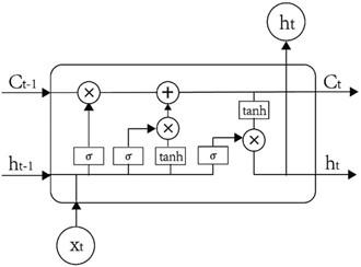
LSTMs, represent an advanced variant of Recurrent Neural Networks (RNNs), engineered specifically to address the issue of vanishing gradients, a significant limitation identified in conventional RNNs by Hochreiter and Schmidhuber [29] in 1997. By incorporating a system of gates, LSTMs can smartly decide which information to keep and which to let go, allowing them to remember important data over long periods without losing track due to the vanishing gradient problem. This gate system includes three key components: an input gate to add information to the memory cell, a forget gate to remove unneeded data, and an output gate to control the flow to the next network layer [22]. This setup makes LSTMs particularly adept at forecasting and analyzing sequences with long-term dependencies, outperforming traditional RNNs that struggle with these tasks. The LSTM cell, as depicted in Figure 1.
Figure 1. The LSTM cell, as conceptualized by Hochreiter and Schmidhuber in 1997 [30]
In an LSTM model, input data and previous output are processed at each time step. The model's hidden output, ht, is calculated using specific equations for the forget gate (Ft), input gate (It), and output gate (Ot). These components control the flow of information, allowing LSTMs to retain relevant data over time and address issues like vanishing gradients.
$F t=\sigma\left(w_f x_t+w_{h f} h_{t-1}+b_f\right)$ (4)
$I t=\sigma\left(w_i x_t+w_{h i} h_{t-1}+b_i\right)$ (5)
$O t=\sigma\left(w_o x_t+w_{h o} h_{t-1}+b_O\right)$ (6)
$c t=F_f c_{t-1}+I_t \tanh \left(w_c x_t+w_{h c} h_{t-1}+b_c\right)$ (7)
$h t=O_t \tanh \left(c_t\right)$ (8)
In the equations, σ denotes the sigmoid activation function, w terms stand for the weight matrices, and b signifies the biases in the model. Here, ht−1 is the output from the previous step, xt is the present input, ct−1 represents the previous memory cell's state, and ct indicates the current memory cell's state. These elements are crucial for calculating the LSTM model's operations, facilitating the management and update of information over time.
Long Short-Term Memory (LSTM) neural networks are extensively applied across a variety of fields, chiefly for their adeptness in managing sequential or temporal data. These networks are particularly valued for their capability to retain information over long periods, thus adeptly surmounting issues such as gradient vanishing or saturation, which are prevalent in traditional recurrent neural networks (RNNs) [31]. In our research, aiming to boost the LSTM model's efficacy in predicting GDP, we adopted the He initialization method. This approach is especially apt for LSTM models that employ the Rectified Linear Unit (ReLU) activation function, especially relevant in the analysis of time series data. The application of He initialization [32] has been instrumental in averting neuron saturation, culminating in marked enhancements in the model's forecasting accuracy for GDP.
This section of the study provides a detailed analysis of the ARIMA and LSTM models employed for prediction purposes. It investigates the fundamental principles and modeling procedures involved in creating the hybrid model, which is a combination of the ARIMA and LSTM models.
4.1 ARIMA and LSTM
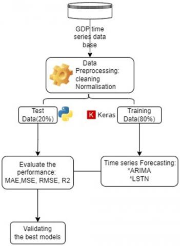
The proposed methodology in this study is divided into two distinct structures. In the first structure, we utilize a Long Short-Term Memory (LSTM) model and an Autoregressive Integrated Moving Average (ARIMA) model. In the LSTM model, a single hidden layer architecture with 16 neurons is utilized to retain internal network information. On the other hand, for the ARIMA model, different orders of differentiation were applied to ensure the data is stationary. The first structure, as depicted in Figure 2, incorporates these components.
Figure 2. Structure1 adopted for GDP prediction
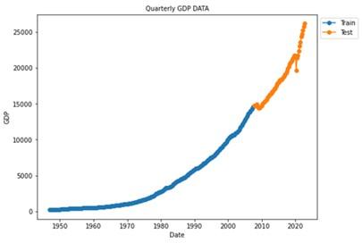
Data Preprocessing: is a crucial series of steps designed to optimally prepare a dataset for modeling. In this context, we focus on US quarterly GDP data covering the period from 1947 to 2022, as sourced from the Federal Reserve Economic Data [33]. The dataset is partitioned into two segments: the first, spanning from January 1, 1947, to July 1, 2007, is earmarked for training the model; the second, ranging from October 1, 2007, to October 1, 2022, is reserved for testing purposes.
The selection of a 75-year dataset for analyzing economic indicators like GDP is driven by the desire to comprehensively understand economic cycles, trends, and behaviors over time, encompassing expansion, recession, and recovery phases. the extensive dataset supports statistical and deep learning analyses to detect patterns and predict future trends, while also facilitating the study of long-term effects not visible in shorter datasets.
The preprocessing phase starts with normalization and cleaning to enhance data quality. For normalization, the scikit-learn StandardScaler method is employed to standardize the dataset. Cleaning involves the removal of missing values and outliers, in addition to applying feature scaling. These steps ensure that the data conforms to a uniform format, significantly boosting the model's ability to learn effectively.
The model was developed using Python and the Keras libraries, which provide extensive functionalities for building and training neural networks and machine learning models.
Figure 3. Structure 2 adopted for GDP prediction
Time series Forecasting GDP with two model ARIMA and LSTM.
Validating the best models: In this study, the performance of the models was evaluated based on some quantitative statistics such as mean square error (MSE), Mean Absolute Error (MAE), Root Mean Squared Error (RMSE), and coefficient of determination $\left(R^2\right)$.
$\mathrm{MSE}=\sum_{i=1}^n \frac{\left(y_i-y_{\text {pred }, i}\right)^2}{n}$ (9)
$\mathrm{RMSE}=\sqrt{\sum_{i=1}^n \frac{\left(y_i-y_{\text {pred }, i}\right)^2}{n}}$ (10)
$\mathrm{MAE}=\sum_{i=1}^n \frac{\left|y_i-y_{\text {pred }, i}\right|}{n}$ (11)
$\mathrm{R} 2=\frac{\sum_{i=1}^n\left(y_{\text {pred }, i}-y_{\text {pred }, \text { mean }}\right)^2}{\sum_{i=1}^n\left(y_i-y_{\text {mean }}\right)^2}$ (12)
where, "n" denotes the number of data points utilized for estimation, "$y_i$" represents the actual value of the i-th element within the dataset and "$y_{p r e d, i}$" signifies the predicted value of the i-th element within the dataset.
The process of validating the models involves comparing the predicted data with the actual test data. This is done by splitting the dataset into a training set and a test set to evaluate the predictive ability of the models.
4.2 Hybrid models
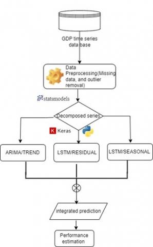
In the second structure, using the same quarterly GDP data and the same configuration of ARIMA and LSTM models, the hybrid model takes a completely different approach in terms of data preparation. The data set is split into three separate sections. The time series data can be divided into trend, seasonal, and residual categories using the seasonal decomposition tool found in the statsmodels package. The trend component is subject to the ARIMA model, whilst the seasonal component and residual component are both subject to the LSTM model. Combining the forecasts from each component yields the final prediction result, which provides a more precise and thorough projection of GDP. The second building is seen in Figure 3.
The LSTN and ARIMA models underwent training with US quarterly GDP data covering the period from 1947 to 2022, acquired from the Federal Reserve Economic Data. Table 1 illustrates examples of the dataset used. The primary aim was to utilize historical data for forecasting future quarterly GDP values.
Table 1. GDP Data of US [33]
|
Year |
GDP Values |
|
1/1/1947 |
243.164 |
|
4/1/1947 |
245.968 |
|
7/1/1947 |
249.585 |
|
10/1/1947 |
259.745 |
|
⁝ |
⁝ |
|
7/1/2022 |
25723.941 |
|
10/1/2022 |
26144.956 |
5.1 Arima model result
Stationarity testing was conducted on the GDP time series. Initial examination of the data involved time plots, depicted in Figure 4, which visually illustrate the non-stationary nature of the US GDP series.
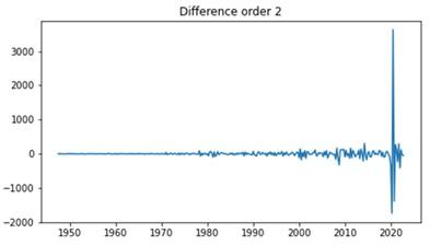
Two differences were taken to eliminate any seasonality and trend in the data. Subsequently, the augmented Dickey-Fuller test was applied to the differenced time series, revealing a p-value of 0.00. This result, as depicted in Figure 5, confirms the attainment of stationarity in the series.
Figure 6 presents the Autocorrelation Function (ACF) and Partial Autocorrelation Function (PACF) plots for the GDP time series. The ACF coefficients signify the correlation between the time series and its various lags, while the PACF coefficients provide insights into the partial correlations relevant for ARIMA model identification. The selection of the most suitable model will be determined based on the criteria of minimizing the Bayesian Information Criterion (BIC) and the Akaike Information Criterion (AIC) values. The results of this model comparison and selection process will be presented in the following Table 2.
Figure 4. Plot for US GDP data
Figure 5. Time series plot of quarterly GDP -at second difference
Figure 6. ACF and PACF plot for the time series of the Quarterly GDP
Table 2. The AIC and BIC values for tentative ARIMA
|
Box-Jenkins Model |
AIC Value |
BIC Value |
|
ARIMA (0,2,0) |
4204.85 |
4208.56 |
|
ARIMA (0,2,1) |
3981.13 |
3988.55 |
|
ARIMA (0,2,2) |
3978.30 |
3989.43 |
|
ARIMA (1,2,0) |
4075.60 |
4083.02 |
|
ARIMA (1,2,1) |
3977.51 |
3988.64 |
|
ARIMA (1,2,2) |
3979.10 |
3993.94 |
|
ARIMA (2,2,0) |
4031.17 |
4042.30 |
|
ARIMA (2,2,1) |
3978.59 |
3993.43 |
|
ARIMA (2,2,2 |
3978.09 |
3996.64 |
Based on the results presented in the Table 2 above, it is evident that the ARIMA (1,2,1) model is the optimal choice, as it exhibits the lowest AIC and BIC values. Therefore, the ARIMA (1,2,1) model is selected for the purpose of forecasting future values in this study. Depending on the ARIMA model, model fitting is performed on the quarterly GDP data, and the results of the error estimation studies are presented in Table 3. To improve the accuracy of the ARIMA model's predictions, we will investigate optimization strategies involving the combination of different models.
Table 3. Validation metrics of the ARIMA mode
|
MSE |
RMSE |
MAE |
R2 |
|
0.095 |
0.309 |
0.286 |
0.75 |
5.2 LSTM model result
In this phase of the study, we utilized a Long Short-Term Memory (LSTM) architecture based on time series GDP data, the model utilized the HE initialization technique to initialize the weights and Earlystopping regularization to prevent overfitting [34], The model incorporated GDP data from the preceding three quarters as input, with the GDP value of the current quarter serving as the target output. This sequential approach was consistently applied across the dataset, as outlined in Table 4. Subsequently, the model's performance was evaluated on a test set comprising 20% of the total dataset. Additionally, Table 5 presents the configuration parameters for the LSTM models developed in this study, providing insights into the model setup and optimization choices.
Table 4. Sequence dataset
|
Input |
Output |
|
1947(01-04-07) GDP |
1947(10) GDP |
|
1997(04-07-10) GDP |
1948(01) GDP |
|
… |
… |
|
2022(01-04-07) GDP |
2022(10) GDP |
Table 5. LSTM learning parameters
|
Parameter Name |
Value |
|
Number of layers, Neurons |
(1,3), (2,16), (3,1) |
|
learning_rate |
0.001 |
|
Batch_size |
32 |
|
Epoch |
100 |
|
Training function |
[Relu, linear] |
|
Performance function |
MSE |
|
Weight initializer |
HE initialization |
|
optimizer |
Adam |
|
Sequence lenght |
3 Quartly |
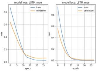
Training of the model was conducted using historical data spanning from 1947 to 2007, while validation of the model was performed on separate validation data spanning from 2007 to 2022, as illustrated in Figure 7. The LSTM network prediction is based on the principle of regression. This means that a predicted value at a given time (t) is the result of learning from all previous values up to time (t-1).
Figure 7. The learning process of LSTM model
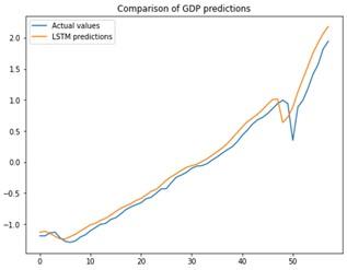
The LSTM model demonstrated high accuracy in forecasting quarterly GDP values, achieving minimal error metrics on the test set with MSE=0.010, MAE=0.077, and RMSE=0.104. Its predictions closely aligned with actual GDP figures, as shown in Figure 8, underscoring its effectiveness and reliability in economic forecasting.
To evaluate the model's predictive capability, we calculated the coefficient of determination (R2). The R2 value quantifies the proportion of variance in the data that is accounted for by the model, was found to be 0.96. This indicates that our LSTM model accurately accounted for 96% of the variance in the quarterly GDP data, signifying that our predictions were remarkably precise and dependable.
Figure 8. Actual vs. predicted LSTM
5.3 Hybrid model result
The parameters utilized in the hybrid model were the same as those in the LSTM and ARIMA models that came before it. The components of trends, seasonality, and residual data from the time series dataset were separated. Using the seasonal decompose function offered by the statsmodels package, this decomposition was carried out. Then, instruction was given to each of these parts.
Figure 9. Actual vs. predicted hybrid
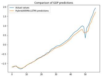
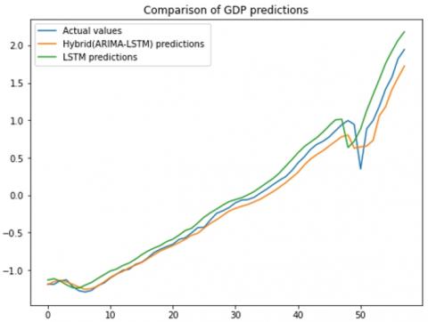
The combined predictions from each component are shown in Figure 9 as the final prediction result, the hybrid model, combining LSTM and ARIMA (1,2,1), produced highly accurate predictions as depicted in Figure 10, closely tracking the movement of the dataset. The hybrid model achieved a significantly lower error rate, measured by MSE=0.0018, MAE= 0.028 and RMSE=0.043. Furthermore, the coefficient of determination (R2) was found to be 0.99.
Figure 10. Actual vs. predicted
We compared of the proposed hybrid model against individual models, focusing on their performance in forecasting gross domestic product (GDP) on a quarterly basis using a basic univariate dataset. The highlights of this comparison is presented in Figure 10, which illustrates the GDP forecasts made by the hybrid models versus those generated from the basic data set. In addition, Table 6 shows the valuation parameters used to facilitate a more detailed comparison between the different modeling approaches.
The ARIMA (1,2,1) model, with its predictive ability (R2 of 0.75), demonstrates the effectiveness of linear models in capturing trends and seasonality in economic data sets. However, its relatively higher MSE, MAE and MSE highlight a critical limitation, the difficulty of dealing with non-linear relationships and volatile economic patterns, which are often present in GDP data.
The LSTM model marks a significant advance in forecast accuracy, as indicated by its superior R2 value of 0.96. The strength of this model lies in its ability to model complex, non-linear interactions and long-term dependencies in the data. However, this advanced capability comes with the risk of increased computational complexity and over-fitting, underlining the importance of careful model tuning and validation.
The hybrid ARIMA-LSTM model emerge as standout performers in our study, with a near-perfect R2 of 0.99. This model combines the linear trend analysis power of ARIMA with the pattern recognition capabilities of LSTM, offering a robust solution that efficiently handles both linear and non-linear data features. However, it requires more sophisticated data preprocessing and parameter tuning and demands more Figure 10. Actual vs. predicted LSTM processing power and time for training and optimization.
Table 6. Final predictions results
|
Model |
MSE |
MAE |
RMSE |
R2 |
|
ARIMA (1,2,1) |
0.095 |
0.286 |
0.309 |
0.75 |
|
LSTM |
0.010 |
0.077 |
0.104 |
0.96 |
|
Hybrid (ARIMA (1,2,1)-LSTM) |
0.0018 |
0.028 |
0.043 |
0.99 |
6.1 Validate the proposed approach with some previous studies
Comparison between the proposed approach and other scientific papers, such as those documented by Muchisha et al. [8, 20, 25, 23], reveals a broad application of machine-learning techniques and deep learning for GDP prediction. These studies reported accuracies of 91%, 80-90%, 98.71%, and 87%, respectively. Table 7 provides a comparative analysis of model accuracies, highlighting the performance of the proposed approach relative to existing methods.
Table 7. Comparison of the proposed work with the existing works in the literature
|
Work |
Technique |
Dataset |
Accuracy |
|
[8] |
lasso regression |
Quarterly GDP |
91% |
|
[20] |
LSTM, RNN |
Annual GDP |
80-90% |
|
[25] |
Hybrid (ARIMA and BPNN) |
Annual GDP |
98.71% |
|
[23] |
Nonlinear Autoregressive with Exogenous Variables (NARX) |
Annual GDP |
87% |
|
Proposed Approach |
Hybrid (LSTM-ARIMA) |
Quarterly GDP |
99% |
The proposed approach enhances prediction accuracy by 8% over Lasso regression, demonstrates a 12% improvement in classification accuracy compared to the Nonlinear Autoregressive with Exogenous Variables (NARX) model, and registers a marginal increase of 0.29% over the Hybrid (ARIMA and BPNN) model. Moreover, it surpasses the LSTM-RNN model by 9% in classification accuracy. These findings underscore the proposed method's superior performance, establishing it as the most accurate among the reviewed forecasting models.
This article conducts a comparative analysis of three forecasting models LSTM, ARIMA, and a hybrid LSTM-ARIMA model for predicting quarterly GDP. The results highlight the superior performance of the hybrid model in forecasting quarterly GDP, surpassing both the traditional ARIMA and LSTM models and exceeding previously reported outcomes in the literature.
The results of our study show that the hybrid model achieves higher predictive accuracy than both the LSTM and ARIMA models, with impressive metrics such as an MSE of 0.0018, an MAE of 0.028, and an RMSE of 0.043, along with an exceptional fit of approximately 99%. These outcomes establish the hybrid model as the superior choice for quarterly GDP prediction, as it effectively captures the complex and nonlinear relationships within time series data. The insights from our study can aid policymakers in devising more precise long-term economic policies. Additionally, hybrid models, as evidenced in this research and prior studies, typically exhibit significant predictive power. However, it requires more sophisticated data preprocessing and parameter tuning and demands more processing power and time for training and optimization.
In our future work, we aim to enhance the accuracy of the proposed model. The use of advanced optimization algorithms, such as genetic algorithms, swarm optimization, or Bayesian optimization, could allow for more refined adjustments to the model's architecture.
Exploring more sophisticated hybrid models that incorporate LSTM with other neural network types, such as Convolutional Neural Networks (CNN) for spatial data analysis and Graph Neural Networks (GNN) for structured data, promises to reveal new dimensions in data representation and feature extraction. Our plan includes testing these models on GDP data from six different countries with the goal of better understanding their predictive capabilities to predict GDP in different economic situations and political contexts.
[1] Vrbka, J. (2016). Predicting future GDP development by means of artificial intelligence. Littera Scripta, 9(3): 154-167.
[2] Rünstler, G., Barhoumi, K., Benk, S., Cristadoro, R., Den Reijer, A., Jakaitiene, A., Ruth, A.R.K., Nieuwenhuyze, C.V. (2009). Short‐term forecasting of GDP using large datasets: a pseudo real‐time forecast evaluation exercise. Journal of Forecasting, 28(7): 595-611. https://doi.org/10.1002/for.1105
[3] World Bank (2020). International Comparison Program (ICP). https://www.worldbank.org/en/programs/icp.
[4] Abonazel, M.R., Abd-Elftah, A.I. (2019). Forecasting Egyptian GDP using ARIMA models. Reports on Economics and Finance, 5(1): 35-47. https://doi.org/10.12988/ref.2019.81023
[5] Eissa, N. (2020). Forecasting the GDP per capita for Egypt and Saudi Arabia using ARIMA models. Research in World Economy, 11(1): 247-258. https://doi.org/10.5430/RWE.V11N1P247
[6] Ramchoun, H., Idrissi, M.A.J., Ghanou, Y., Ettaouil, M. (2019). Multilayer perceptron new method for selecting the architecture based on the choice of different activation functions. International Journal of Information Systems in the Service Sector (IJISSS), 11(4): 21-34. https://doi.org/10.4018/IJISSS.2019100102
[7] Yoon, J. (2021). Forecasting of real GDP growth using machine learning models: Gradient boosting and random forest approach. Computational Economics, 57(1): 247-265. https://doi.org/10.1007/s10614-020-10054-w
[8] Muchisha, N.D., Tamara, N., Andriansyah, A., Soleh, A.M. (2021). Nowcasting Indonesia's GDP growth using machine learning algorithms. Indonesian Journal of Statistics and Its Applications, 5(2): 355-368. https://doi.org/10.29244/ijsa.v5i2p355-368
[9] Longo, L., Riccaboni, M., Rungi, A. (2022). A neural network ensemble approach for GDP forecasting. Journal of Economic Dynamics and Control, 134: 104278. https://doi.org/10.1016/j.jedc.2021.104278
[10] Telmem, M., Ghanou, Y. (2021). The convolutional neural networks for Amazigh speech recognition system. TELKOMNIKA (Telecommunication Computing Electronics and Control), 19(2): 515-522. https://doi.org/10.12928/TELKOMNIKA.v19i2.16793
[11] Hochreiter, S., Schmidhuber, J. (1997). Long short-term memory. Neural Computation, 9(8): 1735-1780. https://doi.org/10.1162/neco.1997.9.8.1735
[12] Hamiane, S., Khalifi, H., Ghanou, Y., Casalino, G. (2023). Forecasting the gross domestic product using LSTM and ARIMA. In 2023 IEEE International Conference on Technology Management, Operations and Decisions (ICTMOD), Rabat, Morocco, pp. 1-6. https://doi.org/10.1109/ICTMOD59086.2023.10438159
[13] Biswas, A., Uday, I.A., Rahat, K.M., Akter, M.S., Mahdy, M.R.C. (2023). Forecasting the United State Dollar (USD)/Bangladeshi Taka (BDT) exchange rate with deep learning models: Inclusion of macroeconomic factors influencing the currency exchange rates. PloS one, 18(2): e0279602. https://doi.org/10.1371/journal.pone.0279602
[14] Boudri, I., El Bouhadi, A. (2021). Réseau LSTM et méthodologie de Box et Jenkins pour la prévision des séries temporelles: essai sur l’indice MASI de la Bourse de CASABLANCA. Revue Française d'Economie et de Gestion, 2(12): 479.
[15] Cicceri, G., Inserra, G., Limosani, M. (2020). A machine learning approach to forecast economic recessions—An Italian case study. Mathematics, 8(2): 241. https://doi.org/10.3390/math8020241
[16] Lin, S.L. (2022). Application of empirical mode decomposition to improve deep learning for US GDP data forecasting. Heliyon, 8(1): 1-11. https://doi.org/10.1016/j.heliyon.2022.e08748
[17] Rigopoulos, G. (2022). A long short-term memory algorithm-based approach for univariate time series forecasting with application to GDP forecasting. International Journal of Financial Management and Economics, 5(2): 22-29. https://doi.org/10.33545/26179210
[18] Lai, H. (2022). A comparative study of different neural networks in predicting gross domestic product. Journal of Intelligent Systems, 31(1): 601-610. https://doi.org/10.1515/jisys-2022-0042
[19] Dritsaki, C. (2015). Forecasting real GDP rate through econometric models: An empirical study from Greece. Journal of International Business and Economics, 3(1): 13-19. https://doi.org/10.15640/jibe.v3n1a2
[20] Sa'adah, S., Wibowo, M.S. (2020). Prediction of gross domestic product (GDP) in Indonesia using deep learning algorithm. In 2020 3rd International Seminar on Research of Information Technology and Intelligent Systems (ISRITI), Yogyakarta, Indonesia, pp. 32-36. https://doi.org/10.1109/ISRITI51436.2020.9315519
[21] Urrutia, J.D., Longhas, P.R.A., Mingo, F.L.T. (2019). Forecasting the Gross Domestic Product of the Philippines using Bayesian artificial neural network and autoregressive integrated moving average. In AIP Conference Proceedings, Yogyakarta, Indonesia, pp. 090012. https://doi.org/10.1063/1.5139182
[22] Sunitha, G., Kumar, S., Jyothirani, S.A., Haragopal, V.V. (2018). Forecasting GDP using ARIMA and artificial neural networks models under Indian environment. International Journal of Mathematics, Trends and Technologies, 56: 60-70. https://doi.org/10.14445/22315373/IJMTT-V56P508
[23] Cicceri, G., Inserra, G., Limosani, M. (2020). A machine learning approach to forecast economic recessions—An Italian case study. Mathematics, 8(2): 241. https://doi.org/10.3390/math8020241
[24] Demir, A., Shadmanov, A., Aydinli, C., Okan, E.R.A.Y. (2015). Designing a forecast model for economic growth of Japan using competitive (hybrid ANN vs multiple regression) models. Ecoforum Journal, 4(2): 49-55. https://doi.org/10.4172/2162-6359.1000254
[25] Hua, S. (2022). Back-Propagation neural network and ARIMA algorithm for GDP trend analysis. Wireless Communications and Mobile Computing, 2022: 1-9. https://doi.org/10.1155/2022/1967607
[26] Ngige, I.W. (2020). Forecasting Kenya’s GDP using a hybrid neural network and ARIMA model. Doctoral dissertation, Strathmore University.
[27] Lu, S. (2021). Research on GDP forecast analysis combining BP neural network and ARIMA model. Computational Intelligence and Neuroscience, 2021. https://doi.org/10.1155/2021/1026978
[28] Gujarathi, R., Porter, D., Gunasekar, T. (2022). Basic Econometrics. McGraw Hill Pvt. Ltd.
[29] Hochreiter, S., Schmidhuber, J. (1997). Long short-term memory. Neural Computation, 9(8): 1735-1780. https://doi.org/10.1162/neco.1997.9.8.1735
[30] Qiu, J., Wang, B., Zhou, C. (2020). Forecasting stock prices with long-short term memory neural network based on attention mechanism. PloS one, 15(1): e0227222. https://doi.org/10.1371/journal.pone.0227222
[31] Hochreiter, S., Younger, A.S., Conwell, P.R. (2001). Learning to learn using gradient descent. In Artificial Neural Networks-ICANN 2001: International Conference Vienna, Austria, pp. 87-94. https://doi.org/10.1007/3-540-44668-0_13
[32] He, K., Zhang, X., Ren, S., Sun, J. (2015). Delving deep into rectifiers: Surpassing human-level performance on imagenet classification. In Proceedings of the IEEE International Conference on Computer Vision, Santiago, Chile, pp. 1026-1034. https://doi.org/10.1109/ICCV.2015.123
[33] Gross Domestic Product [GDP]. National Income & Product Accounts. https://fred.stlouisfed.org/series/GDP.
[34] El Korchi, A., Ghanou, Y. (2018). DropWeak: A novel regularization method of neural networks. Procedia Computer Science, 127: 102-108. https://doi.org/10.1016/j.procs.2018.01.103