ERS – GARNET: An Ensemble Recommendation System for Sentiment Analysis Using Gated Attention-Based Recurrent Networks

Sentiment analysis (SA), or opinion mining, is an exciting area of natural language processing (NLP) and machine learning. It entails applying computational techniques to ascertain the sentiment or emotion expressed in a text, such as a review, social media post, or customer feedback [1, 2]. The main goal of SA is to understand and interpret the writer's attitude or sentiment toward a particular topic, product, service, or event. With the rise of the internet and social media, textual data is exploding daily. Extracting valuable insights from this massive text can significantly benefit businesses, organizations, and individuals. Sentiment analysis is critical in this context, assisting companies in gauging the public's perception of their brand, products, or services and assisting in decision-making processes [3]. A text's sentiment can typically be divided into three categories: positive, negative, and neutral [4].

On the other hand, some more advanced sentiment analysis systems may include fine-grained sentiment analysis, which can differentiate between multiple levels of sentiment (e.g., very positive, somewhat positive, neutral, rather negative, very negative). Modern sentiment analysis systems are built on machine learning (ML) algorithms. These algorithms learn from labeled datasets in which each piece of text is assigned a sentiment label [5, 6]. The ML model can generalize and predict a new, unseen text by analyzing patterns and features in the text data [7].

Emotion detection, a subset of sentiment analysis, extends the analysis by attempting to recognize and categorize the specific emotions conveyed in the text and identifying the overall sentiment. This advanced level of analysis allows us to gain deeper insights into how people feel about a particular topic or product, providing valuable data for decision-making and improving user experiences. As social media platforms grew in popularity, sentiment analysis found widespread use in analyzing user sentiments on Twitter, Facebook, and other platforms. Because social media posts are short and informal, handling slang, abbreviations, and emoticons presented new challenges for SA [8]. DL revolutionized sentiment analysis in the 2010s. They demonstrated impressive results in various NLP tasks, including sentiment analysis, neural networks, particularly RNN, and later Transformer models like BERT. These models could capture context and long-term dependencies in text, resulting in more accurate sentiment classification. Sentiment analysis has expanded to include emotion analysis in text and multimodal sentiment analysis, combining information from textual and visual data (e.g., images and videos) as NLP and computer vision technologies have advanced [9, 10].

This paper is the combination of several models that help in finding the accurate sentiment analysis with the most popular products based on the overall positives for every product. The pre-trained model DistilBERT analyzes all the sentiments from the given datasets. Here, the transfer learning mainly extracts the significant patterns and sends those patterns to the proposed Gated Attention-Based Recurrent Networks (GARNET). ERS combines collaborative filtering (CF) and content-based filtering (CBF).

CF is based on user-item interactions and recommends items based on previous user behavior. Content-based filtering, on the other hand, suggests items based on their characteristics rather than user preferences. While both methods have advantages, they also have limitations. The ERS combines CF and CBF to address these limitations to provide more reliable and relevant recommendations. Combining the two approaches allows the system to compensate for the shortcomings of one method with the advantages of the other, resulting in a more robust and accurate recommendation process.

1.1 Contribution

(1) An advanced sentiment analysis is implemented with the GARNET model combined with the transfer learning that gets the significant patterns from the DistilBERT which is a pre-trained model.

(2) An ensemble pre-processing technique is used to remove the noise.

(3) A better feature extraction technique Continuous Bag of Words (CBOW) is used to extract the best features that show huge impact on final sentiment results. 

(4) ERS represents a powerful and dynamic solution for finding popular products or items in the vast sea of online purchases. By amalgamating CF and CBF, the system can effectively cater to users' diverse preferences and provide them with meaningful and popular product recommendations, ultimately elevating their shopping experience.

Three datasets, namely Twitter, Restaurants, and Laptop-ACOS, were sourced from Kaggle, each comprising two folders for training and testing data. These datasets contain customer reviews intended for sentiment analysis. Specifically, Table 2 provides a comprehensive overview of the datasets. Preprocessing techniques were implemented on the data, involving the removal of stop-words, special characters, URLs, and punctuations.

Table 2. Training and testing of three datasets

3.1 Training on given sentiment datasets

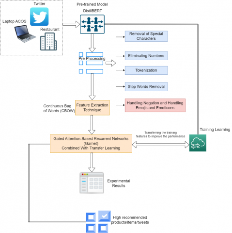
DistilBERT extends the well-known BERT (Bidirectional Encoder Representations from Transformers) model. The transmission-based model captures a massive corpus of text data to understand word context and meaning.  DistilBERT is a smaller, faster version of BERT better suited for real-world applications with limited computational resources. CNNs, on the other hand, are DL models that have been widely applied to image processing tasks. However, their use in NLP, particularly for text classification tasks such as sentiment analysis, has yielded promising results. CNNs are particularly good at extracting local patterns and features from input data, which helps identify critical sentiment-bearing words and phrases in a given text. The proposed model's overall architecture is depicted in Figure 1.

Combining DistilBERT with CNN and leveraging transfer learning has proven to be an effective method for improving sentiment analysis performance. Transfer learning entails using pre-trained models, such as DistilBERT, and fine-tuning them for a specific task, such as sentiment analysis. It enables the model to benefit from pre-trained knowledge of language representations before focusing on learning sentiment-specific features from the target dataset. In this paper, a combined approach shows the strengths of DistilBERT and CNN and transfer learning. By combining DistilBERT's context-aware language understanding with CNNs' local feature extraction capabilities, our model can effectively capture the nuances and intricacies of sentiment expression in textual data. Transfer learning also allows us to save time and resources while training models, making it a practical and efficient solution for SA on large-scale datasets.

The following steps show the training on sentiment datasets.

Step 1: Preprocess the text data

Tokenize the input text into word pieces.

Add special tokens like [CLS] (start token) and [SEP] (end token) to mark the beginning and end of the text. Pad or truncate the sequences to ensure a fixed length.

Step 2: DistilBERT Embeddings

Pass the preprocessed tokens through the DistilBERT model to obtain word embeddings.

Step 3: Combine CNN with DistilBERT embeddings

For each layer of DistilBERT, extract the corresponding word embeddings.

Apply 1D convolutions with multiple filters (kernels) to the embeddings.

Apply ReLU to the convolution outputs.

Perform max-pooling over the temporal dimension (sequence length) to obtain a fixed-size representation.

The equations for the CNN layer can be described as follows:

Let E be the word embeddings obtained from the DistilBERT model for a single layer, where $\mathrm{E}=\left[\mathrm{e} \_1, \mathrm{e} \_2, \ldots, \text{e_n}\right]$, n being the sequence length (number of tokens).

Let K be the number of filters (kernels) used in the CNN layer, and f be the filter size (width of the filter). Typically, f is smaller than the sequence length.

The convolution operation for each filter k is defined as:

$\operatorname{conv}_{\mathrm{k}}=$ Conv1D(filter_size $=\mathrm{f}$, activation $=$ 'relu')(E)

The output of the convolution operation will have a shape of (n - f + 1, K).

Next, we apply max-pooling over the temporal dimension to get a fixed-size representation:

pooled $\mathrm{k}=$ MaxPooling1D(pool_size $=\mathrm{n}-\mathrm{f}+1)$ (conv_k)

This will result in pooled $_{\mathrm{k}}$ having a shape of (1, K).

Step 4: Sentiment Classification

Concatenate or average the $_{\mathrm{k}}$ representations from all the layers.

Feed the combined representation through a FCL.

The final layer's output will be passed through a softmax activation to obtain probabilities for different sentiment classes (e.g., positive, negative, neutral).

1.png

Figure 1. Overall architecture of ERS

3.2 Experimental evaluation based on training and testing accuracy with loss

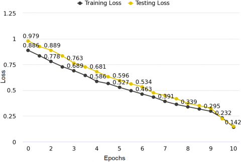
In this section, three datasets such as Laptop-ACOS, Restaurant and Twitter were used to evaluate the training and testing loss with accuracy. The proposed pre-trained model design for training the sentiment analysis data; the training loss is typically lower than the testing loss. However, both metrics must monitor during model development to ensure that the model does not over fit the training data and performs well on unseen data. Over fitting may indicate a large gap between training and testing loss, which can be addressed using techniques such as regularization or adjusting the complexity of the model.

2.png

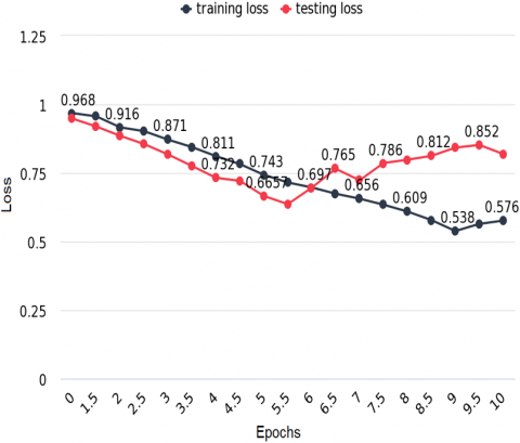
Figure 2. Training loss and testing loss for Laptop-ACOS

Figure 2 depicts the training and testing losses over ten epochs. The training and testing losses are the same at 0.968. The training loss is low when DistilBERT is used as the training model. The Laptop-ACOS dataset has a low testing loss. Low training loss indicates that the proposed approach honourably predicts the training data. An intense training loss suggests that DistilBERT captured the patterns and connections in the training dataset and can generalize well to the data seen during training.

3.png

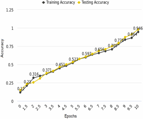
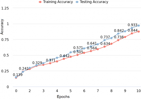
Figure 3. Training accuracy and testing accuracy Laptop-ACOS

Figure 3 initializes the training and testing accuracy for the Laptop-ACOS dataset. The training accuracy is 0.864 and the testing accuracy is 0.946. The high training accuracy indicates that the model learned and remembered the patterns in the training data. It can accurately classify the sentiment of the examples on which it was trained. However, high training accuracy does not always imply that the model will perform well on unlabeled data.

4.png

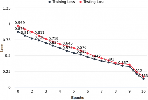
Figure 4. The loss values for the training and testing phases were computed for the Restaurant dataset

5.png

Figure 5. The accuracy scores were measured for both the training and testing sets of the Restaurant dataset

6.png

Figure 6. Training and testing loss for twitter dataset

7.png

Figure 7. Training and testing accuracy for twitter dataset

A high training loss suggests that the model struggles to effectively learn from the training data. This could indicate that the model requires assistance in discerning the underlying patterns within the data or that it may be overfitting to the training set. Overfitting arises when a model becomes excessively focused on capturing noise or specific examples within the training data, leading to diminished performance when applied to unseen data.

Figure 4 illustrates the training and testing loss for the Restaurant dataset, both of which are remarkably low and Figure 5 shows the high training and testing accuracy which represents the model fit for learning more significant factors from the dataset.   

Figure 6 indicates the low training loss which is 0.142 and the testing loss is 0.142 for the Twitter dataset. These values represent the low training and testing loss. Figure 7 represents the high training and testing accuracy which indicates the better performance of the model.

3.3 Pre-processing technique

For sentiment analysis, effective pre-processing of the dataset is crucial to ensure accurate and meaningful results. Here are some advanced pre-processing techniques that can help improve the performance of SA models:

The following functions used to remove the punctuation marks, symbols, emojis, and any other non-alphanumeric characters.

def remove_special_characters(text):

    # Define the pattern for identifying special characters and symbols

    # The regular expression [^\w\s] matches any non-alphanumeric character (excluding whitespace)

    pattern = r'[^\w\s]'

    # Use the re.sub() function to replace all occurrences of the pattern with an empty string

    clean_text = re.sub(pattern, '', text)

      return clean_text

# Example usage:

222.png

cleaned_text = remove_special_characters(text_with_special_characters)

print(cleaned_text)

Output: Hello this is a sample text with special characters

In the preceding code, we use Python's re.sub() function to replace all occurrences of memorable characters and symbols in the input text with an empty string, effectively removing them. Remember that eliminating special characters may change the meaning of the text, mainly when dealing with emoticons, acronyms, or text-based communication such as social media posts. As a result, it's critical to think about the context and requirements of your specific sentiment analysis task. To further preprocess the data before performing sentiment analysis, you can convert all text to lowercase and remove extra whitespaces.

Eliminating numbers: In many cases, numbers do not contribute to sentiment analysis, so removing them can simplify the data.

def remove_numbers_from_text(text):

    # Use regex to replace any sequence of digits with an empty string

    result = re.sub(r'\d+', '', text)

    return result

# Example usage:

text_data = "This is an example text with 123 numbers 4567 scattered 89 throughout."

cleaned_text = remove_numbers_from_text(text_data)

print(cleaned_text)

This is an example text with numbers  scattered  throughout.

In this example, the function remove_numbers_from_text takes a text as input and uses the re.sub method from the re module to replace any sequence of digits (\d+) with an empty string. This effectively removes all numbers from the input text.

Tokenization:

Word Tokenization: The data split into words or tokens. It is mainly used to develop the word vocabulary for the model.

Sentence Tokenization: Divide the text into sentences, especially in cases where the sentiment analysis is at the sentence level.

Stopword Removal:

Remove common stopwords (e.g., "and," "the," "is") as they appear frequently in text but usually don't carry significant sentiment information.

Handling Negation:

Identify negation words like "not," "no," "never," etc., and modify the following words to represent negated sentiment properly (e.g., "good" becomes "not_good").

Handling Emojis and Emoticons:

Convert emojis and emoticons to textual representations to preserve their sentiment meaning.

N-grams and Feature Engineering:

The contextual data is created by n-grams which improve the performance in terms of text understanding. 

Word2Vec is a word embedding method representing dense vectors in continuous vector space. This method introduces two types of techniques: Continuous Bag of Words (CBOW) and Skip-gram.

3.4 Feature extraction

3.4.1 Continuous Bag of Words (CBOW):

From the associated words the CBOW predicts the target word. The formula for CBOW can be explained as follows:

Let:

Vocab_size: Total number of unique words in the vocabulary

Word vector size: The dimensionality of the word embeddings (e.g., 100, 300)

Context window size: The number of words on both sides of the target word considered as context (e.g., 2, 5)

For each target word w(t) in the context window, the CBOW objective is to maximize the average log probability of predicting w(t) given its context words

$\mathrm{w}(\mathrm{t}-$ context_window $), \ldots, \mathrm{w}(\mathrm{t}-1), \mathrm{w}(\mathrm{t}+$ 1), $\ldots, w(t+$ context_window $)$ :

CBOW formula:

$\begin{aligned} & maximize \Sigma(\log \mathrm{P}(\mathrm{w}(\mathrm{t}) \mid \mathrm{w}(\mathrm{t}-\text { context_window }), \ldots, \mathrm{w}(\mathrm{t}-1), \mathrm{w}(\mathrm{t}+1), \ldots, \mathrm{w}(\mathrm{t}+ \text { context_window })))\end{aligned}$

Skip-gram:

In contrast, skip-gram attempts to predict context words given a target word. The formula for the Skip-gram is as follows:

For each target word w(t) in the context window, the Skip-gram objective is to maximize the average log probability of predicting the context words w(t-context_window), ..., w(t-1), w(t+1), ..., w(t+context_window) given the target word w(t):

Skip-gram formula:

$\operatorname{maximize} \Sigma(\log \mathrm{P}(\mathrm{w}(\mathrm{t}-$ context_window $), \ldots, \mathrm{w}(\mathrm{t}-$ 1), $\mathrm{w}(\mathrm{t}+1), \ldots, \mathrm{w}(\mathrm{t}+$ context_window $) \mid \mathrm{w}(\mathrm{t})))$

Word2Vec achieves this goal by iterative training on a large corpus of text data with neural networks, typically a shallow neural network with one hidden layer. The word vectors that result capture semantic relationships between terms, allowing for a variety of NLP tasks.

Figure 8 showcases how CBOW and Skip-gram methods are represented for feature extraction.

8.png

Figure 8. Architectures CBOW and Skip-gram

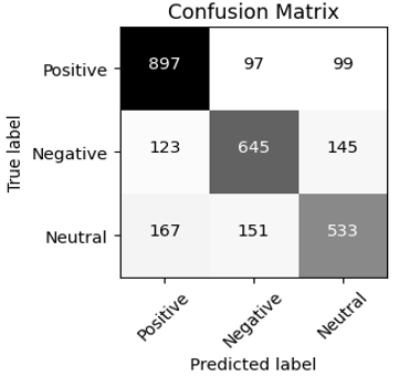
This section outperforms individual classifiers and traditional single-model approaches for sentiment analysis. We ran a series of experiments on a diverse and representative dataset that shows the performance of ERS for sentiment analysis. The three datasets comprise user-generated content from social media, product reviews, and online forums, and the sentiments are labeled as positives, negatives, and neutrals.

Table 3. Confusion matrix for Laptop-ACOS dataset

Table 4. Assessing the performance disparity between established and proposed algorithms on the Laptop-ACOS dataset

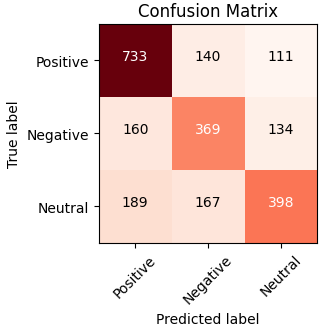
Table 5. Confusion matrix for Restaurant dataset

10.png

Figure 10. Count values for the Laptop-ACOS dataset

11.png

Figure 11. Comparative evaluation of various DL models alongside the proposed model on the Laptop-ACOS dataset

12.png

Figure 12. Confusion matrix count values for Restaurant dataset

13.png

Figure 13. Performances of the Restaurant dataset in terms of metrics

Table 6. Performance of models based on the count values

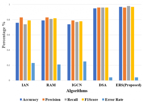
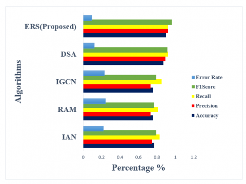
Table 3 shows the count values obtained from the confusion matrix that shows the comparison between list of DL algorithms. Compared with all the algorithms, the TP values are 1115, which is high for ERS, and the other values are TN obtained at 901, FP received at 40, and FN received at 19. IAN got a low performance in terms of count values. Figure 10 shows the performance using the visualization of count values - all these values obtained for the Laptop-ACOS dataset. The performance analysis from these count values with the parameters is shown in Table 4. Among all the algorithms, the version of the ERS shows high accuracy with 0.9716. The ERS offers a low error rate compared with the IAN model. High accuracy is obtained based on the overall positives by calculating actual and predicted values that are the same. High accuracy represents the strength of the proposed model, and low accuracy represents the drawback of the model. Figure 11 shows the comparative performances obtained from Table 4.

Table 5 shows the count values of the Restaurant dataset based on the confusion matrix. Figure 12, comparative count values among the list of DL algorithms. Table 6 and Figure 13 indicate the comparison between the list of models based on obtained results from the confusion matrix. ERS shows high for the Restaurant dataset with the accuracy of 0.9033 which is high among all the other models, and a low error rate of 0.0967.

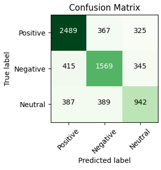
Table 7 and Figure 14 show the count values of overall performances that are obtained from confusion matrix. Table 8 and Figure 15 represent the performances of list of algorithms based on parameters given in Table 8. Among all the results the proposed approach obtained the high results compare with the existing models. The accuracy is 0.911 which is high compare with existing algorithms.

Table 7. Count values obtained from the twitter dataset for list of algorithms

Table 8. Performances of algorithms based on the given parameters for Twitter dataset

Table 9. Overall performances of sentiment analysis for list of algorithms in terms of positive, negative and neutral for Laptop-ACOS

14.png

Figure 14. Confusion matrix for Twitter dataset

15.jpg

Figure 15. Performance in terms of parameters

16.png

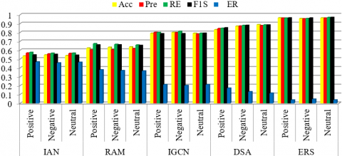
Figure 16. Comparative assessment of the overall performance of DL models on the Laptop-ACOS

17.png

Figure 17. Overall comparative performances of DL Algorithms for Restaurant dataset

18.png

Figure 18. Overall comparative performances of DL algorithms for the twitter dataset

Table 9 shows the overall performances of the list of algorithms by showing the sentiments like positive, negative and neutral. Among all these algorithms the high sentiments are obtained by the proposed ERS algorithm. Figure 16 shows the comparative performances in terms of sentiments with performance metrics. All these are applied to the Laptop-ACOS dataset.

Table 10 and Figure 17 show the performances in terms of positive, negative and neutral values obtained from the proposed approach.

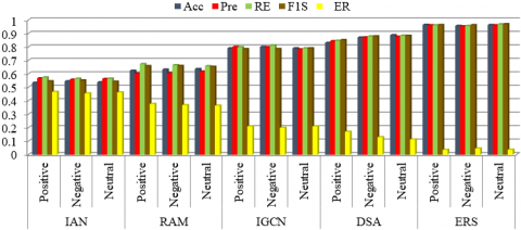
Table 11 and Figure 18 show the overall performances of the sentiments based on the obtained results. The sentiments are obtained based on the  positive, negative and neutral values measured by using the count values.

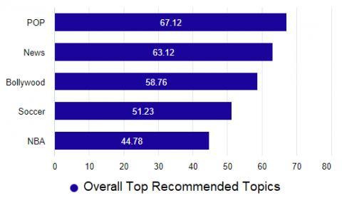
Figures 19-21 show the top recommended laptops, Restaurant-ACOS and Twitter data analysis is given in this section.

Table 10. Overall performances of list of algorithms in terms of positive, negative and neutral for Restaurant dataset

Table 11. Overall performances of list of algorithms in terms of positive, negative and neutral sentiments for Twitter

19.png

Figure 19. Overall percentage of Top-5 laptops based on SA

20.png

Figure 20. Overall percentage of Top-5 Restaurants based on SA

21.png

Figure 21. Overall percentage of top recommended topics in twitter data