Predicting Transport Mode in the Rabat Region: A Machine Learning Approach

The large population agglomeration that comprises a region of Rabat presents excellent challenges related to the development of an infrastructure capable of accommodating the traffic within this agglomeration and thus achieving flexibility and ease of movement, which requires appropriate planning to accomplish this challenge. The Rabat area is an essential urban pole with more than four million residents and needs, primarily, the coordination of efforts for a shared vision that contributes to the strengthening of infrastructure in the topic of urban transport and the development of forms of mobility, thus achieving a more flexible flow and more significant result. In addition, the center of Rabat remains the destination of most of the trips made in the aggregation. This means that thought must be given to ensure the fluidity of trips and target densely populated urban areas. In the context of daily mobility, which entails researching how people and goods move around a city daily. This includes the movement of vehicles, bicycles, and pedestrians and the infrastructure and systems that support these movements. One approach to studying and improving daily mobility is multi-agent systems (MAS). MAS are a type of system in which multiple agents interacted with each other to reach same goal. In addition, in the context of everyday mobility, MAS agents could represent individual vehicles, traffic lights and pedestrians. These agents would communicate and make decisions to avoid crashes, improve traffic flow, and lessen congestion. The effectiveness and safety of transportation in a city may be increased by employing MASs for daily movement. In this topic, we present a model to support urban decisions in the region of Rabat based on a machine learning algorithm and multi-agent system model. Decentralized control, hybrid control, game-theoretic approach, machine learning-based approach, and formal approaches are a few of the ways that may be used to achieve it. Machine learning has altered our perspective on daily mobility. Many aspects of our everyday mobility have been improved thanks to machine learning algorithms and technological improvements. Machine intelligence has emerged as a crucial tool for enhancing our everyday journey, from streamlining traffic to anticipating travel patterns. Additionally, the development of intelligent transportation systems has benefited from machine learning. By learning from user behavior, these systems can provide personalized recommendations for modes of transportation, such as suggesting the most efficient combination of public transit and ride-sharing services. Machine learning algorithms can also analyze data to create models supporting public transport exploitation, ensuring better service and minimizing delays. Traffic management is one of the critical ways that machine learning is used in daily mobility. Machine learning algorithms can accurately predict traffic congestion and suggest alternative routes in real time by analyzing vast amounts of data from traffic sensors, GPS systems, and historical patterns. This saves commuters valuable time, reduces fuel consumption, and lowers carbon emissions, contributing to a more sustainable transportation system. Decentralized control distributes decision-making power among the agents; centralized control relies on a central system or controller; hybrid management combines elements of both; the game-theoretic approach models agents as players in a game; a machine learning-based approach uses algorithms to learn and make predictions, and formal methods use mathematical techniques to verify system properties. The system's unique requirements and other factors like technological capability and moral ramifications determine the approach to use. In this study, we crafted a model within his research using four machine-learning algorithms to forecast individuals' transportation modes from the survey data supplied by HCP [1]. The results produced by the model can provide valuable insights to both the general public and decision-makers, aiding in formulating response strategies and resilience plans aimed at mitigating the effects of challenges on daily mobility. The primary contributions of this article are organized as follows: Section 2 introduces related work on solving Daily Mobility problems with multi-agent systems and machine learning models. Section 3 describes our proposed four algorithms that have been implemented (KNN, SVM, net-RBF, and BNN) in which we have used labeled data to implement the model developed and to be able to predict mode transport. Section 4 showcases the results achieved; comparing them with those obtained using the traditional multinomial logit model. The conclusion is then reached, followed by exploration of potential future extensions.

3.1 Dataset and attributes: Daily mobility in Rabat region and mode choices for displacement

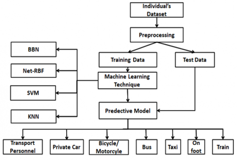
In this research, we employed individual-level data obtained from the HCP (High Commission for Planning). This census, initiated in 2014, offers a representative sample of the Rabat region's population, covering various demographic and socioeconomic attributes including 'Level of study, Age, the aggregate level of study, large group profession, professional status, activity sector, workplace, and mode of transport'. The dataset comprises 100,000 instances specific to the Rabat region. Table 1 outlines the individual dataset, consisting of 8 attributes grouped into 7 class features representing distinct modes of transportation: Transport Personnel, Private Car, Bicycle/Motorcycle, Bus, Taxi, on foot, and Train. The second phase involves data preprocessing, a critical step aimed at preparing and changing data to format identical to train a machine learning model. Given the diverse sources of training and testing datasets and the presence of missing values, this step includes the application of normalization and standardization techniques to ensure that numerical data is consistently and comparably scaled. The third stage involves identifying the nature of the target variable. In our research, the target variable is categorical, specifically used for classifying the transport mode. The fourth phase entails to divide the dataset to train and test sets. This division is performed to ensure that both training and testing datasets contain properly regulated analysis values, mitigating the risk of overfitting or under fitting. The final stage involves utilizing the training subset of the dataset to train machine learning models. This process enables the model to learn and generalize from the provided data. The parameters generated during this phase are subsequently employed in the final machine learning model, which is fine-tuned by optimizing the settings of each method to achieve the highest accuracy when making predictions during testing. The complete process is shown in the following Figure 1.

Table 1. Rabat region individual's dataset attributes

11.png

Figure 1. Proposed process of model mode travel predicted

3.2 Machine learning algorithm

Below is an explanation of this comparative research's various machine-learning methods.

3.2.1 k-nearest neighbors: KNN

The KNN or k-NN, it is a straightforward, nonparametric, supervised learning classifier, it is used to address classification and regression problems. One of the most straightforward and intuitive algorithms in machine learning is considered.. It is a good yet inefficient algorithm that waits until it receives the training sets before starting to train as stated by Zhang et al. [16].

The fundamental concept of K-Nearest Neighbors (KNN) is to identify the K closest data points in the training set to a specified test data point. In succession, either the majority class or the average of the labels from these K nearest neighbors is used to classify or predict the target to the test data.

Here are the steps for the KNN algorithm:

• Choose the value of k: k is the number of nearest neighbors that will be used to classify or predict the target value of a given test data point.
• Calculate the distance: It is between the test data point and all data points in the training set. While the Euclidean distance is the most frequently employed metric, various other distance metrics can also be considered. With X and Y be the respective coordinate points ((X₁,......, X_n), (Y₁,......., Y_n)) in a relevant space:

$D(x, y)=\sum_{i=1}^n\left(x_i-y_i\right)^2$                 (1)

• Find the k nearest neighbors: Choose K data points from the train dataset that exhibit the minimal distances on the test dataset, as determined by the selected distance metric.
• Classify or predict the target value: if the task is classification, assign the majority class label among the k nearest neighbors to the test data point. If the task involves regression, which calculates the average of the estimated values of the nearest neighbor K-factor values.
• Returns the predicted values: return the predicted target value for the test data point.

3.2.2 Support vector machine: SVM

It is an algorithm, widely utilized in tasks such as: a classification, regression and outlier detection. It is a supervised learning algorithm, aiming to determine the optimal hyper plane that maximizes the margin between the two classes within the data set, as outlined by Abdar and Makarenkov [17]. By positioning this hyperplane effectively in an n-dimensional space, SVM seeks to achieve optimal generalization capabilities, as highlighted by Osman [18].

As a result, the equation below serves as the definition of the ideal choice function:

$y=\operatorname{sign}(f(x))=\operatorname{sing}\left(\sum_{i=1}^n w_i \cdot x_i+b\right)$           (2)

With: $\left(x_1, y_1\right) \ldots \ldots \ldots\left(x_n, y_n\right) \in I R$. 

Here are the steps for the SVM algorithm:

• Data preparation: convert the data into a feature matrix X and target vector y, where X contains the features of each data point, and y contains the class labels
• Select the kernel: It determines the shape of the decision boundaries and the model's capacity to capture intricate patterns within the data.The choice of kernel depends on the nature of the data and the problem and hand.
• Training the SVM: it involves the process of teaching the algorithm to obtain the optimal hyper plane that best divides data samples belonging to different classes.
• Testing SVM: Once SVM has been trained, it can estimate the class labels of fresh data points. This is done on applying the trained SVM model to the feature matrix X of the new data points.
• Evaluation: Cross-validation or a validation set should be used to assess the SVM's performance. Accuracy, precision, recall, and F1 score are typical classification problem assessment criteria.

3.2.3 Artificial neural network multilayer perceptron: net-RBF

As elucidated by Broomhead and Lowe [19], an artificial neural network (ANN) with a radial basis function (RBF) employs radial basis functions as activation functions within its hidden layer. This ANN-RBF model operates under the assumption that the output for input patterns resembling a given input x will likely correspond closely to the expected value for x. Primarily utilized for pattern recognition and function approximation tasks, his architecture consists of three layers: an input layer, a hidden layer featuring radial basis functions, and an output layer. It uses its hidden layer to transform input data into a higher-dimensional space. It is connected to each neuron in the hidden layer, typically a Gaussian function mathematical centered at a specific point in the input space. In the Figure 2, we present RBF Neural Network architecture.

2.png

Figure 2. Multilayer perceptron architecture in artificial neural networks

The value of the output is determined based on the input using the following equation:

$y=\sum_{i=1}^h w_i . \emptyset(\|\mathrm{x}-\mathrm{ci}\|)$        (3)

With $h$ is the number of hidden neurons, $w_i$ and $c_i$ the weight associated and the center of the $i$-th RBF. Furthermore, $\varnothing$ is a radial basis function (RBF). During the training process, the objective is to optimize the two sets of values, namely $w$ and $c$.

3.2.4 Bayesian belief network: BBN

It is a collection of random variables with their probabilistic interconnections. It is typically represented as a tuple (G, P), additionally G denotes a directed acyclic graph (DAG) accompanied by a node corresponding to each variable in the model, as described by Broomhead and Lowe [19]. Meanwhile, P represents a multivariate probability distribution defined for each variable. In a Bayesian Belief Network, a set of nodes, each corresponding to variables within the system under investigation, embodies the key factors influencing the phenomenon being studied. Each node encompasses a set of mutually exclusive states. The network comprises directed links that encode conditional dependencies among these nodes, delineating the relationships between variables. Additionally, each node incorporates a set of probabilities that specify the likelihood of it being in a particular state based on the states of its parent nodes. To illustrate, consider a scenario with three nodes. Can be representing the relationship among these variables by this following expression mathematic:

$\mathrm{P}(\mathrm{B} / \mathrm{A})=\frac{\mathrm{P}(\mathrm{B}, \mathrm{A})}{P(A)}$              (4)

In the equation provided, P represents a multivariate probability distribution.

It is a powerful tool for modeling complex systems, such as those involving human behavior, because it allows for efficient reasoning and inference. In studying individual behavior, a Bayesian belief network can represent the various factors that influence a person's actions. For example, a network could include variables such as a person's mood, the time of day, the location they are in, and any external stimuli they are exposed to. The network would also include the probabilistic relationships between these variables, such as the likelihood that a person will be in a good mood if they have had enough sleep the previous night. It is possible to make predictions about a person's behavior based on the values of these variables by this model. For example, if a person is in a crowded public place and is exposed to loud noises, the network could predict that they will likely become agitated. This prediction could be used to inform decisions about how to manage the situation best, such as by providing a quieter area for the person to retreat to. In addition to making predictions, a Bayesian belief network can identify the most important factors influencing a person's behavior. Analyzing the network makes it possible to determine which variables have the strongest effects on the outcome of interest. This information can benefit the creation of interventions that target the most influential factors to achieve the desired behavior change. Overall, a Bayesian belief network helps study individual behavior because it allows for modeling complex, probabilistic relationships between multiple variables. It can be used to predict behavior and identify the key factors that influence it, which can inform the development of effective interventions.

In machine learning and artificial intelligence, Bayesian Belief Networks (BBNs) are frequently employed to model uncertain and intricate domains. This approach has demonstrated success in various domains, including medical diagnostics, decision support systems, semantic search, and bioinformatics, as evidenced by studies conducted by Andersen et al. [20-22].

In the realm of machine learning, BBNs find utility in diverse tasks such as classification, anomaly detection, missing data imputation, and feature selection, as highlighted in the research conducted by Chen et al. [23]. These networks can be trained from data by amalgamating expert knowledge with data-driven learning techniques.

In this section, we present our experimental findings. Employing the renowned Weka tool, we conducted supervised learning utilizing four distinct machine learning algorithms: KNN, BBN, SVM, and net-RBF. These algorithms were implemented using the popular Scikit-learn Python library. To evaluate the performance of the machine learning model, we utilized both Train/Test split and Cross-validation techniques. This approach aids in gauging the model's effectiveness on unseen data and mitigating overfitting, wherein the model merely memorizes the training data instead of identifying underlying patterns.

The dataset was split randomly, with 80% of the individuals' dataset destined to train the model, while the remaining 20% to test. The training set utilized for model training, the validation set for tuning hyper parameters and model selection, and the test set for final evaluation. The initial results obtained from the Train/Test Split are presented in Table 3.

As a secondary outcome, as depicted in Table 4, we employed 10-fold cross-validation, allocating 80% to train and 20% to test.

Table 3. Assessing metrics utilizing a partition of train/test data

Table 4. Performances algorithms comparison

3.png

Figure 3. Comparative diagram of algorithms proposed concerning evaluation criteria: Accuracy, Precision, Recall, F1- score

4.png

Figure 4. The net-RBF model's architecture was applied to predicting employers' transport modes in the Rabat region

5.png

Figure 5. The ROC curve net-RBF mode

In Figure 3, we will show the comparative performance of these algorithms.

To better understand the model's efficiency, Figure 4 illustrates the architecture of the net-RBF, delineating its input, hidden, and output layers. Meanwhile, Figure 5 showcases the ROC curve for our classifiers, specifically highlighting the precision of each classifier when employing the net-RBF algorithm. By presenting the ROC curve, we offer a visual depiction that elucidates the performance disparities among different classifiers, aiding in a comprehensive understanding of their efficacy.