Chaerur Rozikin*![]() | Agus Buono
| Agus Buono![]() | Sri Wahjuni
| Sri Wahjuni![]() | Chusnul Arif
| Chusnul Arif![]() | Widodo
| Widodo![]()
© 2023 IIETA. This article is published by IIETA and is licensed under the CC BY 4.0 license (http://creativecommons.org/licenses/by/4.0/).
OPEN ACCESS
Diseases of melon plants can cause losses to farmers, such as reduced productivity or even death of melon plants. Downy mildew (DM) is a well-known fast-spreading disease affecting the leaves of melon plants. It is important to determine the level of severity of DM leaf disease so that farmers can take preventive measures according to the severity of DM disease that infects the leaves. Determining the severity of DM disease can be done with experts, but experts have limitations, namely, the availability of experts, and not all areas have leaf disease experts. The stages of this research were data acquisition, preprocessing, feature extraction, feature selection, and classification. Data were taken directly from farmers' gardens and then pre-processed. Color, texture, edge, and entropy features were extracted to obtain the combined feature values. Combined features are prone to redundant and irrelevant features; therefore, feature selection must be performed to obtain the best features. This research proposes an integration concept between the analysis of variance (ANOVA) and artificial bee colony (ABC) optimization, which is named AVABC, and is used as a feature selection algorithm. The test results for the search process time for the eight best features using the AVABC algorithm took 05 minutes 23 s, whereas the test results for the search process time for eight features using ABC with the accuracy model fitness function took 20 h 08 min 55 s. The AVABC feature selection algorithm has the advantage of faster search time for the eight best features.
analysis of variance (ANOVA), artificial bee colony (ABC), ANOVA-ABC (AVABC) algorithm, downy mildew classification, feature selection, melon leaf disease, precision agriculture optimization
Agricultural productivity is highly dependent on the quality and quantity of agricultural products, particularly melon crops [1]. Melons are fruit commodities with a high selling price, so many farmers choose to cultivate melon plants. However, cultivating melons is difficult because many diseases can attack melon plants. Diseases of melon plants can occur in fruits, leaves, stems, and roots [2]. Several types of diseases that commonly occur in melon plants include bacterial fruit blotch, Anthracnose, Powdery mildew, Fusarium wilt, root-knot nematodes, downy mildew, melon fruit flies, and melon-cotton aphids [3]. The most well-known and fast-spreading disease in melon plants is downy mildew [4]. Diseases of melon plants can cause losses to farmers, such as reduced productivity or even plant death [5]. Diseases of melon plants, especially on infected plant leaves, can be recognized by changes in the color, shape, edges, and surface texture of the leaves. Melon leaves experience changes according to the level of disease development that attacks the leaves of the melon plant. Therefore, it is important to determine the severity of downy mildew disease on the leaves so that farmers can take preventive measures according to the severity of the disease affecting the leaves of melon plants.
One of the computer technologies currently being developed to determine the severity of disease in melon leaves is image processing (IP) and machine learning (ML). Image processing technology is used to recognize objects in the form of images of leaves, whereas machine learning is used to classify the severity of disease on melon leaves. The use of IP and ML allows the determination of the severity of the disease on melon plant leaves to be carried out quickly and accurately so that it can assist farmers in taking preventive measures appropriate to the severity of the disease. In general, the stages of classifying the severity of leaf disease using IP and ML include data acquisition, pre-processing, feature extraction, feature selection, and classification [6].
The VGG16 deep learning method was used to classify the severity of blight on tea leaves into two levels: mildly affected leaves and severely affected leaves. The model was tested and achieved an average accuracy of 84.5% [7]. The use of deep learning with the resnet architecture has enabled the classification of the severity of leaf disease on tomato plants into healthy leaves, leaves affected by mild disease, and leaves affected by severe disease, with an average accuracy of 88.2% in the model testing results [8]. The BLSNet model was utilized to categorize the intensity of bacterial leaf streak disease in rice plants into five stages: stage 0, with no signs of disease; stage 1, with less than 10% affected areas; stage 2, with 11-25% affected areas; stage 3, with 26-45% affected areas; stage 4, with 46-65% affected areas; and stage 5, with more than 65% affected areas. The model accomplished an overall accuracy of 98.2% [9].
To classify the severity of disease in melon plant leaves, four categories of melon leaf image data are required: healthy leaves, leaves affected by mild downy mildew disease, medium grade downy mildew disease, and severe grade downy mildew disease. Image data of melon leaves photographed using a smartphone in a farmer's garden under natural conditions [10]. Next, the leaf image data will go through a pre-processing stage, where the images are cropped and resized to make them uniform, and the color conversion will be carried out from RGB to Grayscale [11]. The next stage is feature extraction, where features such as color, texture, Shannon entropy, and edge detection are extracted from the melon leaf image. The results of these feature extractions were then combined into combined features. Combined features are susceptible to noise, such as redundant and irrelevant features, which can affect classification performance [12].
Feature selection can overcome the problem of redundant and irrelevant features. There are two feature selection techniques: filter- and wrapper-based. Filter-based methods are used to find the optimal features from the original features based on ranking. The advantage of the filter-based technique is that it is simple and computationally efficient, but it is unable to exploit the relationship between features, thereby reducing the overall level of accuracy. Examples of filter-based techniques used for feature selection are grid-search [13], Recursive Feature Elimination (RFE) [14], and elastic net [12]. Wrapped-based methods utilize classifier knowledge to determine the optimal feature subset using an evolutionary algorithm to identify optimal solutions by analyzing the search area of a set of solutions (population) [15]. Examples of wrapped-based techniques used for feature selection include partial swarm optimization (PSO) [16], ant colony optimization (ACO) [17], artificial bee colony optimization (ABC) [18], and exponential spider monkey optimization (ESMO) [19]. There are two disadvantages to using the classifier accuracy as a fitness function criterion. First, the feature selection method depends on the classifier model, that is, a feature subset that is ideal for one classifier model may not be suitable for another classifier. Second, the classifier must be retrained using an appropriate subset of features to obtain the fitness values. This type of fitness assessment technique increases computing time during the search and selection of the best features [20].
The ABC algorithm was introduced by Karaboga in 2005 [21]. In 2009, a comparative study of the ABC algorithm was carried out using genetic algorithms, particle swarm optimization algorithms, differential evolution algorithms, and evolution strategies, and the results showed that ABC performance was better or similar to other population-based algorithms, with the advantage of using fewer control parameters [22]. Implementation of the ABC algorithm for classification [23], ABC for solving sales problems [24], and ABC for selecting the best features [25]. The stages of the artificial bee colony optimization algorithm [26] and the ABC algorithm used for feature selection with a fitness function using an accuracy model were performed on the grape leaf dataset [27]. The experimental results of this research feature selection using ABC with an accuracy model fitness function have a weakness, namely that the feature selection process takes a long time. This study aims to create a feature selection model using the AVABC algorithm to select combined features, and the results of feature selection are the best features. Then, a classification process was conducted to determine the severity of downy mildew disease in melon leaves. The AVABC algorithm is an artificial bee colony (ABC) optimization feature selection algorithm with fitness assessment criteria based on analysis of variance (ANOVA). This study proposes an integration concept between variant analysis and artificial bee colony (ABC) optimization, which is called AVABC, and is used as a feature selection algorithm. The first stage of the AVABC algorithm collects images of melon leaves by photographing the leaves in melon farmers' gardens; second, pre-processing is performed to cut and resize the melon leaf images so that the melon leaf image data are uniform; and third, the melon leaf image data is then carried out by extracting color, texture, edge, and feature features. entropy feature. The results of the feature extraction are combined features that are subjected to a feature selection process using the AVABC algorithm. In the fifth stage, a classification process was conducted to determine the severity of downy mildew disease in melon leaves. The feature selection stages using AVABC first generate combined features, then initialize the number of solutions and the number of features to be selected. Third, the fitness function for each solution is calculated. Fourth, we compare the probability of each fitness function and save the highest probability value. Fifth, one of the features from the old solution was replaced with new features obtained from the combined features. Then, the probability of the old solution is compared with that of the new solution, and a high probability value is saved. The results of the AVABC feature selection are the best feature dataset, and these features are used as inputs for the classification model.
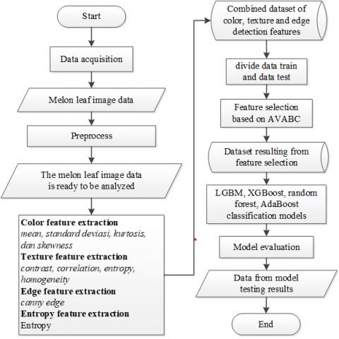
The methodology for classifying the severity of downy mildew disease on melon leaves, employing the AVABC feature selection, encompasses several stages as depicted in Figure 1.
2.1 Data acquisition
The acquisition of melon leaf data was conducted through a structured cultivation process. Melon plants were sown in a controlled manner from October 17, 2022, to December 20, 2022. The cultivation site was located in Sukatani village, within the Sukatani sub-district, Purwakarta district, West Java. Subsequently, the melon leaves were photographed using a smartphone camera directly in the farmer's garden. The technical specifications of the smartphone used for photography are detailed in Table 1.
A total of 1861 images of melon leaves were collected through this process. The grading of downy mildew disease on these leaves was performed with the collaboration of the plant protection laboratory. The specific criteria employed for the grading of downy mildew disease are outlined in Table 2.
The criteria for the grading of downy mildew disease were meticulously established, which guided the subsequent labeling of the collected melon leaf images. Detailed information regarding the labeling outcomes for each image is systematically presented in Table 3.
Figure 1. Research stages
Table 1. Smartphone specification
|
No. |
Name |
Specification |
|
1 |
Smartphone |
Infinix note 11 NFC |
|
2 |
Camera resolution |
triple camera 50 MP, f/1.6, (wide), PDAF, 2 MP, f/2.4, (depth) |
|
3 |
Operating sytem |
Android 11 |
Table 2. Criteria for the severity of downy mildew disease
|
No. |
Label of Grade Leaves Disease |
Criteria |
|
1 |
Healthy Leaves (HL) |
The surfaces of melon leaves did not show any symptoms of downy mildew disease. |
|
2 |
Downy Mildew Grade 1 (DMG1) |
The symptoms of downy mildew disease begin to appear on the surface of melon leaves until 20% of the melon leaf surface is infected. |
|
3 |
Downy Mildew Grade 2 (DMG2) |
The surface of the melon leaves is infected with downy mildew disease 20% until the surface of the melon leaves is infected with 40% of the surface of the melon leaves. |
|
4 |
Downy Mildew Grade 3 (DMG3) |
The surface of melon leaves is more than 40% infected with downy mildew. |
Table 3. Melon leaf image dataset
|
No. |
The Type of Disease |
Amount of Data |
|
1 |
Healthy Leaves (HL) |
665 Images |
|
2 |
Downy Mildew Grade 1 (DMG1) |
449 Images |
|
3 |
Downy Mildew Grade 2 (DMG2) |
253 Images |
|
4 |
Downy Mildew Grade 3 (DMG3) |
494 Images |
|
Total amount of data |
1861 Images |
|
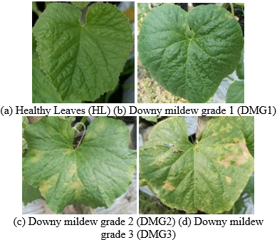
Labeling was meticulously conducted to categorize the melon leaves into four distinct groups: Healthy leaves, and leaves exhibiting signs of downy mildew at varying severity levels – grade 1, grade 2, and grade 3. Detailed visual representations of these categorizations are provided in Figure 2.
Figure 2. Examples of images of melon leaves affected by downy mildew disease
2.2 Preprocessing
In the preprocessing stage, the image data of melon leaves were subject to cropping and re-sizing. The original dimensions of the images, 2087 pixels × 2087 pixels, were altered to a standardized size of 128 pixels × 128 pixels post-cropping. This re-sizing was essential to remove extraneous objects and isolate the desired melon leaf image for analysis. Furthermore, a conversion of the image color from RGB to grayscale was performed to simplify the subsequent processing stages.
2.3 Feature extraction
Subsequent to preprocessing, feature extraction was undertaken to derive valuable information from the images. This study's feature extraction focused primarily on the aspects of color, texture, and shape. The methods employed in this phase included calculations for average color values, standard deviation, and skewness, as outlined in Eqs. (1-3) [27]:
Mean $=\frac{1}{M X N} \sum_{X=1}^M \sum_{y=1}^n M_{x y}$ (1)
Standart Deviation $=\sqrt{\frac{1}{M X N} \sum_{x=1}^M \sum_{y=1}^N\left(M_{x y}-m\right)^2}$ (2)
Skewness $=\frac{\sum_{x=1}^M \sum_{y=1}^N\left(M_{x y}-m\right)^3}{(M x N) \times S D^3}$ (3)
Color feature values extracted encompassed blue mean, green average, red average, blue standard deviation, green standard deviation, red standard deviation, blue kurtosis, green kurtosis, red kurtosis, blue skewness, green skewness, and red skewness. Histogram values were extracted using Eq. (4) [28], where represents the number of pixels at intensity levels:
$h\left(r_k\right)=n_k$ (4)
where, nk is the number of pixels with rk intensity levels.
Texture features aimed to ascertain distance and angle metrics through calculations of homogeneity, entropy, energy, contrast, and correlation (Eqs. 5-10) [29]:
Energy $=\sum_{i, j}(p(i, j))^2$ (5)
Correlation $=\frac{\sum_i \sum_j(i j) P(i, j)-\mu_x \mu_y}{\sigma_x \sigma_y}$ (6)
$\sum_{i, j} \frac{p(i, j)}{1+|i-j|}$ (7)
Contrast $=\sum_{n=0}^{N_g-1} N^2\left\{\sum_{i=1}^{N_g} \sum_{j=1}^{N_g} P(i, j)\right\},|i-j|=n$ (8)
Entropy $=-\sum_i \sum_j P(i, j) \log (P(i, j))$ (9)
Homogeneity $=\sum_{i, j} \frac{p(i, j)}{1+|i-j|}$ (10)
Texture features aimed to ascertain distance and angle metrics through calculations of homogeneity, entropy, energy, contrast, and correlation (Eqs. 5-10) [29]. GLCM feature values were extracted with variations in distance (1, 3, 5) and angles (0°, 45°, 90°, 135°).
Edge features were quantified using the Canny method, which entailed noise reduction via a Gaussian filter, as per Eq. (11) [30]:
$G(x \cdot y)=\frac{1}{2 \pi \sigma^2} \exp \left(-\frac{x^2+y^2}{2 \sigma^2}\right)$ (11)
The calculation of image gradient involved variables of distance (y and x) and the standard deviation of the Gaussian distribution (σ), with gradient magnitude (G) and orient angle (θ) computed using Eqs. (12) and (13):
$G=\sqrt{\left(G_x^2+G_y^2\right)}$ (12)
$\theta=\tan \left(\frac{G_y}{G_x}\right)$ (13)
where, Gx and Gy represent the horizontal and vertical gradients respectively.
Shannon posited that for quantifying the information content H(p) in a series of events p1, …, pn, three fundamental requirements must be met. Firstly, the H must exhibit continuity in the event series pi. Secondly, if all events pi possess equal probability, thus $p_i=\frac{1}{N}$, then H should be a monotonically increasing function of N, and H must exhibit additivity [31]. Adhering to these principles, Shannon entropy features in this study were extracted using Eq. (14):
$H(p)=-k \sum_{i=1}^N p_i \ln p_i$ (14)
The combined feature dataset, integrating color, texture, edge, and entropy features, was formulated using Eq. (15). This dataset incorporated color (DFColor), texture (DFTexture), edge (DFEdge), and entropy (DFEntropy) feature datasets:
DFCombined $=$ DFColor $\cup$ DFTexture $\cup$ DFEdge $\cup$ DFEntropy (15)
The study divided the combined feature dataset into training and test datasets, considering the impact of dataset distribution on model accuracy. Three scenarios were tested: 90% training and 10% test data (Scenario 1), 80% training and 20% test data (Scenario 2), and 70% training and 30% test data (Scenario 3) [32, 33]. Based on the findings, Scenario 3, with 70% training data and 30% test data, was selected for this research, as detailed in Table 4.
Table 4. Divided data train and test
|
No. |
Dataset |
Percentage |
Total Dataset |
|
1 |
A mount of dataset |
100% |
1861 images |
|
2 |
Train data |
70% |
1301 images |
|
3 |
Test data |
30% |
560 images |
2.4 Feature selection based on AVABC
The ABC algorithm, noted for its comparable or superior performance to other population-based algorithms while utilizing fewer control parameters, is adeptly suited for feature selection to isolate the most effective features. In this study, the ABC algorithm was adapted for combined feature selection, with a key modification in the fitness function utilizing ANOVA. ANOVA serves to analyze variances between features or to assess the extent of differences among them. Features exhibiting a high level of variance are deemed optimal. This research introduces a novel feature selection concept based on AVABC, which combines ANOVA and ABC optimization. The procedural steps of the AVABC algorithm are outlined in the following pseudocode.
|
Seleksi fitur menggunakan ABC dan fitness function ANOVA 1. Generate combined feature (CF). ###Employed Bee 2. Initialize the number of solutions (ST) and the number of features to be selected (SF) from the combined features (CF). 3. Initialize table T as many as i (i=1, 2, 3, …, ST), with feature f as many as j (j=1, 2, 3, …, SF) 4. Calculate the fitness function Fi for each table Ti using ANOVA 5. Save the Ti table with the best Fi ###Onlookers Bee 6. Find a new feature that can replace one of the fij of Ti which is taken from the combined feature vk (k=1,2, 3, …, CF) and is not yet in the Ti table using the formula $\mathrm{z}=\mathrm{x}+\phi(\mathrm{x}-\mathrm{y})$ where, x is the index number of fij, y is the index number of vk, ϕ is a random number, and z is the index of the new feature. 7. Calculate Fi from table Ti if feature fij is changed to vk[z] 8. If the Fi value from the table with feature vk[z] is better than the Fi value from the table with feature fij, replace fij with vk[z] 9. Repeat Steps 6 – 8 for the entire T table, with initial value i=0 10. Calculate the probability for table $T_i$ with the formula $p_i=\frac{F_i}{\sum_{n=1}^{S N} F_n}$ 11. Generate a random number r 12. If r is greater than pi, do Steps 6 – 8. If not, change the value of i to $i=(i+1) \% i$ then repeat Step 11 13. Do Steps 11 – 12 as many as ST, with initial value i=0 ###Scout Bee 14. Repeat Step 5 again to save the best table of exploration and exploitation results 15. If after several exploration and exploitation stages one of the Ti tables has not changed, do Steps 3 - 5 again. 16. Steps 6 – 15 are performed as many times as specified by the user |
2.5 Fitness function using ANOVA
The study categorizes the data into four classes: Healthy Leaf (HL), Downy Mildew Grade 1 (DMG1), Downy Mildew Grade 2 (DMG2), and Downy Mildew Grade 3 (DMG3). A score for each feature is calculated to determine its efficacy in differentiating these four classes. The numerator in this calculation is the distance between class distributions, computed using Eq. (16):
$\begin{aligned} & \text { Nominators }=H L\left(\bar{X}_{H L}-\bar{X}\right)^2+D M G 1\left(\bar{X}_{D M G 1}-\bar{X}\right)^2 \\ & +D M G 2\left(\bar{X}_{D M G 2}-\bar{X}\right)^2+D M G 3\left(\bar{X}_{D M G 3}-\bar{X}\right)^2\end{aligned}$ (16)
where, Class is the distance between class distributions, $H L$ is the healthy leaf class, $D M G 1$ is the $D M G 1$ class, $D M G 2$ is the $D M G 2$ class, $D M G 3$ is the $D M G 3$ class, $\bar{X}_{H L}$ is the $H L$ class average, $\bar{X}_{D M G 1}$ is the $D M G 1$ class average, $\bar{X}_{D M G 2}$ is the $D M G 2$ class average, $\bar{X}_{D M G 3}$ is the $D M G 3$ class average and $\bar{X}$ is the overall class average. The denominator is derived using a method akin to class-sample variance calculation. It involves dividing the sum of squares for each class by its population, followed by summing these values across all classes. The resultant aggregate is then divided by the total number of samples squared, as detailed in Eq. (17):
$S^2=\frac{\sum_{i=1}^n\left(x_i-\bar{x}\right)^2}{n-1}=\frac{1}{n-1} \sum_{i=1}^n\left(x_i-\bar{x}\right)^2$ (17)
where, $S^2$ is the sample class variance, $n$ is the amount of data, $x_i$ is the $i$ value of data, $\bar{x}$ is the average of the data. Employing the sample variance formula facilitates the derivation of Eq. (17), which is instrumental in calculating the denominator. This derivation leads to Eq. (18), outlining the steps for obtaining the denominator value:
$\begin{aligned} & S^2= \frac{1}{(D L-1)+(D M G 1-1)+(D M G 2-1)+(D M G 3-1)} \\ & \left(\sum_{i=1}^{H L}\left(H L_i-\bar{x}\right)^2+\sum_{j=1}^{D M G 1}\left(D M G 1_j-\bar{x}\right)^2+\right. \\ & \left.\sum_{k=1}^{D M G 2}\left(D M G 2_k-\bar{x}\right)^2+\sum_{l=1}^{D M G 3}\left(D M G 3_l-\bar{x}\right)^2\right)\end{aligned}$ (18)
Finally, the fitness function values for the classes are calculated using Eq. (19), which combines the numerator and denominator values:
fitness function $=\frac{\text { Nominator }}{\text { Dominator }}$ (19)
2.6 Evaluation model
The effectiveness of the feature selection process utilizing the AVABC algorithm was assessed by comparing its performance with that of traditional ABC and LGBM algorithms. Following the feature selection via AVABC, these optimal features were employed in the classification process using Random Forest, LGBM, and XGBoost algorithms. Key metrics such as running time, CPU usage, memory usage, and algorithm accuracy were evaluated. For accuracy measurement, a confusion matrix was utilized. This matrix is a tabular representation that categorizes the classification results into correct and incorrect predictions, thereby facilitating a comprehensive analysis of algorithm performance. The accuracy value was calculated based on the proportion of correctly predicted data, both positive and negative, in relation to the total dataset, as delineated in Eq. (20). This approach offers a quantifiable measure to compare the performance and efficiency of the selected algorithms:
Accuray $=\frac{T P+T N}{T P+F P+F N+T N}$ (20)
where, TP=True Positif, FP=False Negatif, TN=True Negatif, FN=False Negatif.
3.1 Collection and preprocessing of melon leaf image data
The collected melon leaf image dataset underwent initial preprocessing, which included cutting operations and resizing the images to a standard dimension of 128 × 128 pixels. This process was aimed at ensuring uniformity across the dataset. Subsequently, a color modification step was executed. The results of these preprocessing stages, demonstrating the transition from original images to cropped, resized, and color-altered forms, are illustrated in Figure 3.
Figure 3. Preprocessing results of the melon leaf image dataset
Table 5. Color feature extraction results
|
Leaf Sample |
meanR |
meanG |
meanB |
varR |
varG |
varB |
skewR |
skewG |
skewB |
|
HL |
131.217 |
131.427 |
131.225 |
3366.715 |
3493.703 |
3618.599 |
-0.0694 |
-0.0616 |
-0.0487 |
|
HL |
131.226 |
131.437 |
131.235 |
3366.722 |
3493.880 |
3618.663 |
-0.0695 |
-0.0618 |
-0.0489 |
|
HL |
131.241 |
131.449 |
131.240 |
3366.244 |
3493.523 |
3618.384 |
-0.0699 |
-0.0622 |
-0.0491 |
Table 6. Texture feature extraction results
|
Leaf Sample |
Energy_d1_00 |
Corr_d1_00 |
Diss_sim_d1_00 |
Homogen_d1_00 |
Contrast_d1_00 |
Entropy |
|
HL |
0.0130 |
0.8520 |
16.023 |
0.0840 |
555.354 |
7.386 |
|
HL |
0.0116 |
0.7800 |
22.277 |
0.0639 |
1034.979 |
7.524 |
|
HL |
0.0142 |
0.8580 |
14.946 |
0.0829 |
454.813 |
7.226 |
Table 7. Feature selection results based on AVABC
|
Index |
skewnessR |
skewnessB |
meanR |
meanG |
meanB |
varianceG |
skewnessG |
varianceR |
Class |
|
378 |
-0.0720 |
-0.0497 |
131.5638 |
131.8329 |
131.5877 |
3619.7397 |
-0.0652 |
3495.5400 |
DMG1 |
|
982 |
0.1085 |
0.1298 |
124.6073 |
125.2577 |
125.7566 |
3408.3501 |
0.1149 |
3302.8864 |
DMG3 |
|
943 |
0.1214 |
0.1395 |
124.4542 |
125.0188 |
125.5152 |
3406.2056 |
0.1269 |
3294.4720 |
HL |
|
1297 |
-0.4004 |
-0.2239 |
126.8684 |
123.9895 |
123.7734 |
2650.5545 |
-0.3064 |
2545.6441 |
DMG2 |
|
277 |
-0.0743 |
-0.0583 |
131.7243 |
132.0684 |
131.9097 |
3579.5105 |
-0.0704 |
3457.6593 |
DMG2 |
|
... |
... |
... |
... |
... |
... |
... |
... |
... |
... |
|
429 |
-0.0645 |
-0.0435 |
131.3671 |
131.6844 |
131.4623 |
3634.8864 |
-0.0583 |
3508.1477 |
DMG3 |
|
632 |
-0.0222 |
-0.0028 |
130.4342 |
130.8712 |
130.8638 |
3604.2445 |
-0.0168 |
3487.3431 |
HL |
|
94 |
-0.0671 |
-0.0485 |
131.2677 |
131.5152 |
131.3158 |
3508.7733 |
-0.0607 |
3382.0791 |
DMG2 |
|
1003 |
0.1031 |
0.1231 |
124.5322 |
125.1321 |
125.5820 |
3423.5103 |
0.1074 |
3318.2043 |
DMG1 |
|
695 |
0.0190 |
0.0386 |
128.7654 |
129.1889 |
129.2005 |
3572.5405 |
0.0230 |
3449.5549 |
HL |
3.2 Feature extraction
The color feature extraction from the melon leaf images led to the acquisition of various color feature values, including color distribution, texture, entropy, and edge features. Color features were calculated by averaging the values of red, green, and blue components. Additionally, color feature variants were extracted, resulting in skewness values for each color channel. In total, nine feature values were derived from the color feature extraction process. Table 5 presents three examples of melon leaf images used in this process.
Color distribution was analyzed using histograms, capturing the color distribution across each pixel and resulting in 512 color distribution features. Texture features were extracted using the Gray-Level Co-occurrence Matrix (GLCM), focusing on energy, correlation, dissimilarity, homogeneity, and contrast. These texture features were analyzed at various distances (1, 3, 5) and angles (0°, 45°, 90°, 135°), culminating in 60 texture features.
Entropy features, vital for managing uncertainty in disease classification into classes HL, DMG1, DMG2, and DMG3, were also extracted, enhancing the informational value between classes. Table 6 displays examples of melon leaf images from which texture and entropy features were extracted.
Edge features, identifying points of significant brightness changes, were extracted using the Canny edge detection method. The extraction yielded 256 distinct edge features.
3.3 Combined feature
The extraction of color, texture, entropy, and Canny edge features resulted in a comprehensive dataset comprising 521 color features, 60 texture features, 1 entropy feature, and 256 Canny edge features. These features were then amalgamated to form a combined feature dataset, totaling 838 features. This combined dataset is pivotal for the subsequent classification and analysis phases of the study.
3.4 Feature selection based on AVABC
The combined feature dataset was used to carry out a feature selection process based on AVABC (see Algorithm 1) to obtain a table with the eight best features. The first step is to prepare a combined feature dataset and then initialise a number of solutions and the number of features to be selected from the total number of combined features. First, the number of solutions and features is determined. In this study, the number of solutions was determined to be 10 solutions and 8 features. Next, the Employed Bee initialises 10 tables, with each table having eight features according to the number of solutions and features that have been determined. After obtaining 10 tables with eight features, the employed bee calculates the fitness value for each table using ANOVA, and the table with the highest fitness value is saved. Next, Onlooker Bee searches for new features in the combined features, which can replace one of the eight features in the 10 tables, and search for features that replace those not yet in the 10 tables using the equation $z=x+\phi(x-y)$ . Onlookers Bee obtains ten tables with eight new features, one of which is different. Next, for each new table with eight new features, the fitness function value is calculated, and then the fitness value is compared with the fitness value of the previous table, and the best fitness value is saved. The scout bee will carry out exploration and exploitation by repeating step 5 to save the best table; if exploration and exploitation are carried out, the table has not changed, then repeat steps 3-5 and finally, the scout bee will carry out exploration and exploitation by repeating steps 6-15 and will stop exploration and exploitation when it reaches the value specified by the user. The results of the AVABC algorithm with the eight best features are listed. The eight best features of the AVABC algorithm search results were skewnessR, skewnessB, meanR, meanG, meanB, varianceG, skewnessG, and varianceR, as shown in the Table 7.
3.5 Feature selection based on ABC with accuracy model fitness function
For this stage of feature selection, a modification was made to the fitness function in Algorithm 1, utilizing the accuracy of the XGBoost model as the fitness criterion. This adaptation allowed for the assessment of feature efficacy based on the model's predictive accuracy. The results of this feature selection process, employing ABC optimization with the XGBoost model accuracy as the fitness function, are presented in Table 8.
3.6 Computing time of AVABC and ABC with fittness function model accuracy
The AVABC algorithm's efficiency was evaluated during the process of identifying the eight most optimal features. The execution time for running the AVABC algorithm was recorded at 05 minutes and 23 seconds. In contrast, when employing the ABC algorithm with the XGBoost accuracy model as the fitness function, the required time extended significantly to 20 hours, 08 minutes, and 55 seconds. A comparative analysis of the computing times for both algorithms reveals a substantial difference of 20 hours, 03 minutes, and 32 seconds. This stark contrast underscores the efficiency of the ANOVA fitness function in expediting feature selection when integrated with the ABC optimization algorithm. Detailed comparisons of the computing times and the respective efficiencies of both algorithms are tabulated in Table 9.
3.7 Classification using random forest, LGBM, and XGBoost
The classification of downy mildew disease severity in melon leaves was conducted using the combined feature dataset, which comprised a total of 838 features. Specifically, this classification process utilized Random Forest, LGBM, and XGBoost models. Table 10 demonstrates the application of these models using the comprehensive feature dataset.
Additionally, the AVABC algorithm's efficacy was assessed using its eight most significant features, as illustrated in an average feature selection results figure. These selected features served as inputs for the Random Forest, LGBM, and XGBoost classifiers. The testing phase of these models focused on various parameters, including accuracy, CPU usage, memory usage, and computing time. The outcomes of these tests, highlighting the performance and efficiency of each classification model, are detailed in Table 11.
The dataset obtained from the feature selection process, which employed ABC optimization coupled with the XGBoost model accuracy as the fitness function, underwent further analysis. This dataset, resulting from the feature selection using the XGBoost model accuracy, was then utilized in the classification process for determining the severity of downy mildew disease. Evaluation of the model's performance was conducted based on several key parameters: accuracy, CPU usage, memory usage, and computing time. The results of this comprehensive evaluation are systematically presented in Table 12.
Table 8. Feature selection results based on ABC with the XGBoost accuracy model fitness function
|
Indext |
Homogen_d1_a0 |
Color_511 |
skewnessG |
Color_438 |
varianceR |
varianceG |
Corr_d1_a0.785 |
Color_292 |
Class |
|
835 |
0.1240 |
0.1228 |
0.1187 |
0.7149 |
3303.3998 |
3431.3233 |
0.8839 |
0.3740 |
HL |
|
790 |
0.0790 |
0.0016 |
0.0856 |
0.0802 |
3365.4250 |
3484.9417 |
0.7641 |
0.7102 |
HL |
|
1024 |
0.1290 |
0.0069 |
0.1079 |
0.0180 |
3330.3641 |
3434.2084 |
0.7150 |
0.0309 |
DMG1 |
|
713 |
0.0887 |
0.1027 |
0.0177 |
0.4084 |
3448.0535 |
3569.8560 |
0.8095 |
0.5494 |
DMG3 |
|
1191 |
0.0819 |
0.0455 |
0.0741 |
0.1480 |
3372.8687 |
3479.7931 |
0.8063 |
0.7619 |
HL |
|
... |
... |
... |
... |
... |
... |
... |
... |
... |
... |
|
1110 |
0.0810 |
0.0045 |
0.1303 |
0.0887 |
3347.2633 |
3455.6893 |
0.7721 |
0.8274 |
DMG2 |
|
767 |
0.0954 |
0.0068 |
0.0642 |
0.1032 |
3387.7823 |
3505.7123 |
0.8042 |
0.6059 |
DMG1 |
|
1287 |
0.0932 |
0.0000 |
-0.0467 |
0.0009 |
2827.8957 |
2918.4978 |
0.7090 |
0.2430 |
DMG3 |
|
480 |
0.0922 |
0.0110 |
-0.0659 |
0.0390 |
3502.5190 |
3628.2899 |
0.7742 |
0.7174 |
HL |
|
295 |
0.0929 |
0.0003 |
-0.0715 |
0.0079 |
3457.7557 |
3578.6175 |
0.7568 |
0.2995 |
DMG2 |
Table 9. Comparison of computing time
|
No. |
Feature Selection Algorithm |
Fitness Function |
Computation Time (H:M:S) |
|
1 |
ABC Optimization |
ANOVA |
00:05:23 |
|
2 |
ABC Optimization |
XGBoost accuracy |
20:08:55 |
Table 10. Classification test results without using feature selection
|
No. |
Test Parameters |
Result |
||
|
Random Forest |
LGBM |
XGBoost |
||
|
1 |
Accuracy |
82.32% |
86.07% |
86.25% |
|
2 |
CPU Usage |
18.90% |
26.20% |
24.10% |
|
3 |
Memory usage |
7.28Gb |
7.27GB |
7.27GB |
|
4 |
Computation time |
1.31 sec |
0.44 sec |
1.62 sec |
Table 11. Classification test results with selection feature AVABC
|
No. |
Test Parameters |
Result |
||
|
Random Forest |
LGBM |
XGBoost |
||
|
1 |
Accuracy |
81.25% |
81.61% |
80.89% |
|
2 |
CPU Usage |
2.70% |
15.70% |
13.30% |
|
3 |
Memory usage |
7.39Gb |
7.38GB |
7.38GB |
|
4 |
Computation time |
0.16 sec |
0.14 sec |
0.14 sec |
Table 12. Classification test results with fittness function accuracy model XGBoost
|
No. |
Test Parameters |
Result |
||
|
Random Forest |
LGBM |
XGBoost |
||
|
1 |
Accuracy |
87.50% |
88.21% |
88.93% |
|
2 |
CPU Usage |
6.00% |
15.40% |
14.70% |
|
3 |
Memory usage |
7.40 GB |
7.35 GB |
7.39GB |
|
4 |
Computation time |
0.01 sec |
0.02 sec |
0.00 sec |
3.6 Discussion
The classification process for assessing the severity of downy mildew in melon leaves hinges on a robust dataset of melon leaf images. Initially, this dataset undergoes preprocessing to remove extraneous elements, preparing the images for feature extraction. This phase extracts a range of features, including color, texture, edge, and non-entropy values, resulting in a combined dataset of 838 features.
Subsequent classification using Random Forest, LGBM, and XGBoost models revealed the impact of processing such an extensive feature set. The computing time for the Random Forest model was recorded at 1.31 seconds, LGBM at 0.44 seconds, and XGBoost at 1.62 seconds. CPU usage was noted as 18.90% for Random Forest, 26.20% for LGBM, and 24.10% for XGBoost. The significant consumption of CPU resources and computing time can be attributed to the models analyzing the entire set of 838 combined features, which are susceptible to noise, including redundant and irrelevant features. This necessitates the implementation of feature selection to enhance the efficiency and accuracy of the classification process.
In this study, the feature selection employed the ABC algorithm with an ANOVA fitness function. Typically, ABC for feature selection utilizes an accuracy model during the fitness function calculation. However, a notable drawback of this approach is the extended duration required to identify the best features, as observed in the 20 hours, 08 minutes, and 55 seconds processing time. To address this inefficiency, the study introduced a modification in the fitness function, employing ANOVA. This adjustment significantly reduced the feature selection time to just 05 minutes and 23 seconds, as detailed in Table 7.
The eight optimal features identified through the ABC algorithm with accuracy model fitness function were then subjected to classification using Random Forest, LGBM, and XGBoost models. Testing revealed that the average accuracy of feature selection using AVABC was marginally lower than that achieved with the ABC algorithm utilizing the accuracy model fitness function. Nevertheless, the primary advantage of the AVABC approach lies in its markedly rapid feature-selection process, highlighting its potential for applications where time efficiency is paramount.
This study underscored the susceptibility of combined features to noise, primarily due to redundant and irrelevant elements. To address this challenge, the research introduced the concept of feature selection using the AVABC algorithm. A comprehensive set of 838 features was analyzed using AVABC, successfully isolating the eight most pertinent features. The efficiency of AVABC was particularly notable in its significantly reduced search time for the optimal features, clocked at just 05 minutes and 23 seconds. This performance starkly contrasts with the 20 hours, 08 minutes, and 55 seconds required by the ABC algorithm utilizing the accuracy model fitness function.
The selected features from the AVABC process were subsequently employed in classification models, including Random Forest, LGBM, and XGBoost. The accuracy of these models, as determined by the confusion matrix, yielded 81.25% for Random Forest, 81.61% for LGBM, and 80.89% for XGBoost. In comparison, the feature selection conducted using ABC with an accuracy model fitness function, which also selected eight features, demonstrated higher accuracy results in the classification process: 87.50% for Random Forest, 88.21% for LGBM, and 88.93% for XGBoost.
Although the AVABC algorithm's feature selection resulted in slightly lower accuracy compared to the ABC approach, its efficiency in rapidly identifying the best features is a noteworthy advantage. Future research endeavors should focus on enhancing the performance of the Random Forest, LGBM, and XGBoost models by incorporating the eight optimal features identified through the AVABC algorithm. Such improvements could potentially bridge the gap in accuracy while maintaining the efficiency benefits offered by AVABC.
[1] Anjani, H.D., Waluyati, L.R. (2022). Partnership of melon farmers in yogyakarta with startup-agritech P2P lending company, is it beneficial? Jurnal Agribest, 6(1): 37-46. https://doi.org/10.32528/agribest.v6i1.7145
[2] Xu, L., He, Y., Tang, L., Xu, Y., Zhao, G. (2022). Genetics, genomics, and breeding in melon. Agronomy, 12(11): 2891. https://doi.org/10.3390/agronomy12112891
[3] Cui, L., Siskos, L., Wang, C., Schouten, H.J., Visser, R.G., Bai, Y. (2022). Breeding melon (Cucumis melo) with resistance to powdery mildew and downy mildew. Horticultural Plant Journal, 8(5): 545-561. https://doi.org/10.1016/j.hpj.2022.07.006
[4] Velasquez-Camacho, L., Otero, M., Basile, B., Pijuan, J., Corrado, G. (2022). Current trends and perspectives on predictive models for mildew diseases in vineyards. Microorganisms, 11(1): 73. https://doi.org/10.3390/microorganisms11010073
[5] Hoque, F., Kamruzzaman, M., Rana, M.J., Hassan, M.K., Hassan, J. (2022). Yield gap in bitter gourd production: A perspective of farm-specific efficiency in Narsingdi district in Bangladesh. Social Sciences & Humanities Open, 6(1): 100335. https://doi.org/10.1016/j.ssaho.2022.100335
[6] Thyagharajan, K.K., Kiruba Raji, I. (2019). A review of visual descriptors and classification techniques used in leaf species identification. Archives of Computational Methods in Engineering, 26: 933-960. https://doi.org/10.1007/s11831-018-9266-3
[7] Hu, G., Wang, H., Zhang, Y., Wan, M. (2021). Detection and severity analysis of tea leaf blight based on deep learning. Computers & Electrical Engineering, 90: 107023. https://doi.org/10.1016/j.compeleceng.2021.107023
[8] Wspanialy, P., Moussa, M. (2020). A detection and severity estimation system for generic diseases of tomato greenhouse plants. Computers and Electronics in Agriculture, 178: 105701. https://doi.org/10.1016/j.compag.2020.105701
[9] Chen, S., Zhang, K., Zhao, Y., Sun, Y., Ban, W., Chen, Y., Zhuang, H., Zhang, X., Liu, J., Yang, T. (2021). An approach for rice bacterial leaf streak disease segmentation and disease severity estimation. Agriculture, 11(5): 420. https://doi.org/10.3390/agriculture11050420
[10] Chouhan, S.S., Kaul, A., Singh, U.P., Jain, S. (2018). Bacterial foraging optimization based radial basis function neural network (BRBFNN) for identification and classification of plant leaf diseases: An automatic approach towards plant pathology. IEEE Access, 6: 8852-8863. https://doi.org/10.1109/ACCESS.2018.2800685
[11] Saleem, G., Akhtar, M., Ahmed, N., Qureshi, W.S. (2019). Automated analysis of visual leaf shape features for plant classification. Computers and Electronics in Agriculture, 157: 270-280. https://doi.org/10.1016/j.compag.2018.12.038
[12] Chen, C., Zhang, Q., Ma, Q., Yu, B. (2019). LightGBM-PPI: Predicting protein-protein interactions through LightGBM with multi-information fusion. Chemometrics and Intelligent Laboratory Systems, 191: 54-64. https://doi.org/10.1109/CCNC49032.2021.9369620
[13] Zakariyya, I., Al-Kadri, M.O., Kalutarage, H. (2021). Resource efficient boosting method for IoT security monitoring. In 2021 IEEE 18th Annual Consumer Communications & Networking Conference (CCNC), Las Vegas, NV, USA, pp. 1-6. https://doi.org/10.1109/CCNC49032.2021.9369620
[14] Shobana, G., Umamaheswari, K. (2021). Prediction of liver disease using gradient boost machine learning techniques with feature scaling. In 2021 5th international conference on computing methodologies and communication (ICCMC), Erode, India, pp. 1223-1229. https://doi.org/10.1109/ICCMC51019.2021.9418333
[15] Baliarsingh, S.K., Vipsita, S., Dash, B. (2020). A new optimal gene selection approach for cancer classification using enhanced Jaya-based forest optimization algorithm. Neural Computing and Applications, 32: 8599-8616. https://doi.org/10.1016/j.bspc.2021.103102
[16] Abenna, S., Nahid, M., Bajit, A. (2022). Motor imagery based brain-computer interface: Improving the EEG classification using Delta rhythm and LightGBM algorithm. Biomedical Signal Processing and Control, 71: 103102.
[17] Ghasab, M.A.J., Khamis, S., Mohammad, F., Fariman, H.J. (2015). Feature decision-making ant colony optimization system for an automated recognition of plant species. Expert Systems with Applications, 42(5): 2361-2370. https://doi.org/10.1016/j.eswa.2014.11.011
[18] Uzer, M.S., Yilmaz, N., Inan, O. (2013). Feature selection method based on artificial bee colony algorithm and support vector machines for medical datasets classification. The Scientific World Journal, 2013: 419187. https://doi.org/10.1155/2013/419187
[19] Kumar, S., Sharma, B., Sharma, V.K., Sharma, H., Bansal, J.C. (2020). Plant leaf disease identification using exponential spider monkey optimization. Sustainable Computing: Informatics and Systems, 28: 100283. https://doi.org/10.1016/j.suscom.2018.10.004
[20] Mahapatra, S., Sahu, S.S. (2022). ANOVA-particle swarm optimization-based feature selection and gradient boosting machine classifier for improved protein-protein interaction prediction. Proteins: Structure, Function, and Bioinformatics, 90(2): 443-454. https://doi.org/10.1002/prot.26236
[21] Karaboga, D., Okdem, S., Ozturk, C. (2012). Cluster based wireless sensor network routing using artificial bee colony algorithm. Wireless Networks, 18: 847-860. https://doi.org/10.1007/s11276-012-0438-z
[22] Karaboga, D., Akay, B. (2009). A comparative study of artificial bee colony algorithm. Applied Mathematics and Computation, 214(1): 108-132. https://doi.org/10.1016/j.amc.2009.03.090
[23] Karaboga, D., Ozturk, C. (2010). Fuzzy clustering with artificial bee colony algorithm. Scientific Research and Essays, 5(14): 1899-1902.
[24] Karaboga, D., Gorkemli, B. (2011). A combinatorial artificial bee colony algorithm for traveling salesman problem. In 2011 International Symposium on Innovations in Intelligent Systems and Applications, Istanbul, Turkey, pp. 50-53. https://doi.org/10.1109/INISTA.2011.5946125
[25] Schiezaro, M., Pedrini, H. (2013). Data feature selection based on artificial bee colony algorithm. EURASIP Journal on Image and Video Processing, 2013: 1-8. https://doi.org/10.1186/1687-5281-2013-47
[26] Akay, B., Karaboga, D. (2012). A modified artificial bee colony algorithm for real-parameter optimization. Information Sciences, 192: 120-142. https://doi.org/10.1016/j.ins.2010.07.015
[27] Andrushia, A.D., Patricia, A.T. (2020). Artificial bee colony optimization (ABC) for grape leaves disease detection. Evolving Systems, 11: 105-117. https://doi.org/10.1007/s12530-019-09289-2
[28] Salem, N., Malik, H., Shams, A. (2019). Medical image enhancement based on histogram algorithms. Procedia Computer Science, 163: 300-311. https://doi.org/10.1016/j.procs.2019.12.112
[29] Kadir, A. (2014). A model of plant identification system using GLCM, lacunarity and shen features. arxiv preprint arxiv:1410.0969. https://arxiv.linfen3.top/abs/1410.0969
[30] Sekehravani, E.A., Babulak, E., Masoodi, M. (2020). Implementing canny edge detection algorithm for noisy image. Bulletin of Electrical Engineering and Informatics, 9(4): 1404-1410. https://doi.org/10.11591/eei.v9i4.1837
[31] Bromiley, P.A., Thacker, N.A., Bouhova-Thacker, E. (2004). Shannon entropy, Renyi entropy, and information. Statistics and Inf. Series (2004-004), 9: 2-8.
[32] Rozikin, C., Buono, A., Wahjuni, S., Arif, C. (2023). Benchmarking the LGBM, random forest, and XGBoost models based on accuracy in classifying melon leaf disease. International Journal of Advanced Computer Science and Applications (IJACSA), 14(10): 202-208. http://dx.doi.org/10.14569/IJACSA.2023.0141022
[33] Xu, J., Zhang, Y., Miao, D. (2020). Three-way confusion matrix for classification: A measure driven view. Information Sciences, 507: 772-794. https://doi.org/10.1016/j.ins.2019.06.064