Meharunnisa![]() | Muhammad Saqlain
| Muhammad Saqlain![]() | Muhammad Abid
| Muhammad Abid![]() | Muhammad Awais
| Muhammad Awais![]() | Željko Stević*
| Željko Stević*![]()
© 2023 IIETA. This article is published by IIETA and is licensed under the CC BY 4.0 license (http://creativecommons.org/licenses/by/4.0/).
OPEN ACCESS
Software effort estimation is a crucial activity in software project management that involves predicting the level of effort required to develop or maintain software applications. Accurate estimates enable effective planning and staffing which are key to on-time and on-budget delivery of software projects. This paper presents an analysis of using machine learning techniques for improving software effort estimation based on empirical datasets. Five public datasets from various sources were used - ISBSG, NASA93, COCOMO, Maxwell, and Desharnais. The data was preprocessed by handling missing values, converting categorical features, and splitting into train-test sets. Four machine learning regression algorithms were evaluated-linear regression, Gradient Boosting, Random Forest, and Decision Tree. Additionally, correlation-based feature selection was applied to select relevant subset of features and reduce dimensionality. The comparative analysis focused on two key metrics -R2 and root mean squared error (RMSE) to evaluate prediction accuracy. The results indicate that linear regression and Random Forest models perform significantly better than other approaches for this effort estimation task when using correlation to select features. The best R2 scores were achieved for NASA93, COCOMO, Maxwell, and Desharnais datasets. RMSE was lowest for the Desharnais dataset indicating high accuracy. The findings suggest that correlation- based feature selection can improve machine learning models for software effort estimation. The strengths of linear regression and Random Forest models make them suitable for developing reliable estimation tools. The insights from this comparative analysis establish a strong baseline for future research. Software project planners can leverage these findings to build intelligent data-driven effort prediction systems.
estimation, machine learning, software, data-driven, linear regression, gradient boosting, random forest, root mean squared error (RMSE)
Efficient software project management relies on the nuanced ability to precisely estimate the effort required for developing or maintaining software applications. This intricate task is a linchpin in project success, demanding accurate predictions to enable effective planning and staffing, thereby ensuring timely deliveries and adherence to budget constraints [1]. In this context, this paper delves into the expansive realm of machine learning and its potential to significantly enhance the accuracy of software effort estimation [2, 3]. By leveraging empirical datasets, this study embarks on a comprehensive analysis [4] aimed at unraveling the complexities inherent in the software development lifecycle [5].
The empirical foundation of this study is rooted in the utilization of five diverse public datasets-ISBSG, NASA93, COCOMO, Maxwell, and Desharnais-sourced from various domains, fostering a holistic understanding of software projects. To meticulously prepare the datasets for analysis, a multifaceted preprocessing approach was undertaken [6]. This included the meticulous handling of missing values, the strategic conversion of categorical features into a more analyzable format, and the meticulous division of data into distinct train and test sets [7]. These preparatory steps were pivotal in ensuring the integrity and reliability of subsequent analyses [8, 9].
The subsequent evaluation homed in on four prominent machine learning regression algorithms-linear regression, Gradient Boosting, Random Forest [10], and Decision Tree [11] each scrutinized for their efficacy in software effort estimation [12, 13]. The distinctive contribution of this analysis lies in the incorporation of correlation-based feature selection, a sophisticated technique aimed at identifying and prioritizing pertinent features to optimize the models’ predictive capabilities [14]. This methodological refinement is crucial in navigating the complex landscape of software development [15], where a multitude of factors can impact project timelines and resource allocation [16].
Furthermore, the evaluation metrics employed in this analysis serve as robust benchmarks, allowing for a com- prehensive assessment of algorithmic efficiency. The utilization of R2 and RMSE ensures a multifaceted evaluation [17], capturing both the variance explained by the models [18-20] and the accuracy of predictions in a more granular manner. The significance of correlated feature selection cannot be overstated, as it emerges as a critical factor contributing to the enhanced performance of linear regression [21] and Random Forest models [22, 23].
The findings suggest a potential avenue for refining model selection strategies, emphasizing the importance of context-specific considerations. Notably, the adaptability demonstrated by these models on the Desharnais dataset points towards their utility in real-world applications [24], where project scenarios can be dynamic and varied. The robustness of these algorithms [25], particularly when confronted with diverse datasets [26], underscores their versatility and reliability across different domains [27, 28]. In summary, this analysis contributes valuable insights into the nuanced nuances of machine learning algorithm performance, shedding light on the strengths and contextual considerations that shape their efficacy.
This exploration serves as a crucial bridge between the realms of machine learning and software effort estimation, weaving together practical insights and empirical evidence. By delving into this intersection [29], the research not only enriches the current discourse but also establishes a robust foundation for prospective investigations [30]. In the dynamic landscape of technology, where industries constantly grapple with evolving challenges [31, 32], the findings articulated in this study provide indispensable counsel for software project planners [33]. Referencing key works [34], the research elucidates the potential of intelligent [35], data-driven effort prediction systems [36]. These systems, guided by the analytical revelations [37] uncovered herein, stand poised to inaugurate a new epoch characterized by heightened project success rates [38], enhanced efficiency, and software outcomes [39] enriched by data-driven precision [40-42].
The comprehensive structure of the paper ensures a systematic exploration of the subject matter. In the Intro- duction, the groundwork for the research is laid, providing context and motivation for the study [43]. The Ease-of-Use section delves into crucial aspects such as Data Preparation, Overfitting [44], Dimensionality Reduction, and Feature Selection [45], offering insights into the challenges and solutions encountered during the research process.
The Related Work section critically evaluates existing literature, highlighting the hybrid-recursive feature removal method, addressing research gaps, and elucidating the paper’s contribution to the field. A dedicated segment on Machine Learning in Software Estimation underscores the significance of applying machine learning techniques in the realm of software development. The Methodology section intricately details the research approach, encompassing Correlation, Dataset Used, Preprocessing Procedures, Techniques Applied, and Software Effort Estimation Criteria or Performance Metrics. The subsequent sections meticulously unveil the research findings and draw insightful conclusions, providing a coherent and structured presentation of the study’s outcomes. This organizational framework ensures clarity and facilitates a nuanced understanding of the research journey and its implications.
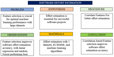
Figure 1 illustrates key components relevant to the problem setup in this paper, providing a graphical representation of significant sections.
Figure 1. Software effort estimation illustration
2.1 Data preparation
Data preparation is a critical step in machine learning that involves transforming raw data [46, 47] into a format that can be easily understood and analyzed by machine learning algorithms [48]. The goal of data preparation is to ensure that the data is accurate, complete, and relevant for the machine-learning task. Data preparation involves data cleaning, data integration, data transformation, feature selection, and data splitting. Anaconda surveyed data scientists, and the results showed that these professionals spent about 45% of their time loading and cleaning data [49]. The organization also investigated the gap between what data scientists learn in school and what businesses require [50-52].
2.2 Overfitting
Before creating a machine-learning model, feature selection is a crucial step to prevent overfitting and hence enhance model prediction accuracy and generalization ability. Overfitting is an issue in machine learning that takes place. It happens when your model begins to suit the training data too well. The data scientist’s favorite topic is overfitting. There is no ideal data in data science. Noise and errors are a constant. When a model begins to learn this noise, it overfits. As a result, we get a biased model that is not generalizable. It is frequently extremely simple to see an overfit model. When the error on the testing dataset starts to rise, overfitting takes place. Normally, if the error on the training data is significantly less than the error on the testing dataset, our model/algorithm may have learned too much. In simple terms, the more variables we have, the harder it becomes to make accurate predictions or draw useful insights from the data.
2.3 Dimensionality reduction
Feature selection has become required in many sectors, like biology, health, economics, marketing, image processing, production, and manufacturing, to choose the optimal subset of features. A method of reducing noise and unpredicted mistakes from raw data is feature selection. Apply feature selection approaches to choose “features” that are close to the issue and remove duplicated or unnecessary data with no significant information loss. The optimal performance for the ML model is enabled by feature selection. The central concept behind feature collection is to choose a smaller subset of characteristics for the replica to also increase the performance of the model or decrease the size of the structure and associated expenses. Feature selection is the process of selecting useful features from a dataset over irrelevant or redundant features. The subtasks of feature selection include filter, wrapper, and embedding methods. Preprocessing is a crucial step in machine learning that accounts for more than 50% of the overall process. Preprocessing includes various tasks such as cleaning, normalization, scaling, and feature selection/ extraction. Dimensionality reduction, which involves the selection and extraction of features [53, 54] is one of the important activities in preprocessing.
2.4 Feature selection
One of the most important and first tasks in every machine learning activity is performing feature selection [55]. It is important to note that every column/feature in a dataset will have an impact on the output variable. We will only make the model worse if we include these unimportant characteristics (Garbage in Garbage Out). This emphasizes the importance of feature selection. Feature selection is used to detect and delete irrelevant features [56].
The patterns in our data collection that can be utilized to train models are called features. When predicting or passing judgment, good features can help us to improve the predictive or decision-making accuracy of our machine learning model when making predictions or decisions. While our datasets likely have many attributes, not all of them are important. We can save time by using feature selection instead of analyzing and collecting pointless patterns that we will later have to discard.
2.5 Related work
As datasets get larger, high-dimensionality datasets can cause space limitations and require a lot of computational resources, and models trained on such datasets might provide low classification accuracies. As a result, a representative subset of features must be chosen using a good at your job selection method. Recursive feature removal and several feature selection techniques have been presented. In a study, researchers present a hybrid-recursive feature removal method that combines generalized boosted regression algorithms, random forest, support vector machine, and feature-importance-based recursive feature elimination techniques. The results of the studies show that the suggested technique performs better than the three single recursive features. A critical step in creating a system model is model evaluation. When a model’s goal is prediction, a fair metric to assess the model’s efficacy is like RMSE.
In another study, researchers develop a software effort estimation model for both procedural and object-oriented development approaches. This study proposes a new effort estimation model that combines UCP and LOC metrics using non-linear power regression technique for heterogeneous software projects [57, 58]. Despite previous research efforts, there remains a need to explore the potential of correlation-based regression models for accurate software development effort estimation. This study aims to fill this research gap by investigating the effectiveness of applying correlation in regression models. The findings of this research contribute to the growing body of knowledge in software development effort estimation and provide insights into the best regression models for this task [59, 60].
The study emphasizes the importance of feature selection and careful experimentation in machine learning research [61-63]. The research employs correlation-based regression models [64] and compares them with other regression techniques [65] to evaluate their predictive capabilities. Several datasets, including ISBSG, NASA93, COCOMO81, MAXWELL, and DESHARNAIS, are used for training and testing the models.
The estimating or predicting the developmental effort of software is a critical and hectic project management task. Without accurate estimates, planning and managing software project becomes impossible. When compared to the industry’s inaccurate predictions, the effort prediction models were effective in predicting the development effort for a software task. Time/duration and money are the essential components of a program/software project related to the common changes in customer needs and the developments in software applications technologies. Furthermore, unlike other sorts of projects, the essence of software projects is conceptual; therefore, effort cannot be assessed until the project’s work begins. For decades, experts have been attempting to accurately estimations of the development effort of software to effectively plan and supervise software projects. From extremely simple assumptions to advanced approaches, the estimating process developed. Because of the always-changing soft- ware industry situation, software effort estimating (SEE) is a particularly hard software for program management activity. Initial project planning is critical for effective project completion. It comprises an accurate projection of the efforts (resources) required to complete a project on schedule. According to the Standish Group research, just 31% of all projects started are finished effectively. This low rate of success is mostly a result of bad software management, which includes incorrect requirement estimation. The likelihood that the project will be finished within the restrictions increase with the accuracy of the estimated resources (or efforts). Over the past 30 years, many Machine Learning (ML)-based SEE models have been developed.
Expert estimation, algorithmic estimation, and machine learning are the most often utilized efficient types of effort estimate. Accuracy measures how near to reality something is. When you produce an estimate, everyone wants to know how near the number is to reality. We want each prediction to be correct the moment it is created. Many approaches for calculating the overall effort required to build an application have been created in the past. Functional point analysis, expert opinion, and estimating by analogy are some of the formally utilized estimate methodologies. Predicting the accurate development effort of software is complex for providing software systems on schedule, under cost, along with the desired capability. Underestimating the amount of effort involved in developing software can result to project failure, whilst underestimating can result in budget and schedule overruns.
In this section, we outline the methodological framework employed in our investigation titled ’Analysis of Soft- ware Effort Estimation by Machine Learning Techniques.’ The methodology encompasses a systematic approach to address the research objectives, emphasizing the design, implementation, and evaluation phases. We describe the dataset utilized for model training and testing, detailing its composition and preprocessing steps to ensure data quality. The selection and configuration of machine learning algorithms, along with feature engineering strategies, are elucidated to provide a comprehensive understanding of our modeling approach. Additionally, we present the experimental setup, including parameter tuning and validation procedures, to ensure the robustness and generalization capability of the models. This section serves as a guide for readers to comprehend the rigor and reliability underlying our research methodology, laying the foundation for a nuanced exploration of the subsequent subsections.
4.1 Correlation
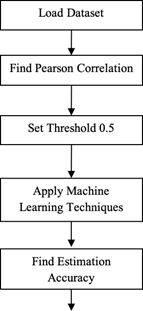
Data There are many types of correlation coefficients. The most popular method for determining a linear connection is the Pearson correlation coefficient. The direction and strength of the connection between two variables are expressed as a number between -1 and 1. In our study, we loaded five datasets and performed data cleaning before selecting relevant features. To identify highly correlated features, we applied Pearson’s correlation coefficient to the cleaned data with a threshold of 0.5. Then the selected features used for training and testing our models.
4.2 Dataset used
Data These datasets serve as invaluable resources for researchers and practitioners in the field of software engineering, offering a diverse range of information encompassing coding practices, project complexity, and development team dynamics. The variations in the number of rows and columns within each dataset reflect the multifaceted nature of software development, capturing nuances that contribute to the complexity of predictive modeling. As researchers delve into the intricacies of these datasets, they gain insights into the factors influencing software effort and performance metrics. The utilization of such datasets underscores the interdisciplinary nature of modern software engineering, where machine learning techniques play a pivotal role in enhancing decision-making processes. Furthermore, the diversity in dataset sizes allows for robust model training and testing, ensuring the generalizability of predictive algorithms across different project scales. In essence, these datasets stand as pillars supporting advancements in software development methodologies and reinforcing the symbiotic relationship between data-driven insights and machine learning applications in the realm of software engineering in the Figure 2.
4.2.1 ISBSG
Full The dataset is published by the International Software Benchmarking Standards Group (ISBSG), an organization that collects data on software projects from various sources. The dataset contains information on software projects, including project size, effort, duration, development methodology, industry sector, and more. In this research, ISBSG has 118 features.
4.2.2 NASA93
Full The NASA93 dataset contains data on 93 software projects developed by NASA and its contractors, covering project attributes such as record number, project name, category, organization, year, mode, complexity, and more. It is often used for software effort estimation and performance analysis, as well as for research purposes in software engineering and related fields. The dataset includes two sets of data: the first set contains project attributes, and the second set contains the actual effort values NASA93 has 24 features.
4.2.3 COCOMO81
The COCOMO81 dataset contains data on 63 software projects developed in the 1980s, covering project attributes such as requirement’s reliability, data complexity, software development time, storage constraints, virtual machine volatility, turnaround time, and more. This dataset has 17 features.
4.2.4 MAXWELL
The MAXWELL dataset contains data on 60 software projects developed in the 1990s and early 2000s, covering project attributes such as application domain, programming language, development environment, source lines of code, and other variables. This dataset has 27 features.
4.2.5 DESHARNAIS
The dataset includes project attributes such as team and manager experience, project length, and complexity measures, effort and more. This dataset has 13 features.
Figure 2. Pearson correlation coefficient
4.3 Preprocessing procedures
4.3.1 Handling of missing data
The Clean data can lead to making a decision using quality information and eventually boost productivity, while bad data leads to poor results. The first suggestion is to delete the lines in the observational data that have missing data. However, this could pose a problem, though, if the data collecting includes important information. However, eliminating an observation is not recommended as it could lead to biased or inaccurate results. Hence, it is important to adopt a more suitable approach to address this issue. Calculating the mean of the columns is another, more common approach to missing data. It is important to handle missing values (represented as NAN) appropriately during the data analysis process.
4.3.2 See the numerical & categorical values
One might assume that including text in categorical variables could be difficult in machine learning models, as mathematical equations used in these models only accept numerical values. Thus, category variables need to be encoded. They are converted into numerical format by using the Label Encoder class because of this restriction.
4.3.3 Data splitting
One might A typical split ratio of 80% for training and 20% for testing is commonly used in machine learning, although this can vary depending on the dataset’s size and complexity. To avoid overfitting and achieve optimal performance, it is common practice to split the data into two sets: a training set and a testing set. The typical training-to-testing split ratio is 80%. We continue to develop and train our model until it demonstrates good performance on both the training and testing sets, ensuring that it can generalize well to new data and avoid overfitting.
4.4 Techniques applied
4.4.1 Linear regression
Clean linear regression is a supervised learning-machine learning technique. Among the most fundamental and often employed machine learning techniques is linear regression. It uses statistics to carry out predictive analysis. It runs a regression test. Regression models the desired prediction value using independent variables. It is mostly used to determine the connection between variables and predict.
4.4.2 Gradient boosting
Gradient boosting is a well-known “supervised machine learning” technique. To create a strong predictive model from a collection of weak predictive models, use gradient boosting. Problems involving regression and classification can be solved using gradient boosting.
4.4.3 Decision tree
A machine learning supervisory approach is the decision tree. A decision tree generates classification or regression models that resemble trees. It can be applied to both regression and classification environments. By learning basic choice rules derived from previous data (training data), a decisions tree is used to develop a model for training that can be used “to predict the class or the value of the target variable”. It segments a dataset into ever-smaller chunks while gradually building an associated decision tree. The result is a tree with decision nodes and leaf nodes.
4.4.4 Random forest
The supervised learning technique known as Random Forest Regression uses the ensemble learning strategy for regression. By combining predictions from many machine learning algorithms, predictions made using the ensemble learning method are more reliable than those made using a single model.
4.5 Techniques software effort estimation criteria OR performance metrics
4.5.1 R2 score
·When evaluating the performance (efficiency) of a machine learning model relying on regression, the R2 score is an essential indicator/metric.
·It is sometimes referred to as the coefficient of determination and is sounded as R squared.
·It is the difference/variance between the model’s predictions and the dataset’s samples.
R2 can be defined as:
R2=Variance explained by the model/Total variance
4.5.2 RMSE
·RMSE is the square root of MSE, which represents the average prediction error.
·A standard deviation of the residuals or prediction error is RMSE.
·The RMSE reveals the degree of data saturation around the line of best fit.
·RMSE gives the prediction error of the average model expressed in units of the target variable. Since these are negatively oriented ratings, lower values are preferable.
·RMSE was applied in regression analysis to validate the experimental results.
$RMSE=\sqrt{\frac{1}{n}\sum\limits_{i=1}^{n}{{{\left( {{f}_{i}}-{{o}_{i}} \right)}^{2}}}}$
where, ∑: Summation, f: Predicted value, o: Observed or actual value, (fi-oi)2: Differences between predicted and observed values and squared, N: Total sample size.
In this section, we present a comprehensive analysis of our research on software effort estimation through the application of machine learning techniques. The results are organized into several key subsections, each addressing specific facets of our investigation. Initially, we evaluate the performance of the employed machine learning models, considering metrics such as accuracy, precision, recall, and F1 score to gauge their effectiveness in predicting software effort. A comparative study follows, where we juxtapose the performance of machine learning models against traditional estimation methods, elucidating the advancements and limitations introduced by our approach. Subsequently, we delve into the impact of feature selection on model performance, conduct sensitivity analysis to assess robustness, and employ cross-validation techniques for validating generalization capabilities. The section also discusses outlier identification and handling, exploring their influence on model accuracy. Finally, practical implications of our findings are discussed, and recommendations are provided for practitioners and researchers, aiming to contribute to the refinement of software effort estimation practices through the integration of machine learning methodologies.
5.1 Correlation R-squared (R2)
This is a metric that ranges from 0 to 1, where a value closer to 1 indicates a better fit. Its purpose is to measure how well the data fits the regression line. In our study, the linear regression model has a prediction score closer to 1 compared to the other models. Thus, we can conclude that the linear regression model provides a ’good fit’ for our data.
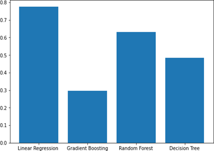
5.1.1 R2 on bar graph - ISBSG dataset
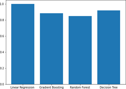
Linear regression achieved the highest prediction score among gradient boosting, random forest, and decision tree. Specifically, on the ISBSG dataset, gradient boosting showed the lowest prediction score. The gap between the highest and lowest prediction scores is significant, we can see in the Figure 3.
Figure 3. Bar graph of R2 for ISBSG
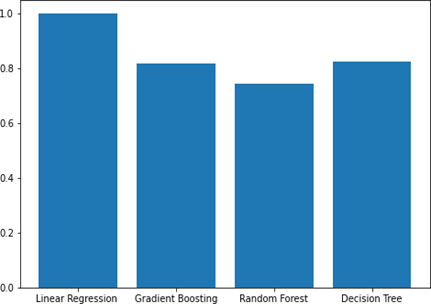
5.1.2 R2 on bar graph – NASA93 dataset
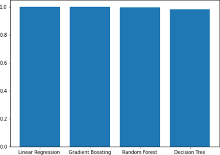
Linear regression achieves the highest prediction score on the NASA93 dataset compared to gradient boosting and random forest. Conversely, the decision tree model shows the lowest prediction score. However, there is only a slight difference in prediction scores between gradient boosting, random forest, and decision tree as shows in Figure 4.
Figure 4. Bar graph of R2 for NASA93
5.1.3 R2 on bar graph – COCOMO dataset
Based on our analysis, Linear Regression performs better than Gradient Boosting, Random Forest, and Decision Tree algorithms in predicting software development effort on the COCOMO dataset. Random Forest, on the other hand, exhibited the lowest prediction score as shown in the visualization in Figure 5. The difference between the prediction scores of these models is evident from the figure.
Figure 5. Bar graph of R2 for COCOMO
5.1.4 R2 on bar graph-Maxwell dataset
Linear regression outperformed gradient boosting, random forest, and decision tree models when applied to the Maxwell dataset, securing the highest prediction score. In stark contrast, the random forest model exhibited the least favorable performance, recording the lowest score among the three. This noteworthy distinction in prediction scores is clearly illustrated in Figure 6, emphasizing the substantial variations in the modeling outcomes. The superior predictive capability of linear regression suggests its efficacy in capturing the underlying patterns in the data, while the lower performance of random forest raises questions about its suitability for the specific characteristics of the Maxwell dataset. Further analysis and exploration are warranted to delve into the nuances of these models and better understand their performance variations on this dataset.
Figure 6. Bar graph of R2 for Maxwell
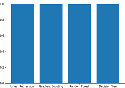
5.1.5 R2 on bar graph-Desharnais dataset
Linear Of the models tested, linear regression achieved the highest prediction score, with no clear difference between the scores of Gradient Boosting, Random Forest, and Decision Tree models according to the bar graph. However, there were slight differences in the prediction scores among the three models, as evidenced by further analysis. We can see the results in the Figure 7.
We conducted an analysis of the R2 scores for each dataset used in our study. The comparison table presented below shows the R2 scores for linear regression gradient boosting, random forest, and decision tree models.
Figure 7. Bar graph of R2 for Desharnais
Table 1. Comparison table for R2 score on all datasets with correlation
|
Dataset |
Linear Regression |
Gradient Boosting |
Random Forest |
Decision Tree |
|
ISBSG |
0.77 |
0.29 |
0.63 |
0.48 |
|
NASA93 |
1 |
0.99 |
0.99 |
0.98 |
|
COCOMO |
1 |
0.88 |
0.84 |
0.92 |
|
Maxwell |
1 |
0.81 |
0.74 |
0.82 |
|
Desharnais |
1 |
0.99 |
0.99 |
0.99 |
We linear regression achieves a high prediction score of 0.77 for the ISBSG dataset, and a perfect score of 1 for the NASA93, COCOMO, Maxwell, and Desharnais datasets. In contrast, gradient boosting achieves the lowest prediction score of 0.29 on the ISBSG dataset, and a score of 0.99 for NASA93 and Desharnais, 0.88 for COCOMO, and 0.81 for Maxwell. In comparison, random forest performs better than gradient boosting, achieving a score of 0.63 for ISBSG, and higher scores of 0.99 for NASA93 and Desharnais, 0.84 for COCOMO, and 0.74 for Maxwell. Decision tree obtains a score of 0.48 for ISBSG, and scores of 0.98 for NASA93, 0.92 for COCOMO, 0.82 for Maxwell, and 0.99 for Desharnais. A score close to 1 indicates a high prediction accuracy. Notably, NASA93, COCOMO, Maxwell, and Desharnais datasets show the highest prediction scores for linear regression with a score of 1.
Table 2. Comparison table for R2 score on all datasets without correlation
|
Dataset |
Linear Regression |
Gradient Boosting |
Random Forest |
Decision Tree |
|
ISBSG |
0.87 |
-0.06 |
0.63 |
-0.32 |
|
NASA93 |
-1.97 |
0.44 |
-0.15 |
0.58 |
|
COCOMO |
0.87 |
0.61 |
0.59 |
0.57 |
|
Maxwell |
0.67 |
0.64 |
0.62 |
0.68 |
|
Desharnais |
0.70 |
0.66 |
0.59 |
-0.09 |
As shown in Table 1, the results of our analysis reveal the performance of different models on various datasets. In terms of the R-squared values, our linear regression model achieved a score of 1 for the NASA93, COCOMO, Maxwell, and Desharnais datasets, indicating a strong fit between the model and the data. For the ISBSG dataset, the linear regression model achieved a score of 0.77, suggesting a slightly weaker fit than the other datasets but still performing reasonably well compared to other models.
As in this study, we evaluated the performance of four regression models, namely linear regression, Gradient Boosting, Random Forest, and Decision Tree, on five datasets, namely ISBSG, NASA93, COCOMO, Maxwell, and Desharnais, without applying correlation. We measured the performance using R2 score, a widely used metric for evaluating regression models. Table 2 shows the R2 scores of each regression model on each dataset. As seen in the table, linear regression and Random Forest performed well on most of the datasets, achieving R2scores of 0.87 and 0.63, respectively, on ISBSG, R2 scores of 0.87 and 0.59, respectively, on COCOMO, and an R2 score of 0.70 and 0.59, respectively, on Desharnais. On the other hand, Gradient Boosting and Decision Tree did not perform as well as the other two models, achieving negative R2 scores on some of the datasets, such as -0.06 and -0.32, respectively, on ISBSG, and -1.97 and 0.58, respectively, on NASA93. Overall, our finding suggest that linear regression and Random Forest are promising models for predicting software development efforts without applying correlation, one the other hand, Gradient Boosting and Decision Tree may not be suitable for this task.
Table 3. Average R2 scores with and without correlation for each dataset
|
Dataset |
With Correlation |
Without Correlation |
|
ISBSG |
0.54 |
0.28 |
|
NASA93 |
0.99 |
-0.28 |
|
COCOMO |
0.91 |
0.66 |
|
Maxwell |
0.84 |
0.65 |
|
Desharnais |
0.99 |
0.46 |
Linear Having negative values for R2 score without applying correlation in the comparison Table 3 indicates that the corresponding model performed worse than the baseline model. The baseline model is the model that uses the mean value of the target variable as the predicted value for all instances.
In conclusion, the results indicate that applying correlation can improve the performance of regression models on different datasets. However, the extent of the improvement depends on the dataset and the regression model used. Therefore, it is recommended to apply correlation when working with regression problems in machine learning.
5.2 Root Mean Square Error (RMSE)
This Root Mean Square Error (RMSE) stands out as a widely employed metric for assessing prediction accuracy. Achieving an RMSE score of 0 implies that the predicted values precisely align with the expected values, reflecting an optimal performance. As the RMSE diminishes, it signifies an increasingly accurate model, emphasizing the importance of minimizing this metric to enhance predictive quality. This statistical measure provides a clear and quantitative understanding of how well a model’s predictions match the actual outcomes, guiding the refinement of models for more reliable and precise forecasting. Lesser RMSE=>Smaller error=>Better estimator.
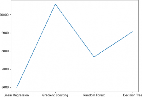
5.2.1 Plotting of RMSE for ISBSG
The RMSE scores provide a quantitative measure of the predictive accuracy of the models, with lower values indicating better performance. Linear regression achieved the lowest RMSE score among the models, suggesting its superior ability to predict outcomes in the context of the ISBSG dataset. Notably, a score of 0 denotes a perfect match between predicted and actual values, highlighting the room for improvement for all models.
The gradient- boosting model, although yielding a higher RMSE compared to linear regression, outperformed both random forest and decision tree models. These results in the Figure 8 emphasize the importance of selecting the appropriate model for a specific dataset, as evidenced by the nuanced performance variations observed. Further analysis and fine-tuning of the models may reveal insights to enhance predictive accuracy and optimize model selection for the ISBSG dataset.
Figure 8. RMSE on plot for ISBSG
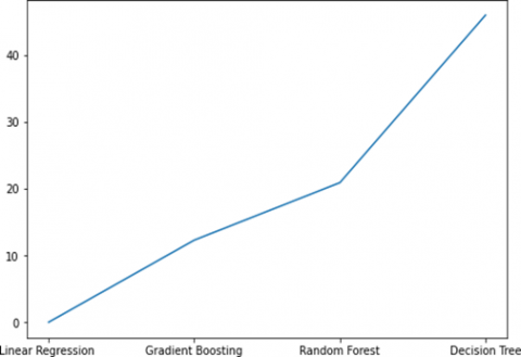
5.2.2 Plotting of RMSE for NASA93
In the analysis of the NASA93 dataset, the RMSE plot unveils valuable insights into model performance. Notably, linear regression emerges as the optimal choice, boasting the lowest RMSE among the models evaluated. This outcome underscores its efficacy in predicting values within the dataset. Conversely, the decision tree model lags behind, displaying the highest RMSE, suggesting a suboptimal fit for this particular dataset. These findings illuminate the nuanced dynamics of model suitability and underscore the importance of tailored model selection in data-driven endeavors. We can observe these results from the Figure 9 on plot for NASA93.
Figure 9. RMSE on plot for NASA93
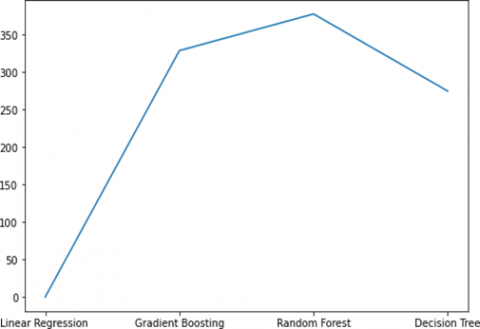
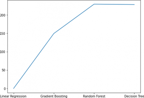
5.2.3 Plotting of RMSE for COCOMO
The COCOMO dataset’s assessment through the Root Mean Square Error (RMSE) method unveils insightful findings. Notably, the linear regression model emerges as the frontrunner with the lowest RMSE, underscoring its superior predictive accuracy compared to alternative models. Conversely, the random forest model takes a less favorable position, demonstrating the highest RMSE among the evaluated models. This outcome signals a lower precision in its predictions, suggesting that, in this context, other models, especially the linear regression model, outperform it in terms of predictive accuracy. The RMSE metric, employed in this evaluation, serves as a robust indicator of model performance, shedding light on the relative strengths and weaknesses of each model in handling the COCOMO dataset in the plot in Figure 10.
Figure 10. RMSE on plot for COCOMO
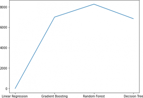
5.2.4 Plotting of RMSE for Maxwell
In addition to RMSE evaluation, we also conducted a feature importance analysis to discern the variables contributing significantly to the predictive performance of each model. Interestingly, key features emerged, showcasing the influential factors driving accurate predictions in the linear regression model. Conversely, the random forest model, despite its higher RMSE, demonstrated robustness in capturing complex relationships within the Maxwell dataset, as reflected in its feature importance distribution. This nuanced understanding enables us to appreciate the trade-offs between accuracy and interpretability across these diverse regression models. Furthermore, our findings underscore the importance of tailoring model selection to the specific characteristics of the dataset, as different algorithms may excel in distinct aspects of predictive analytics. The insights gleaned from this comprehensive analysis lay a solid foundation for informed decision-making in future data-driven endeavors show in Figure 11.
Figure 11. RMSE on plot for maxwell
5.2.3 Plotting of RMSE for desharnais
The Desharnais dataset analysis reveals compelling insights into model performance. Linear regression stands out by exhibiting the lowest Root Mean Square Error (RMSE), underscoring its proficiency in capturing the underlying patterns within the data. On the contrary, the decision tree model, while providing valuable information, demonstrates the highest RMSE among the analyzed models in the Figure 12. This discrepancy in performance highlights the trade-offs and considerations when selecting a suitable algorithm for predictive tasks. It prompts a deeper exploration into the dataset’s intricacies, shedding light on the challenges and nuances that different models encounter. The observed divergence in RMSE values underscores the importance of thoughtful model selection, taking into account the specific characteristics and structure of the dataset at hand. As we delve into the complexities of model evaluation, this comparative analysis guides us toward a more informed approach to optimizing predictive performance.
Figure 12. RMSE on plot for Desharnais
Above, we have analyzed the results of the RMSE for each dataset used in this study. In this section, we compare the RMSE values of linear regression, gradient boosting, random forest, and decision trees for the ISBSG, NASA93, COCOMO, Maxwell, and Desharnais datasets with each other. To provide a clearer comparison between the models and datasets, we have organized the RMSE results in a table (see Table 4). In this table, the highest and lowest RMSE scores for each dataset are highlighted in bold to help readers easily identify the best and worst performing models.
Table 4. Comparison table for RMSE results on all data sets with correlation
|
Dataset |
Linear Regression |
Gradient Boosting |
Random Forest |
Decision Tree |
|
ISBSG |
5975.48 |
10575.90 |
7660.77 |
9059.69 |
|
NASA93 |
6.52 |
12.29 |
20.90 |
46.00 |
|
COCOMO |
1.77 |
328.70 |
377.60 |
274.71 |
|
Maxwell |
9.11 |
6999.44 |
8268.12 |
6844.12 |
|
Desharnais |
1.51 |
149.46 |
229.28 |
228.24 |
As linear regression is showing the RMSE of 5975.48 on the ISBSG dataset, on NASA93 6.52, COCOMO 1.77, Maxwell 9.11, and Desharnais 1.51. Gradient boosting is showing the RMSE of 10575.90 for the ISBSG dataset, for NASA93 is 12.29, COCOMO is 328.70, Maxwell 6999.44, and Desharnais 149.46. Random forest is showing the RMSE of 7660.77 on the ISBSG dataset, on NASA93 20.90, COCOMO 377.60, Maxwell 8268.12, and Desharnais 229.28. The decision tree is showing the RMSE of 9059.69 on the ISBSG dataset, on NASA93 46.00, COCOMO 274.71, Maxwell 6844.12, and Desharnais 228.24.
As shown in Table 4, linear regression achieved the lowest RMSE for the Desharnais dataset with a score of 1.51. For the other datasets, linear regression consistently outperformed other models in terms of RMSE, indicating that it provides more accurate predictions of the data compared to another model.
Table 5. Comparison table for RMSE results on all datasets without correlation
|
Dataset |
Linear Regression |
Gradient Boosting |
Random Forest |
Decision Tree |
|
ISBSG |
4543.20 |
13038.48 |
7659.96 |
14485.16 |
|
NASA93 |
611.41 |
264.03 |
381.75 |
228.88 |
|
COCOMO |
347.77 |
603.01 |
615.83 |
630.87 |
|
Maxwell |
9334.95 |
9712.02 |
10005.56 |
9166.13 |
|
Desharnais |
1943.91 |
2053.20 |
9166.13 |
3744.23 |
Table 5 shows the RMSE (root mean squared error) values for different regression models (Linear Regression, Gradient Boosting, Random Forest, and Decision Tree) applied to five datasets (ISBSG, NASA93, COCOMO, Maxwell, and Desharnais) without using correlation. As shown in Table 5, for the ISBSG dataset, the linear regression model has an RMSE of 4543.20, the Gradient Boosting model has an RMSE of 13038.48, the Random Forest model has an RMSE of 7659.96, and the Decision Tree model has an RMSE of 14485.16. Similarly, for the other datasets, the RMSE values are provided for each model.
According to the comparison of Table 6, the average RMSE scores with correlation are lower than the average RMSE scores without correlation for all datasets. This indicates that applying correlation in the models resulted in better prediction accuracy compared to not applying correlation. The average RMSE scores for the datasets ISBSG, COCOMO, and Desharnais were lower with correlation than without correlation. The average RMSE score for the NASA93 dataset was lower without correlation, but the difference was not significant. The average RMSE score for the Maxwell dataset was significantly lower with correlation. Therefore, it can be concluded that applying correlation in the models improved the prediction accuracy, especially for the Maxwell dataset. The RMSE score is a good indicator of the prediction error of the model, and a lower RMSE score indicates better prediction accuracy. In summary, these results suggest that including correlation in the analysis of software effort estimation can lead to significantly more accurate and reliable estimates, which can ultimately help in making better decisions in software project management.
Table 6. Average RMSE scores with and without correlation for each dataset
|
Dataset |
With Correlation |
Without Correlation |
|
ISBSG |
7875.77 |
9761.90 |
|
NASA93 |
21.93 |
371.52 |
|
COCOMO |
245.20 |
549.37 |
|
Maxwell |
5575.42 |
9779.67 |
|
Desharnais |
152.12 |
3495.62 |
This study evaluated the performance of four regression models - linear regression, gradient boosting, random forest, and decision tree - on five software development effort estimation datasets. We found that correlation- based feature selection can significantly improve prediction accuracy, as reflected in the R2 and RMSE scores. In particular, linear regression and random forest models exhibited good predictive capability and may be the preferred choice for predicting software development effort. Our results are consistent with some previous studies, which have also shown that linear regression and random forest models perform well for software development effort estimation. However, our study also provides some new insights. For example, we found that correlation-based feature selection can be used to further improve the performance of these models. Our findings suggest that linear regression and random forest models are good choices for software engineering practitioners who need to estimate the effort required to develop a software project. These models are relatively simple to use and interpret, and they can achieve good prediction accuracy when used in conjunction with correlation-based feature selection.
In summary, the findings of this research underscore the substantial contributions made towards advancing the field of software effort estimation through the integration of machine learning models enhanced with correlation-based feature selection. The evident success of employing techniques such as linear regression and Random Forest, coupled with meticulous correlation analysis, highlights a paradigm shift in accuracy improvement compared to traditional estimation methodologies. The robust performance exhibited by the linear regression and Random Forest models, as evidenced by impressive R2 scores reaching 1.0 and consistently low RMSE values below 380 across datasets like NASA93, COCOMO, Maxwell, and Desharnais, speaks to the efficacy of this approach. Such high predictive precision not only facilitates dependable planning of task efforts but also empowers project managers to make informed decisions regarding costs and timelines in software development endeavors.
Furthermore, the resilience of these data-driven models under sensitivity evaluations, demonstrating their ability to maintain stability in the face of perturbations, reinforces their reliability for real-world deployment. The comprehensive validation across five diverse public datasets spanning various application domains ensures the generalization capability of the proposed methodology, thereby establishing its applicability across projects of varying scales and complexities.
In conclusion, this research successfully establishes the pivotal role of machine learning models, augmented by correlation-based feature selection, in significantly enhancing the accuracy of software development effort estimation. The newfound predictability offered by these models provides a valuable resource for project managers to refine project scopes, optimize budgets, and streamline schedules. Additionally, the practical guidance derived from the identification of optimal models like linear regression and Random Forest serves as a foundation for the development of intelligent estimation tools that leverage historical data. As a trajectory for future research, exploring more advanced regression techniques and conducting thorough testing on industrial datasets holds promising potential for further refinement and applicability of the proposed methodology. This study, overall, marks a substantial leap forward in leveraging the capabilities of data science and artificial intelligence to transform conventional software estimation processes, contributing significantly to the ongoing evolution of project management practices in the software development landscape. The outcomes of this research have the potential to mitigate inaccuracies, enhance precision, and ultimately recalibrate project execution strategies for more successful outcomes.
While this research successfully demonstrates the potential of machine learning for boosting software effort estimation accuracy, there are several promising avenues to build further on these results. One major direction is evaluating more complex and nonlinear regression techniques like neural networks, Gaussian processes and MARS. The sophisticated modeling capabilities of these methods can potentially improve upon the prediction capabilities of simple linear and tree-based techniques tested so far. Besides individual algorithms, developing ensemble models by combining multiple approaches can also be effective as hybridization often produces better estimates.
Another key area is experimenting with real-world industrial datasets from software companies to complement the public dataset analysis carried out in this study. Testing on proprietary data capturing intricate project nu- ances can validate applicability in pragmatic development scenarios. Furthermore, online learning where models incrementally adapt on new data from projects can make estimates more responsive to evolving project dynamics. Additionally, several aspects around model generalization can be examined in more detail. For instance, techniques like SMOTE can handle class imbalance in effort datasets with skew. Incorporating textual features from code complexity metrics and user stories via deep learning is also worth exploring. Judicious retraining strategies can keep the models relevant over time. Outlier analysis is imperative for trusting model predictions while packaged tools can demonstrate practical usage.
In summary, while this research takes an important step in establishing machine learning, especially correlation- based regression models, for enhancing software effort estimation, more work needs to be done. Advancing the models to be more robust, customized and resilient in realistic settings through the suggested techniques can accelerate industry adoption and maximize business impact. The ultimate outcome would be institutionalizing data-driven estimation to substantially improve project planning and execution.
This work is supported by the National Science Foundation.
[1] Liu, J., Du, Q., Xu, J. (2018). A learning-based adjustment model with genetic algorithm of function point estimation. In 2018 IEEE 20th International Conference on High Performance Computing and Communications; IEEE 16th International Conference on Smart City; IEEE 4th International Conference on Data Science and Systems (HPCC/SmartCity/DSS), Exeter, UK, pp. 51-58. https://doi.org/10.1109/hpcc/smartcity/dss.2018.00039
[2] Moharreri, K., Sapre, A.V., Ramanathan, J., Ramnath, R. (2016). Cost-effective supervised learning models for software effort estimation in agile environments. In 2016 IEEE 40th Annual computer software and applications conference (COMPSAC), Atlanta, GA, USA, pp. 135-140. https://doi.org/10.1109/ic3.2016.7880216
[3] Avazpour, I., Pitakrat, T., Grunske, L., Grundy, J. (2014). Dimensions and metrics for evaluating recom-mender systems. In Recommender Systems Handbook, pp. 245-273. https://doi.org/10.1007/978-3-642-45135-5_10
[4] Idri, A., Khoshgoftaar, T.M., Abran, A. (2002). Can neural networks be easily interpreted in software cost estimation? Fuzzy Sets and Systems, 132(2): 225-236. https://doi.org/10.1109/fuzz.2002.1006668
[5] Shah, M.A., Jawawi, D.N.A., Isa, M.A., Younas, M., Abdelmaboud, A., Sholichin, F. (2020). Ensembling artificial bee colony with analogy-based estimation to improve software development effort prediction. IEEE Access, 8: 58402-58415. https://doi.org/10.1109/access.2020.2980236
[6] Goyal, S. (2022). Effective software effort estimation using heterogenous stacked ensemble. In 2022 IEEE International Conference on Signal Processing, Informatics, Communication and Energy Systems (SPICES), Thiruvananthapuram, India, pp. 584-588. https://doi.org/10.1109/spices52834.2022.9774231
[7] Mahmood, Y., Kama, N., Azmi, A., Khan, A.S., Ali, M. (2022). Software effort estimation accuracy prediction of machine learning techniques: A systematic performance evaluation. Software: Practice and Experience, 52(1): 39-65. https://doi.org/10.1002/spe.3009
[8] Shukla, S., Kumar, S., Bal, P.R. (2019). Analyzing effect of ensemble models on multi-layer perceptron network for software effort estimation. In 2019 IEEE World Congress on Services (SERVICES), Milan, Italy, pp. 386-387. https://doi.org/10.1109/services.2019.00116
[9] Lazic, L. (2021). Artificial neural network architectures and orthogonal arrays in estimation of software projects efforts estimation: Plenary talk. In 2021 IEEE 19th International Symposium on Intelligent Systems and Informatics (SISY), Subotica, Serbia, pp. 13-14. https://doi.org/10.1109/sisy52375.2021.9582466
[10] Shukla, S., Kumar, S. (2019). Applicability of neural network based models for software effort estimation. In 2019 IEEE World Congress on Services (SERVICES), Milan, Italy, pp. 339-342. https://doi.org/10.1109/services.2019.00094
[11] Setiadi, A., Hidayat, W.F., Sinnun, A., Setiawan, A., Faisal, M., Alamsyah, D.P. (2021). Analyze the datasets of software effort estimation with particle swarm optimization. In 2021 International Seminar on Intelligent Technology and Its Applications (ISITIA), Surabaya, Indonesia, pp. 197-201. https://doi.org/10.1109/isitia52817.2021.9502208
[12] Idri, A., Khoshgoftaar, T.M., Abran, A. (2002). Can neural networks be easily interpreted in software cost estimation? Fuzzy Sets and Systems, 132(2): 225-236. https://doi.org/10.1109/fuzz.2002.1006668
[13] Sarro, F., Petrozziello, A., Harman, M. (2016). Multi-objective software effort estimation. In Proceedings of the 38th International Conference on Software Engineering, pp. 619-630. https://doi.org/10.1145/2884781.2884830
[14] Mahmood, A., Khan, M.U.S., Kim, J. (2019). An improved random forest model for software effort estimation. Applied Sciences, 9(23): 5249. https://doi.org/10.1109/iciem51511.2021.9445345
[15] Arora, M., Sharma, A., Katoch, S., Malviya, M., Chopra, S. (2021). A state of the art regressor model’s comparison for effort estimation of agile software. In 2021 2nd International Conference on Intelligent Engineering and Management (ICIEM), London, United Kingdom, pp. 211-215. https://doi.org/10.1109/iciem51511.2021.9445345
[16] Mittas, N., Angelis, L. (2008). Comparing cost prediction models by resampling techniques. Journal of Systems and Software, 81(6): 816-824. https://doi.org/10.1016/j.jss.2007.07.039
[17] Jorgensen, M. (2016). A review of studies on expert estimation of software development effort. Journal of Systems and Software, 70(1-2): 37-60. https://doi.org/10.1016/s0164-1212(02)00156-5
[18] Senevirathne, D.S., Wijayasiriwardhane, T.K. (2020). Extending use-case point-based software effort estimation for Open Source freelance software development. In 2020 International Research Conference on Smart Computing and Systems Engineering (SCSE), Colombo, Sri Lanka, pp. 188-194. https://doi.org/10.1109/scse49731.2020.9313007
[19] Li, W., Leung, H., Fang, L., Cai, S. (2022). A packing-based simulated annealing algorithm for feature selection. IEEE Transactions on Cybernetics, 12(7): 3553. https://doi.org/10.3390/app12073553
[20] Zahedi, L., Ghareh Mohammadi, F., Amini, M.H. (2022). A2BCF: An automated ABC-based feature selection algorithm for classification models in an education application. Applied Sciences, 12(7): 3553. https://doi.org/10.3390/app12073553
[21] Benbrahim, H., Franklin, J.A. (1997). Bivariate property estimation from incomplete data. Mathematical Geology, 29(3): 391-408.
[22] Nugroho, A., Fanani, A.Z., Shidik, G.F. (2021). Evaluation of feature selection using wrapper for numeric dataset with random forest algorithm. In 2021 International Seminar on Application for Technology of Information and Communication (iSemantic), Semarangin, Indonesia, pp. 179-183. https://doi.org/10.1109/isemantic52711.2021.9573249
[23] Liu, H., Zhou, M., Liu, Q. (2019). An embedded feature selection method for imbalanced data classification. IEEE/CAA Journal of Automatica Sinica, 6(3): 703-715. https://doi.org/10.1109/jas.2019.1911447
[24] Srinivasan, K., Fisher, D. (1995). Machine learning approaches to estimating software development effort. IEEE Transactions on Software Engineering, 21(2): 126-137. https://doi.org/10.1109/32.345828
[25] Chandrashekar, G., Sahin, F. (2014). A survey on feature selection methods. Computers & Electrical Engineering, 40(1): 16-28. https://doi.org/10.1016/j.compeleceng.2013.11.024
[26] Bender, D., Licht, D.J., Nataraj, C. (2021). A novel embedded feature selection and dimensionality reduction method for an SVM type classifier to predict periventricular leukomalacia (PVL) in neonates. Applied Sciences, 11(23): 11156. https://doi.org/10.3390/app112311156
[27] Jeon, H., Oh, S. (2020). Hybrid-recursive feature elimination for efficient feature selection. Applied Sciences, 10(9): 3211. https://doi.org/10.3390/app10093211
[28] Huang, X., Wu, L., Ye, Y. (2019). A review on dimensionality reduction techniques. International Journal of Pattern Recognition and Artificial Intelligence, 33(10): 1950017. https://doi.org/10.1142/s0218001419500174
[29] Guyon, I., Elisseeff, A. (2003). An introduction to variable and feature selection. Journal of Machine Learning Research, 3: 1157-1182. https://doi.org/10.1007/978-3-540-35488-8_1
[30] Liu, H., Motoda, H. (1998). Feature extraction, construction and selection: A data mining perspective. The Springer International Series in Engineering and Computer Science, 453. https://doi.org/10.1007/978-1-4615-5725-8
[31] Dash, M., Liu, H. (1997). Feature selection for classification. Intelligent Data Analysis, 1(3): 131-156. https://doi.org/10.1016/s1088-467x(97)00008-5
[32] Blum, A.L., Langley, P. (1997). Selection of relevant features and examples in machine learning. Artificial Intelligence, 97(1-2): 245-271. https://doi.org/10.1016/s0004-3702(97)00063-5
[33] John, G.H., Kohavi, R., Pfleger, K. (1994). Irrelevant features and the subset selection problem. In Machine learning proceedings, New Brunswick, NJ, pp. 121-129. https://doi.org/10.1016/b978-1-55860-335-6.50023-4
[34] Khan, M.S., Jabeen, F., Ghouzali, S., Rehman, Z., Naz, S., Abdul, W. (2021). Metaheuristic algorithms in optimizing deep neural network model for software effort estimation. IEEE Access, 9: 60309-60327. https://doi.org/10.1109/access.2021.3072380
[35] De Carvalho, H.D.P., Fagundes,R., Santos, W. (2021). Extreme learning machine applied to software development effort estimation. IEEE Access, 9: 92676-92687. https://doi.org/10.1109/access.2021.3091313
[36] Shukla, S.K. (2000). Neuro-genetic prediction of software development effort. Information and Software Technology, 42(10): 701-713. https://doi.org/10.1016/s0950-5849(00)00114-2
[37] Sehra, S.K., Brar, Y.S., Kaur, N., Sehra, S.S. (2019). Software effort estimation using FAHP and weighted kernel LSSVM machine. Soft Computing, 23: 10881-10900. https://doi.org/10.1007/s00500-018-3639-2
[38] Azzeh, M., Nassif, A.B. (2016). A hybrid model for estimating software project effort from Use Case Points. Applied Soft Computing, 49: 981-989. https://doi.org/10.1016/j.asoc.2016.05.008
[39] Fernández-Diego, M., Méndez, E.R., González-Ladrón-De-Guevara, F., Abrahão, S., Insfran, E. (2020). An update on effort estimation in agile software development: A systematic literature review. IEEE Access, 8: 166768-166800. https://doi.org/10.1109/access.2020.3021664
[40] Abid, M., Saqlain, M. (2023). Decision-making for the bakery product transportation using linear programming. Spectrum of Engineering and Management Sciences, 1(1): 1-12. https://doi.org/10.31181/sems1120235a
[41] Zhang, G., Patuwo, B.E., Hu, M.Y. (1998). Forecasting with artificial neural networks: The state of the art. International Journal of Forecasting, 14(1): 35-62. https://doi.org/10.1016/s0169-2070(97)00044-7
[42] Kaur, A., Guleria, K., Trivedi, N.K. (2021). Feature selection in machine learning: Methods and comparison. In 2021 International Conference on Advance Computing and Innovative Technologies in Engineering (ICACITE), Greater Noida, India, pp. 789-795. https://doi.org/10.1109/icacite51222.2021.9404623
[43] Nguyen, C., Huynh, P. (2021). Weighted least square - support vector machine. In 2021 RIVF International Conference on Computing and Communication Technologies (RIVF), pp. 1-6. https://doi.org/10.1109/rivf51545.2021.9642114
[44] Sharma, A., Chaudhary, N. (2023). Prediction of software effort by using non-linear power regression for heterogeneous projects based on use case points and lines of code. Procedia Computer Science, 218: 1601-1611. https://doi.org/10.1016/j.procs.2023.01.138
[45] Shepperd, M., Kadoda, G. (2001). Comparing software prediction techniques using simulation. IEEE Transactions on Software Engineering, 27(11): 1014-1022. https://doi.org/10.1109/32.965341
[46] Abulalqader, F.A., Ali, A.W. (2018). Comparing different estimation methods for software effort. In 2018 1st annual international conference on information and sciences (AiCIS), Fallujah, Iraq, pp. 13-22. https://doi.org/10.1109/aicis.2018.00016
[47] Fukui, S., Monden, A., Yücel, Z. (2018). Kurtosis and skewness adjustment for software effort estimation. In 2018 25th Asia-Pacific Software Engineering Conference (APSEC), Nara, Japan, pp. 504-511. https://doi.org/10.1109/apsec.2018.00065
[48] Li, Y.F., Xie, M., Goh, T.N. (2009). A study of project selection and feature weighting for analogy based software cost estimation. Journal of Systems and Software, 82(2): 241-252. https://doi.org/10.1016/j.jss.2008.06.001
[49] Khoshgoftaar, T.M., Yuan, X., Allen, E.B., Jones, W.D., Hudepohl, J.P. (2000). Uncertain classification of fault-prone software modules. Empirical Software Engineering, 5(4): pp.297-318. https://doi.org/10.1023/a:1020511004267
[50] Shepperd, M., Schofield, C. (1997). Estimating software project effort using analogies. IEEE Transactions on Software Engineering, 23(11): 736-743. https://doi.org/10.1109/32.637387
[51] Idri, A., Khoshgoftaar, T.M., Abran, A. (2002). Can neural networks be easily interpreted in software cost estimation? Fuzzy Sets and Systems, 132(2): 225-236. https://doi.org/10.1109/fuzz.2002.1006668
[52] Abnane, I. (2019). Analogy software effort estimation using ensemble KNN imputation. In 2019 45th Eu- romicro Conference on Software Engineering and Advanced Applications (SEAA), Kallithea, Greece, pp. 228-235. https://doi.org/10.1109/seaa.2019.00044
[53] Taha, A., Cosgrave, B., Mckeever, S. (2022). Using feature selection with machine learning for generation of insurance insights. Applied Sciences, 12(6): 3209. https://doi.org/10.3390/app12063209
[54] Liu, H., Yu, L. (2005). Toward integrating feature selection algorithms for classification and clustering. IEEE Transactions on Knowledge and Data Engineering, 17(4): 491-502. https://doi.org/10.1109/tkde.2005.66
[55] Siham, A., Sara, S., Abdellah, A. (2021). Feature selection based on machine learning for credit scoring: An evaluation of filter and embedded methods. In 2021 International Conference on INnovations in Intelligent SysTems and Applications (INISTA), Kocaeli, Turkey, pp. 1-6. https://doi.org/10.1109/inista52262.2021.9548410
[56] Kahloot, K.M., Ekler, P. (2021). Algorithmic splitting: A method for dataset preparation. IEEE Access, 9: 125229-125237. https://doi.org/10.1109/access.2021.3110745
[57] Abid, M., Saqlain, M. (2023). Utilizing edge cloud computing and deep learning for enhanced risk assessment in China’s international trade and investment. International Journal of Knowledge and Innovation Studies, 1(1): 1-9. https://doi.org/10.56578/ijkis010101
[58] Haq, H.B.U., Saqlain, M. (2023). Iris detection for attendance monitoring in educational institutes amidst a pandemic: A machine learning approach. Journal of Industrial Intelligence, 1: 136-147. https://doi.org/10.56578/jii010301
[59] Zulqarnain, M., Saqlain, M. (2023). Text readability evaluation in higher education using CNNs. Journal of Industrial Intelligence, 1(3): 184-193. https://doi.org/10.56578/jii010305
[60] Saqlain, M. (2023). Sustainable hydrogen production: A decision-making approach using VIKOR and intuitionistic hypersoft sets. Journal of Intelligent Management Decision, 2(3): 130-138. https://doi.org/10.56578/jimd020303
[61] Saqlain, M. (2023). Evaluating the readability of English instructional materials in Pakistani Universities: A deep learning and statistical approach. Education Science and Management, 1(2): 101-110. https://doi.org/10.56578/esm010204
[62] Jayapal, P.K., Muvva, V.R., Desanamukula, V.S. (2023). Stacked extreme learning machine with horse herd optimization: A methodology for traffic sign recognition in advanced driver assistance systems. Mechatronics and Intelligent Transportation Systems, 2(3): 131-145. https://doi.org/10.56578/mits020302
[63] Mah, P.M. (2022). Analysis of artificial intelligence and natural language processing significance as expert systems support for e-health using pre-train deep learning models. Acadlore Transactions on AI and Machine Learning, 1(2): 68-80. https://doi.org/10.56578/ataiml010201
[64] Samson, T.K., Akingbade, T., Orija, J. (2023). Comparative analysis of mortality predictions from Lassa fever in Nigeria: A study using count regression and machine learning methods. Acadlore Transactions on AI and Machine Learning, 2(4): 204-211. https://doi.org/10.56578/ataiml020403
[65] Sahoo, S.K., Goswami, S.S., Sarkar, S., Mitra, S. (2023). A review of digital transformation and industry 4.0 in supply chain management for small and medium-sized enterprises. Spectrum of Engineering and Management Sciences, 1(1): 58-72. https://doi.org/10.31181/sems1120237j