K.V.B. Saraswathi Devi*![]() | Muktevi Srivenkatesh
| Muktevi Srivenkatesh![]()
© 2023 IIETA. This article is published by IIETA and is licensed under the CC BY 4.0 license (http://creativecommons.org/licenses/by/4.0/).
OPEN ACCESS
The increasing adoption of solar power as a renewable and eco-friendly energy source necessitates precise forecasting of solar power generation. Accurate predictions are crucial for effective grid management and the seamless integration of renewable energy into the power grid. This study proposes a novel hybrid meta-heuristic optimization framework, empowered by an ensemble deep learning model, to enhance the accuracy of solar power generation forecasting. The proposed methodology comprises several methodical phases: data pre-processing, feature extraction, feature selection, and deep learning-based forecasting. Initially, the collected raw data undergo a pre-processing stage involving data cleaning and standardization via the z-score method. Subsequent feature extraction transforms the pre-processed data into a reduced set of representative features, leveraging Linear Discriminant Analysis (LDA), measures of central tendency (Weighted arithmetic mean, Winsorized mean, standard deviation), statistical dispersion (Interquartile range (IQR), Median absolute deviation (MAD)), and Information Theoretic measures (Mutual Information and Information Gain). The optimal features are then selected through a newly proposed hybrid optimization approach, the Gorilla Customized Teaching Learning-Based Optimization (GC-TLBO) Algorithm, an innovative combination of the Artificial Gorilla Troops Optimizer (GTO) and the Teaching-Learning-Based Optimization (TLBO). Solar power forecasting is accomplished using a novel ensembled deep learning model, which integrates optimized Recurrent Neural Network (O-RNN) with a Deep Belief Network (DBN) and a Deep Convolutional Neural Network (DCNN). The final outcome is derived from the O-RNN, which inputs the results from the DBN and DCNN, respectively. The DBN and DCNN are trained using the optimal features derived from the GC-TLBO, while the weights of the RNN are fine-tuned using the same algorithm. The proposed model was implemented in Python (Google Colab), and its performance was evaluated using several metrics: Normalized Mean Square Error (NMSE), Mean Squared Relative Error (MSRE), Mean Squared Error (MSE), Mean Absolute Percentage Error (MAPE), and Root Mean Squared Error (RMSE). The results demonstrate that the proposed model outperforms existing models, offering superior forecasting performance.
solar power generation forecasting, teaching-learning based optimization and artificial gorilla troops optimizer, DCNN, O-RNN, deep belief network, convolutional neural network, gorilla customized teaching learning-based optimization
1.1 Background
The forecasting of solar power generation, a process integral to the optimization of the electrical grid, the financial assessment of solar projects, and the management of power supply and demand, necessitates the prediction of future electricity output of a solar power plant. Such forecasting can be accomplished through a variety of methods, including statistical models, Machine Learning (ML), and physical models incorporating solar radiation, temperature, and cloud coverage factors. Accurate forecasts are essential for guaranteeing a consistent and stable power supply derived from solar energy.
The field has seen a variety of approaches: a noteworthy two-stage approach normalizes renewable energy using the clear sky model method, followed by the implementation of adaptive linear time series models [1]. The importance of precise Photovoltaic (PV) power forecasting has been underscored as a crucial component in power system management, facilitating the secure and economical integration of PVs into the smart grid [2]. A classification of forecasting techniques has been proposed, dividing them into competitive ensemble forecasting and collaborative group forecasting [3]. The systematic classification of various categories of solar energy prediction frameworks, optimizers, and methods, known as taxonomy, is based on their similarities and differences [4].
Improvements in solar power forecasting have mitigated the impact of solar power's unpredictability on large-scale power system operations, resulting in reduced ramping costs for producers, start and shut-down costs, and solar power curtailment [5]. A novel spatial-temporal forecasting technique based on the vector auto regression framework has been proposed, incorporating solar generation data collected from smart meters and distribution transformer controllers [6]. A universally applicable and value-based set of metrics for solar forecasting has been proposed for a broad range of scenarios [7]. The analog ensemble technique has been employed for hourly-resolution daily regional PV power forecasting, utilizing open weather forecast and power measurement data [8].
Efforts to enhance forecasting efficiency have leveraged significant weather variables derived from PV analytical modeling [9], and the potential use of Gradient Boosted Regression Trees (GBRT) for predicting solar energy production in a multi-site framework has been explored [10]. To address the challenges posed by the volatile and discontinuous nature of wind power, an optimal decomposition approach known as EEMD has been utilized [11]. Certain probabilistic forecasting models have applied the Bayesian bootstrap to produce sample bootstrap distributions [12]. The Particle Swarm Optimization (PSO) has been recommended for precise forecasting of PV [13], and an ensemble neural network model for forecasting that includes SVM, BP neural network, and ELM has been proposed [14]. A simplified Long Short-Term Memory (LSTM) algorithm has been employed for forecasting solar energy generation one day in advance, built on the ML methodology framework [15].
1.2 Problem statement
Table 1 shows the solar power forecasting by profuse authors.
Table 1. Reviews in forecasting of solar power
|
S. No. |
Methodology |
Aim/Objective |
Disadvantages |
|
1. |
Swarm optimized RBF [16] Neural Network |
For enhance RBF Neural Network parameters using Swarm Intelligence algorithms in order to more accurately and robustly predict solar power generation. |
Computational complexity and costly |
|
2. |
Cluster Analysis and Ensemble model |
to increase forecast accuracy by grouping the data into homogeneous clusters (cluster analysis) and combining the results from various individual models (ensemble model) to create a final forecast. |
Sensitivity to outliers and subjectivity, increased complexity, the potential for over fitting, and challenging results to interpret. |
|
3. |
LSTM [17, 18] |
to accurately forecast future solar power generation using historical data and knowledge of environmental factors. |
It may struggle with long-term data dependencies and be expensive computationally. For accurate forecasts to be generated, a significant amount of training data may also be needed. |
|
4. |
WRF |
to precisely forecast energy output in order to plan and optimise. |
Limited accuracy as a result of complex atmospheric conditions and solar radiation variability, causing an under- or overestimation of predicted power generation. |
|
5. |
Sky Image based Model |
capture and analyse real-time cloud cover and atmospheric conditions in order to precisely forecast solar power generation [19]. |
Expensive hardware and upkeep costs, potential restrictions on cloud detection and interpretation, and potential errors due to changing weather conditions. |
|
6. |
NWP [20] based model |
For estimating the volume of solar energy that a solar power plant will produce. |
High computational cost, possibility of model bias and error, reliance on high-quality input data, and limitations in forecasting regional weather patterns and extreme events. |
|
7. |
ARMA |
by incorporating moving average and autoregressive models into time series data modelling in order to take into account historical trends and error patterns. |
Its inability to comprehend intricate non-linear relationships and outside factors, which results in limitations in prediction accuracy and reliability. |
|
8. |
Time Delay Neural Network (TDNN) |
using multiple time delays and non-linear activation functions in the neural network architecture to capture complex non-linear relationships and handle large amounts of data. |
The need for a lot of training data and the high computational complexity, which makes training take a lot longer and could lead to overfitting if proper regularisation techniques are not used. |
|
9. |
CNN |
to utilise convolutional layers and pooling techniques to take advantage of local and spatial correlations in large datasets, improving prediction accuracy and robustness. |
Difficulty in modelling global relationships and capturing distant dependencies. |
|
10. |
EEMD |
improve forecasting accuracy and robustness by breaking down and analysing multi-scale and non-linear features in time series data on solar power generation. |
Its sensitivity to noise, the potential for over-fitting, the necessity of appropriate parameter selection, and the need for validating results to ensure meaningful decomposition. |
1.3 Objective and contribution
1.3.1 Objectives
To develop a precise forecasting model for solar power generation: The prime purpose of the proposed work is to establish a forecasting model that accurately predicts solar power generation. This is essential for useful grid management and integration of renewable energy sources into the power grid.
To leverage deep learning techniques for solar power forecasting: The proposed work aims to leverage the strengths of deep learning techniques, including RNN, DBN, and Deep convolutional neural network (DCNN), to develop a robust forecasting model.
To select optimal features for solar power forecasting: The proposed work aims to extract various features from pre-processed data and select the optimal features for improved forecasting accuracy. This is achieved through the use of the Gorilla Customized Teaching Learning-Based Optimization (GC-TLBO) Algorithm, which combines the strengths of the standard Artificial Gorilla Troops Optimizer (GTO) and Teaching-Learning-Based Optimization (TLBO).
To measure the achievement of the proposed model: The proposed work aims to evaluate the performance of the model developed by means of various performance metrics, including NMSE, MSRE, MSE, MAPE, and RMSE. The analysis will help to determine the effectiveness of the proposed approach and its potential for real-world implementation.
1.3.2 Contribution
Ensembled-deep-learning approach: The proposed work presents an ensembled-deep-learning approach to accurately forecast solar power generation. The approach uses a combination of optimized Recurrent Neural Network (O-RNN), deep belief network (DBN), and Deep convolutional neural network (DCNN) to leverage the strengths of each model and improve forecasting accuracy.
Hybrid optimization approach: The proposed work introduces a new hybrid optimization approach called Gorilla Customized Teaching Learning-Based Optimization (GC-TLBO) Algorithm. This approach combines the strengths of the standard Artificial Gorilla Troops Optimizer (GTO) and Teaching-Learning-Based Optimization (TLBO) to select the optimal features for solar power forecasting.
Feature selection: The proposed work also presents a comprehensive feature selection process that extracts various features from pre-processed data, including Linear Discriminant Analysis (LDA), central tendency (Weighted arithmetic mean, Winsorizedmean, standard deviation), Statistical dispersion (Interquartile range (IQR), Median absolute deviation (MAD)), Mutual Information, and Information Gain. The GC-TLBO Algorithm is then used to select the optimal features for improved forecasting accuracy.
2.1 Machine learning technique
In 2021, Liu et al. have proposed a simplified approach to time series forecasting used as an ML-based LSTM model for a day-ahead solar power forecast was suggested and used a less train data to achieve best forecasting results without sacrificing accuracy. Table 2 shows ML Review.
Table 2. ML review
|
Author |
Advantage |
Disadvantage |
|
Liu et al. [14] |
Record intra-hour ramping under various weather conditions. |
Multi-variate time series forecasting using LSTM is not developed. |
2.2 Deep learning in solar power forecasting
In 2022, Das et al. [21] have introduced the precise forecasting of PV output power, a model established on a PSO-optimized support vector regression (SVR) was recommended. Based on the most significant historical experimental data gathered from a real PV power plant, an SVR-based model was created. By applying the proposed model to three different PV systems, it is experimentally confirmed.
In 2021, Aslam et al. [22] have suggested to forecast a day's worth of PV power using a DL built on a two-stage attention technique over LSTM. To procure the ideal set of hyper-parameters for the suggested DL, the Bayesian optimization algorithm is also used.
In 2022, Elsaraiti and Merabet [23] have introduced a technique that used DL to forecast the short-term power output of PV power plants to achieve the aforementioned, a deep learning method based on LSTM algorithm was assessed with regard to its capacity to forecast solar power details. Table 3 shows Reviews of DL.
Table 3. Reviews of DL
|
Author |
Advantage |
Disadvantage |
|
Das et al. [21] |
Decreases the cost of computation |
The researchers might look into sophisticated feature engineering methods. |
|
Aslam et al. [22] |
Extremely effective at forecasting |
Future research could incorporate more pertinent data sources, like historical solar power generation data. |
|
Elsaraiti and Merabet [23] |
Enables more effective operation of photovoltaic power plants |
Does not offer trustworthy data that would allow photovoltaic power plants to operate more effectively. |
2.3 Meta heuristic optimizes for feature selection
In 2021, Moayedi and Mosavi [24] have proposed a unique metaheuristic method, electromagnetic field optimisation (EFO), for optimal Sir prediction. This algorithm has a substantial advantage over other existing techniques in terms of its fast convergence. The EFO manages a nonlinear problem using an ANN architecture.
In 2018, Ghadimi et al. [25] have used a hybrid prediction strategy that incorporates a novel feature selection procedure as well as a complicated forecast engine based on a new intelligent algorithm. The power load signal was initially cleansed using a feature selection to identify suitable candidates for use as input to the forecast engine. Table 4 shows Review of Meta-heuristic Optimization.
Table 4. Meta-heuristic optimization
|
Author |
Advantage |
Disadvantage |
|
Moayedi and Mosavi [24] |
Dependable approach to predicting solar irradiance. |
Comparisons between the EFO and other strong optimizers or the use of hybrid, ensemble, and deep machine learning techniques would be highly desirable. |
|
Ghadimi et al. [25] |
Two-stage forecasting system |
applications of forecasting that must be made quickly |
2.4 Ensemble models
In 2019, Pan and Tan [26] have introduced a brand-new ensemble model-based method for forecasting solar generation based on cluster analysis. The adoption of two popular strategies to increase prediction accuracy. To obtain a weather regime, researches first perform cluster analysis based on solar generation, which increases computing effectiveness and eliminates the challenge of choosing which weather variables to include in the clustering process. In 2021, Aslam et al. have suggested to forecast a day's worth of PV power using a DL built on a two-stage attention mechanism over LSTM. To achieve the ideal set of hyper-parameters for the suggested DL, the Bayesian optimization algorithm was also used.
In 2020, Sheng et al. [27] have introduced the majority of machine learning-based forecasts in use today use batch learning. The model's structure and parameters are typically no longer changed after the training is finished. The climate was dynamic and complex, though. A fixed model finds it challenging to adjust to the climatic traits of various regions or eras. Table 5 shows the reviews on Literature reviews by various authors.
Table 5. Reviews on ensemble model
|
Author |
Advantage |
Disadvantage |
|
Bendali et al. [17] |
Efficiency is good. |
Compared to other models, speed is less. |
|
Das et al. [21] |
Daily hourly forecasting. |
Effective feature extraction or selection has no effect on forecast performance. |
|
Aslam et al. [22] |
Assemble trustworthy prediction outcomes. |
The transfer learning task is not added to domain adaptive learning. |
3.1 Overview of the ensembled-deep-learning approach
In this research work, a novel deep learning based solar power forecast model is introduced. Figure 1 shows the architecture of the proposed model. The proposed model includes the following stages:
Figure 1. Architecture of the proposed model
Step 1: Pre-processing: The collected raw data is pre-processed across data cleaning and z-score based data standardization.
Step 2: Feature Extraction: Features such as Linear Discriminant Analysis (LDA), central tendency (Weighted arithmetic mean, Winsorized mean, standard deviation), Statistical dispersion (Interquartile range (IQR), Median absolute deviation (MAD)), Mutual Information and Information Gain, are extracted from the pre-processed data.
Step 3: Feature Fusion: Feature Extraction are fused together by concatenation.
Step 4: Feature Selection: The optimal features are selected using the new Gorilla Customized Teaching Learning-Based Optimization (GC-TLBO), which is a conceptual amalgamation of the standard Artificial Gorilla Troops Optimizer (GTO) and Teaching-Learning-Based Optimization (TLBO), respectively.
Step 5: Solar Power Forecasting: It is done through the new ensembled deep learning model, which includes the optimized Recurrent Neural Network (O-RNN) and deep belief network (DBN) and Deep convolutional neural network (DCNN). The DBN and DCNN are trained using the selected optimal features acquired with Gorilla Customized Teaching Learning-Based Optimization (GC-TLBO) Algorithm. The weight of Recurrent Neural Network (RNN) is fine-tuned using the new Gorilla Customized Teaching Learning-Based Optimization (GC-TLBO) Algorithm.
Step 6: Final Outcome: The final outcome is obtained from the optimized Recurrent Neural Network (O-RNN), which intakes the outcomes from DBN and DCNN, respectively.
3.2 Deep learning models for solar power forecasting
Deep learning models have shown great promise in solar power forecasting due to their capacity to handle non-linear correlations and occupy complex patterns in facts. This phase is shown in Figure 2.
Figure 2. Solar power forecasting phase
3.2.1 DBN
Figure 3. Architecture of DBN
An artificial neural network (ANN) with more than two layers between the input and output layers is called a deep neural network (DNN) shown in Figure 3. Although there are various kinds of neural networks, they all share the same building blocks: neurons, synapses, weights, biases, and functions. Also, that it is a probabilistic generative model, is made up of double-layered unsupervised learning networks called RBM and supervised learning networks called Back Propagation. Considering the qualities of the modules in the layer above, each layer's units in a DBN are independent.
A DBN with $n h$ layers can be described as a diagrammatic model. The joint distribution of the transparent layer $v u$ and the invisible layer $h n_{k b}$, for $k b=1: n h$ is circumscribed in Eq. (1).
$\begin{aligned} & p q\left(v u, h n_1, \ldots, h n_{n h}\right)=p q\left(v u \mid h n_1\right) \\ & \prod_{k b=1: w n-2} p q\left(h n_{k b} \mid h n_{k b+1}\right) p q\left(h n_{n h-1} \mid h n_{k b}\right)\end{aligned}$ (1)
DBN training is divided into two stages. Contrastive divergence (CD) algorithm is used to train the RBM of layer n in the first phase, and this layer-by-layer unattended, greedy learning calculation is a very efficient way to pre-train a DBN. First, the bottom distribution $p q\left(h n_1 \mid v u\right)$ is modelled from the higher-ranking RBM, and the obvious variables $v u$ are sampled by the posterior Distribution $\left(\mathrm{vu} \mid h n^1\right)$. Afterwards, the hidden variables $h n_1$ are patterned once more in a similar manner. $k b$ steps of alternating Gibbs sampling were continually carried out until an arbitrary equilibrium dispersion is attained. Then optimal representation $h n_1$ of the input vector v becomes the input for learning the secondary RBM, total a sample $h n_2$, etc. until the last layer. The parameters of the entire DBN are adjusted in the second phase. By utilising the penultimate posterior distribution covering, the weights on the unauthorised interactions are learned. Exact gradient descent on a global supervised cost function amongst the existent output vector and the advisable output vector is carried out in DBN using the BP learning algorithm. This form goal is to raise the boundaries to the local maximum that the first phase had already reached.
3.2.2 Deep convolutional neural network (DCNN)
The area of object recognition and detection, has benefited from DCNN (Figure 4), a type of Artificial Neural Network (ANN) based on DL, because it can inevitably Pull-Out Space features from 2D grid-style images. The convolutional layer, the activation function, the pooling layer, and the fully connected layer are the four main layers that compose DCNN.
Figure 4. DCNN
Convolutional layer: The traditional neural network's matrix multiplication operation is replaced by the convolution operation in the convolutional covering, which is used to withdraw image features and figure out how the input and output layers are mapped. Sharing parameters during the convolution operation enables the network to set of parameters, drastically cutting down on the number of parameters and enhancing computational efficiency. A convolution operation is described as Eq. (2).
$g f_{i j, j i}=\sum_{k m=o}^{m n} \sum_{w n=0}^{m n} q_{k m, w n} a d_{i j+k m, j i+w n}$ (2)
where, $q_{k m, w n}$ is the importance of convolutional kernel at $\mathrm{km}$ and $w n$ ; $a d_{i j, j l}$ is the pixel value of image at $i j$ and $j i$ ; $m n$ is is altitude and extent of convolutional kernel.
Activation function: CNN frequently employs Rectified Linear Unit (ReLU) activation functions to expedite training and prevent vanishing gradients. Eq. (3) explains what ReLU is used for.
$\operatorname{ReLU}(a d)=\left\{\begin{array}{cc}a d & a d>0 \\ 0 & a d<0\end{array}\right.$ (3)
Pooling layer: The network's computational complexity can be reduced by the pooling layer, which also concentrates the data into feature maps. Max pooling is the common pooling layer. It is shown in Eq. (4).
$M x \operatorname{Pool}\left(m n_o, q_o\right)=\left\{\begin{array}{l}s_o=f l\left(\frac{\left(s_{i j}+2 p q-k e\right)}{m n}+1\right) \\ q_o=f l\left(\frac{\left(c_{i j}+2 p q-k e\right)}{m n}+1\right)\end{array}\right.$ (4)
where, $m n$ is the largest kernel stride for pooling, $f l(a d)$ is the process of rounding an amount, $m n_o$ is the yield altitude of the feature map, $q_o$ is the turnout range of feature map, $m n_o$ is the information top and $q_{i j}$ is the data size of feature maps, $p q$ is the padding of feature maps, $k e$ is the kernel dimension of max pooling.
3.2.3 Optimized RNN
RNN is a type of ANN that processes successive data. It uses inland memory to operation series of inputs, allowing it to maintain a context of previously seen elements and use this context to influence future predictions. This makes RNNs well suited for tasks such as speech recognition, language translation, and text generation. The RNN model's structure is depicted in Figure 5. $y^z$ and $w^Z$ are the enter variable and output variable of the RNN at step $z$. The hide state $L^Z$ is deliberate based on $y^z$ at the current step $z$ and the prior hidden state $L^{Z-1}$ at the step $z$-1. RNN's arithmetical model is presented in Eq. (5)-(7).
$L^z=f h\left(\left(N y^z+b c\right)+M L^{z-1}\right)$ (5)
$x^z=K L^Z+c d$ (6)
$w^z=g m\left(x^z\right)$ (7)
where, $N \in O^{l l_y * l l_L}$ is the weight matrix amid the input layer and the hidden level. $M \in O^{l l_L * l l_L}$ is the weight matrix during the hidden layer and the hidden layer. $K \in O^{l l_x * l l_L}$ is the weight matrix amongst the hidden layer and the output layer. It should be said that the criterion values of the weight matrices $N$, $M$, and $K$ are kept constant throughout the various steps. $l l_y$, $l l_L$ and $l l_x$ are the quantities of neurons in the input layer, hidden layer and output layer, individually. $L^Z$ is the hidden layer state at step $z$, and it is the “memory”of the RNN. The boundaries $b c$ and $c d$ are bias vectors. $x^z$ is an impermanent variable, and $x^z$ is only unyielding by the concealed state $L^Z$ of the RNN model $f=\tanh$ and $g m=$ sigmoid are the activation functions of the hidden layer and the output layer.
Figure 5. Structure of RNN
3.3 Feature selection via gorilla Customized Teaching Learning-Based Optimization (GC-TLBO)
In this research work, Feature Selection is done using the new GC-TLBO Model, which is the combination of the Artificial Gorilla Troops Optimizer (GTO) and TLBO. GTO is a new optimization method, wherein the movements and social interactions of gorillas in the wild are modelled. TLBO is a metaheuristic optimization algorithm that was first proposed in 1994. It is inspired by the teaching-learning process in human education, where a teacher provides knowledge to a student to help them solve a problem. In TLBO, a teacher individual generates new solutions for a problem and teaches these solutions to a group of student individuals. As per the proposed model, the teaching and learning model of TLBO model is included within the gorilla troops optimization algorithm.
The steps followed in the proposed model is manifested below:
Step 1: Initialization-The initial population of the search agents are randomly generated. For a minimization optimization problem with D-dimensional decision variables, let let $J_n=\left(s_{n 1}, s_{n 2}, \ldots s_{n D}\right)$ let represent the $n$-th learner (search point) and $t\left(J_n\right)$ represent the fitness function of this learner, $N L P$ is the number of learners in the population. The $n$-th learner in the class can be randomly initialized generated in Eq. (8).
$J_{n u}=J_u^{\min }+\operatorname{rand} \cdot\left(J_u^{\max }-J_u^{\min }\right)$ (8)
where, $J_u^{\min }$ and $J_u^{\max }$ are the reduced and upper bounds of the $u$-th dimensional decision variable, $ rand $ is a random number inside of the span [0,1].
Step 2: Fitness Evaluation-Evaluate the fitness of each solution in the population using an objective function. The fitness function of this research work is minimization of the error of O-RNN, wherein the final outcome is acquired. Mathematically, the fitness function ( $O b j$ ) can be given asper Eq. (9).
$O b j=\min (R M S E)$ (9)
Selection: Within each group, select the best solutions based on their fitness.
Step 3: Proposed Teaching phase based on exploration phase of the GTO-In this phase, the best solutions (based on the fitness function) in the population are selected as "teachers" based on their fitness. The teachers "teach" their solutions to the "students" (other solutions in the population) by improving them. The students learn from the teachers by adjusting their solutions based on the difference between their solution and the teacher's solution. Learners raise their levels of knowledge during the teaching phase by taking lessons from the discrepancy amongst the teacher and the class mean. For the $n$-th learner $J_n$ in the class, the proposed modernization appliance is declared as follows:
Generate a random value $ rand $ between [0,1].
If $0<$ rand $<0.25$ , then updated the position of the search agents using the teaching phase of TLBO model. This is mathematically shown in Eq. (10).
$J_n(t+1)=J_n+\operatorname{rand} .($ Teacher $-T F$. Mean $)$ (10)
where, $J_n(t+1)$ is the new circumstances of the learner $J_n$ Teacher is the learner among the best fitness and Mean $=\frac{1}{N P} \sum_{n=1}^{N L P} J_n$ is the mean state of the class.
$T F=\operatorname{round}[1+\operatorname{rand}(0.1)]$ is a teaching factor that determines the magnitude of the mean to be transformed. Each component of the random vector $ rand $ falls within the [0,1] range.
If $0.25<$ rand $<0.5$ , then update the position of the solutions in the teaching phase based on the exploration phase of GTO model. This is mathematically shown in Eq. (11).
$J_n(t+1)=J_n+(\operatorname{rand} 2-D)+($ Teacher $-F . C)$ (11)
Here, $ rand 2 $ and $ rand 3 $ are random value between [0,1].
$F=\cos (2 *$ rand 3$)+1$ (12)
$D=F *\left(1-\frac{c i}{\text { Maxit }}\right)$ (13)
If $0.5<$ rand $<0.75$ , then update the position of the solutions in the teaching phase based on the updated exploration phase of GTO model. This is mathematically shown in Eq. (14).
$\begin{aligned} & J_n(t+1)=J_n * J_{G \text { best }(n)} *\left(J_{\text {Pbest }(n)} *\left(J_n\right)-E\right) \left.+R P_3 *\left(J_n-C\right)\right)\end{aligned}$ (14)
Here, $L X=D * l$ (15)
$C=E^* J_n$ (16)
Here, $J_{G b e s t(n)}$ and $J_{P b e s t(n)}$ denotes the global as well as position best points of the search agents. Following the teaching phase, the more adept student among the existing students and the newly created students is accepted and proceed to the learning phase.
If $0.75<$ rand $<1$ , then update the position of the solutions in the teaching phase based on the updated troop movement stage of exploitation phase in GTO. This is shown in Eq. (17).
$J_n(t+1)=J_n * G^*\left(J_n-J_{\text {silverback }} \cdot Q\right)+A \cdot J_n$ (17)
$Q m=2 *$ rand 4 (18)
where, $X_{\text {silverback }}$ the site of the silverback teachers.
$A=\beta^* I$ (19)
Step 4: Learning Phase-Learning phase: In this phase, the students improve their solutions based on their own knowledge and experience. This is done by applying various operators such as crossover, mutation, or other local search methods. To advance their knowledge levels, learners also engage in interactive learning during the learning phase through formal communications, group discussions, and presentations, among other activities. For the $n$-th trainee $J_n$ in the class, the modernization mechanism is declared as follows:
$J_n(t+1)=\left\{\begin{array}{c}J_n+\operatorname{rand} \cdot\left(J_n-J_v\right) \text { if } t\left(J_n\right)<t\left(J_v\right) \\ J_n+\operatorname{rand} \cdot\left(J_v-J_n\right) \text { otherwise }\end{array}\right.$ (20)
where, $J_n(t+1)$ is the new positions of the $n$-th learner $J_n$, $J_v$ is a randomly selected learner from the class, $t\left(J_n\right)$ and $t\left(J_v\right)$ are the fitness values of the learner $J_n$ and $J_v$ respectively. $ rand $ is a random vector in the range [0,1]. The better learner between the learner and the newly generated learner will be accepted and enter the next teaching phase after the learning phase, similar to the teaching phase.
Algorithm: Pseudo code for the GC-TLBO algorithm
Input: compute $N o$ (number of learners) and $D i$ (number of dimensions)
Output: The teacher $J_{\text {teacher }}$
Begin
Create learners, then assess them
Let the best learner as $J_{\text {teacher }}$ and calculate the mean $J_{\text {Mean }}$ of all learners;
While (stopping condition is not met);
for all pupils % Teaching phase
$T F=\operatorname{round}(1+\operatorname{rand}(0,1))$;
Generate a random value $ rand $ between [0,1].
If $0<$ rand $<0.256$
updated the position of the search agents using the teaching phase of TLBO model as per Eq. (10).
If $0.25<$ rand $<0.5$
update the position of the solutions in the teaching phase based on the exploration phase of GTO model as shown in Eq. (11).
If $0.5<$ rand $<0.75$
update the position of the solutions in the teaching phase based on the exploration phase of GTO model as per Eq. (14).
If $0.75<$ rand $<1$
update the position of the solutions in the teaching phase based on the updated troop movement stage of exploitation phase in GTO, as shown in Eq. (17).
End for
assessed the new students
If a new learner is superior to the previous one, accept them.
for all pupils % Learning phase
Choose at random a different learner from it;
Educate the class in accordance with Eq. (26);
End for
Whenever a new learner is superior to the previous one, accept them;
upgrade the teacher and the mean;
End while
End
The dataset is considered from the link https://www.kaggle.com/datasets/anikannal/solar-power-generation-data.
4.1 Data description and pre-processing
Over a 34-day period, this data was collected at two solar power facilities in India. It has two groups of files, a piece of which contains a dataset for power generation and a dataset for sensor readings. The datasets for power generation are joined at the inverter level because each inverter has several solar panel lines affixed to it. At the plant level, a single array of valuably positioned sensors assembles the sensor data. In this research work, collected raw data are pre-processed using data cleaning and z-score based data standardization. Figure 6 shows the Pre-processing step.
Figure 6. Pre-processing
4.1.1 Data cleaning
Data cleaning is specifically done as part of data pre-processing to clean the data by filling missing values, smoothing the noisy data, resolving the inconsistency, and removing outliers. Data cleaning is the operation of locating and fixing or eliminate errors, divergences and faults from a register in order to make the data accurate, consistent, and suitable for analysis. This can entail removing duplicates, adding missing values, standardising data formats, and fixing errors in data values. The pre-processing of the data includes a crucial step called data cleaning, which supports to guarantee the validness and dependability of the investigation findings. Outcome acquired from the Data Cleaning Process is improved Data Quality and Improved Data Usability.
4.1.2 z-score based data standardization
When the data are at the interval of management, standard or z-scores are particularly useful for comparing raw scores that are taken from various tests.
Since the z score transformation accounts for both the mean value and the variability in a set of raw scores, it has the advantage of reducing the number of possible combinations. z-score, further identified as standard score, is planned by splitting a score's deviation by the Standard Deviation (SD). It is used for standardise scores on the same scale. A standard score is the outcome. It counts how far a particular data point deviates from the mean by how many SD. Both negative and positive z-scores are possible. A score that is negative denotes a value that is below the mean, and a score that is positive denotes a value that is above the mean. Each z-score in a data set has an average value of zero.
4.2 Feature extraction
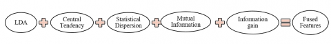
In this research work, the features like Linear Discriminant Analysis (LDA), central tendency (Weighted arithmetic mean, Winsorized mean, standard deviation), Statistical dispersion (Interquartile range (IQR), Median Absolute Deviation (MAD)), Mutual Information and Information Gain, are extracted. Figure 7 shows the Feature Extraction phase. The feature extraction phase is shown diagrammatically in Figure 5.
Figure 7. Feature extraction
4.2.1 LDA
A popular dimensionality reduction method for supervised classification issues is LDA. The objective of LDA is to maximise class separability while projecting the dataset onto a lower-dimensional space, wherever the highest division of the distinct types is found within all feasible one-dimension group. In such a scenario, the actual computation of LDA mapping coefficients is predicated on maximisation of functional built through supplied data related to the actual classes. Construction of a functional optimization: Using two datasets $Y_1$ and $Y_2$ in d-dimensional feature space, with mass centers (averages) $a_1$ and $a_2$, detect the vector of LDA mapping factors $n^* \in \mathbb{R}^b$ which would increase functional $A: \mathbb{R}^b \rightarrow \mathbb{R}$. Considering Formula is performed in Eq. (21)-(23).
$n^*=\underset{n}{\operatorname{argmax}} c(a), A(n)=\frac{n^{T T} d_e n}{n^{T T} n_n n}$ (21)
While,
$d_e=\left(a_1-a_2\right)\left(a_1-a_2\right)^{T T}$ (22)
$d_n=\sum_{g \in 1}, \sum_{f \in y_g}\left(f-a_g\right)$ (23)
4.2.2 Central tendency
Central tendency relates to a central or typical evaluate in a file that represents the entire set of values. It is a statistical measure that summarizes the central location of a set of values.
Weighted arithmetic mean: The weighted arithmetic mean is a type of mean in which different values in a data set are given different weights to reflect their relative importance. It is intended by expanding each value by its mass, summing the product, and partitioning by the sum of the weights. The weighted mean is often used when the values in a data set represent different quantities, such as - in cases, where the values represent the number of items sold or the amount of money earned. By assigning weights to the values, the weighted mean considers the relative importance of each value in the computation, providing a more accurate representation of the central tendency of the data. The formula for Weighted Arithmetic Mean is mathematically shown in Eq. (24).
$\bar{h}_i=\frac{i_1 h_1+i_2 h_2+i_3 h_3+\cdots \ldots+i_k h_k}{i_1+i_2+i_3+\cdots \ldots \ldots+i_k}=\frac{\sum_{j=1}^k i_j h_j}{\sum_{j=1}^k i_j}$ (24)
Here, $i_1$ is the weight for non-negative data that is not negative. $h_j, j=1,2, \ldots, k$. The weights assigned to the set of observations are used to calculate the weighted arithmetic mean, which is an average. In this case, the Weighted Arithmetic Mean is simply the arithmetic mean. Systems of data analysis, weighted differential, and integral calculus all heavily depend on the weighted arithmetic mean.
Winsorized mean Winsorized mean is a reliable statistical measure that lessens the effect of outliers on the average. Extreme values, typically the highest and lowest percentiles, are replaced with less extreme values falling within a given range. An estimate of a dataset's central tendency that is more reliable and representative is provided by the resulting Winsorized mean. A symmetric probability distribution's mean can be estimated using the winsorized mean, which is a reliable estimator. It is also discovered to be more effective than a few other robust estimators, including the trimmed mean. Winsorizing follows the same steps as trimmed means, but the extreme value(s) are replaced with the less extreme adjacent values rather than being dropped.
SD: The SD is a helpful spread measurement for equal variances. In normal distributions, info is proportionately distributed and deviation. Values decrease as one moves away from the centre, where they tend to concentrate in a relatively small area. By examining the standard deviation, you can determine how far your data are, on average, from the centre of the distribution. Among the research possibilities with normal distributions are height, scores on standardised tests, and job satisfaction scores. To make suppositions about the higher populations they were taken, statistical tests can be used to compare the standard deviations of various samples. SD is mathematically shown in Eq. (25).
$\sigma=\sqrt{\frac{\sum(Z-\mu)^2}{N v}}$ (25)
where, $\sigma$ is the Population SD, $Z$ represent all value, $\mu$ is the population Mean, $N v$ is the number of rates in population.
4.2.3 Statistical dispersion
A measure of a set of values' statistical dispersion is known as statistical dispersion. It shows how far away from the data set's central tendency values in a data set are. Measures of dispersion provide important information about the distribution of principles in a data set and can be used to determine outliers and skewness. They can also be used to make comparisons between data sets and to quantify the uncertainty or risk associated with predictions based on the data.
IQR: IQR is a appraise of the dispersion of a continuous data set, delimited as the distinction with both the 75th and 25th percentiles, and the upper and lower quartiles. It is used as a robust summary statistic, as it is not sensitive to outliers or uttermost values in data. The IQR is a useful tool for identifying and removing outliers, as values outside of the range of 1.5 times the IQR from the topmost and lower quartiles are often considered to be outliers. IQR is mathematically shown in Eq. (26):
$I Q R=Q 3-Q 1$ (26)
where, Q1 is less quartile and Q3 is superior quartile. The IQR represents the range of values that encompasses the core 50% of the file, and is a measure of the spread of the data.
MAD: When the deviation value needs to be less impacted by extreme values in the tail, the median absolute deviation is used instead of the mean deviation. The median is less impacted by the tail values than the mean, which accounts for this. The mathematical model is shown in Eq. (27).
$M A D=\operatorname{median}\left(X X_i-m d\right)$ (27)
$X X_i$ is the contested dataset, $m d$ is the median of a dataset.
4.2.4 Mutual information
Two continuous random variables are $A$ and $B$ with joint Probability Density Function (PDF) $(m, o)$, $l(m)$ and $l(o)$ are small pdfs. MI in $A$ and $B$ is specified in Eq. (28).
$I(A ; B)=\iint l(m, o) \log \frac{l(m, o)}{l(m) l(o)}$ pmpo (28)
Review tri discrete random variables $A$ and $B$, with scripts $\alpha$ and $\beta$, individually. The MI enclosed by $A$ and $B$ with a joint probability mass function $l(m, o)$ also marginal probabilities $l(m)$ and $l(o)$ is defined in Eq. (29).
$I(A ; B)=\sum_{m \in \alpha} \sum_{o \in \beta} l(m, o) \log \frac{l(m, o)}{l(m) l(o)}$ (29)
The MI differs from other dependency measures in two ways: first, it can measure any type of relationship between variables, and second, it is invariant to changes in spatial orientation.
4.2.5 Information gain
Information gain is a criterion used in information opinion to quantify the reduction in uncertainty or entropy of a random variable after observing some information. It is defined as the difference between the entropy of the system earlier and later, attentive for a particular attribute. Entropy formula is used to calculate Information gain, which measures the degree of disorder or randomness in a system. The information gain of an attribute is directly proportional to the reduction in the entropy of the target variable, and it is familiar with the chosen best attribute to data division at each access point in the tree.
5.1 Performance of individual deep learning models
The proposed methodology is implemented using PYTHON Google Colab. The suggested design has been analysed in connection to NMSE, MSRE, MSE, MAPE, RMSE.
i) NMSE
The operation of behavioural patterns is frequently appraised using the NMSE. It is typically measured in decibels and is defined in Eq. (30).
$N M S E=\frac{\sum_{x=1}^M \sum_{y=1}^N\left[d_{\text {in }}(p, q)-d_{\text {out }}(p, q)\right]^2}{\sum_{x=1}^M \sum_{y=1}^N\left[d_{\text {in }}(p, q)\right]^2}$ (30)
where, $M, N$ are the size of the matrix featuring a data, $d_{i n}(p, q)$ is a reference data, $d_{\text {out }}(p, q)$ is a tested data.
ii) MSRE
The average relative disparity between predicted values and actual estimates is measured by the MSRE. It is frequently employed in statistical analysis to assess the effectiveness of models. The mathematical model is shown in Eq. (31).
$M S R E=\frac{1}{n} \sum_1^n\left\{\frac{T_i-T_j}{T_j}\right\}^2$ (31)
where, $n$ is the amount of data points, $T_i$ is the actual data and $T_j$ is the predicted data.
iii) MSE
The amount of error in statistical models is gauged by the Mean Squared Error, or MSE. Amongst the noticed and predicted principles, it measures the average squared difference. The MSE is equivalent to zero when a model is faultless. The price growths as model error performs equally. Mathematical model is shown in Eq. (32).
$M S E=\frac{1}{n} \sum_{r=1}^n\left(T_i-T_j\right)^2$ (32)
where, $n$ is the amount of data points, $T_i$ is the actual data and $T_j$ is the predicted data.
iv) MAPE
A model's ability to predict or forecast a variable accurately is measured by MAPE. In a dataset, it determines the typical percentage dissimilarity between some values. The arithmetical model is shown in Eq. (33).
$M A P E=\frac{100 \%}{n} \sum_{r=1}^n\left|\frac{K_r-H_r}{K_r}\right|$ (33)
where, $H_r$ is the amount of false classifications, $K_r$ is the total of real classifications.
v) RMSE
Among the techniques most often exploited to measure the correctness of predictions is RMSE. It demonstrates the Euclidean distance separating predictions and Realistic quantification. The mathematical model is shown in Eq. (34).
$R M S E=\sqrt{\frac{1}{n} \sum_{r=1}^n\left(K_r-H_r\right)}$ (34)
where, $H_r$ is the several of false classifications, $K_r$ is the count of true classifications.
5.2 Ensemble model performance analysis
The Table 6 shows the performance metrics of six different models - AGTO, TLO, RNN, LSTM, KNN, and Proposed - evaluated using five different metrics: MSE, MSRE, NMSE, RMSE, and MAPE. Located on the provided results, the Proposed model appears to have the best overall presentation, as it has the lowest scores for MSE, MSRE, and RMSE, and the second-lowest scores for NMSE and MAPE. This suggests that the Proposed model has the lowest average squared difference, lowest average percentage difference, and lowest root mean squared distinction amongst the expected values and actual values. In contrast, RNN has the highest MSRE score, indicating that it has the largest relative error amid the predicted and factual values. The KNN model has the highest NMSE score, indicating that it has the largest normalized error among the six models. However, it is excellent noting that the variations in the scores among the six models are relatively small.
The Table 7 represents the performance evaluation of different models, AGTO, TLO, RNN, LSTM, KNN, and a proposed model based on five different metrics: MSE, MSRE, NMSE, RMSE, and MAPE. From the table, the suggested template outperformed all the diverse models on all the rating metrics, except for MAPE, where it is slightly worse than the KNN model. In terms of MSE, MSRE, NMSE, and RMSE, the proposed model achieved the lowest values, indicating its superior performance in predicting the target variable compared to the other models. The diminish in the values of these metrics, the finer the model's presentation in terms of accuracy and precision. In contrast, for MAPE, the proposed model's performance is slightly worse than the KNN model. However, MAPE is a percentage-based metric, and its interpretation varies depending on the scale of the target variable.
From the Table 8 analysis, while comparing the existing methods with proposed, it has obtained low values.
Table 9 and Table 10 show the MSE, MSRE, NMSE, RMSE and MAPE values of Without Pre-processing, With PRE-PROCESSING, Without Feature Extraction and With Feature Selection.
The MSE comparison of the proposed and existing methods AGTO, TLO, RNN, LSTM, KNN is shown in the Figure 8. The MSE for the suggested approach is decreased when compared with existing approaches. The proposed has 0.312638 MSE in Plant 1 metrics, 0.252873 MSE in Plant 2 metrics.
Table 6. Metrices-Plant1
|
|
AGTO |
TLO |
RNN |
LSTM |
KNN |
Proposed |
|
MSE |
0.327284 |
0.343531 |
0.34068 |
0.325228 |
0.353628 |
0.312638 |
|
MSRE |
0.3034 |
0.335287 |
0.294314 |
0.349261 |
0.315746 |
0.290741 |
|
NMSE |
0.441479 |
0.475173 |
0.444496 |
0.472143 |
0.468562 |
0.422365 |
|
RMSE |
0.408064 |
0.38661 |
0.355911 |
0.409722 |
0.379244 |
0.372732 |
|
MAPE |
0.320739 |
0.33666 |
0.333866 |
0.318724 |
0.346556 |
0.306385 |
Table 7. Metrices-Plant2
|
|
AGTO |
TLO |
RNN |
LSTM |
KNN |
Proposed |
|
MSE |
0.27786 |
0.286027 |
0.263056 |
0.264719 |
0.275554 |
0.252873 |
|
MSRE |
0.271192 |
0.255387 |
0.282495 |
0.245401 |
0.238052 |
0.235162 |
|
NMSE |
0.415083 |
0.409309 |
0.412437 |
0.385651 |
0.388286 |
0.368954 |
|
RMSE |
0.245809 |
0.231482 |
0.256053 |
0.222432 |
0.21577 |
0.21315 |
|
MAPE |
0.276636 |
0.285177 |
0.328283 |
0.296781 |
0.315148 |
0.273277 |
Table 8. Metrices - Analysis1
|
|
DBN+GC+TLBO |
DCNN+GC+TLBO |
RNN+GC+TLBO |
Proposed |
|
MSE |
0.347897 |
0.329361 |
0.331444 |
0.312638 |
|
MSRE |
0.339548 |
0.3537 |
0.307256 |
0.290741 |
|
NMSE |
0.481211 |
0.478143 |
0.44709 |
0.422365 |
|
RMSE |
0.391523 |
0.414928 |
0.41325 |
0.372732 |
|
MAPE |
0.340939 |
0.322774 |
0.324815 |
0.306385 |
Table 9. Metrices - Analysis2
|
|
Without Pre-Processing |
With Pre-Processing |
|
MSE |
0.345009 |
0.312638 |
|
MSRE |
0.298054 |
0.290741 |
|
NMSE |
0.450144 |
0.422365 |
|
RMSE |
0.360434 |
0.372732 |
|
MAPE |
0.338109 |
0.306385 |
Table 10. Metrices - Analysis3
|
|
Without Feature Selection |
With Feature Selection |
|
MSE |
0.358122 |
0.312638 |
|
MSRE |
0.319759 |
0.290741 |
|
NMSE |
0.474517 |
0.422365 |
|
RMSE |
0.384063 |
0.372732 |
|
MAPE |
0.35096 |
0.306385 |
Figure 9 displays the MSRE comparison of the proposed and existing methods AGTO, TLO, RNN, LSTM, and KNN. When compared to current approaches, the suggested approach's MSRE is lower. The proposed has metrics for 0.235162 MSRE in Plant 2 and 0.290741 MSRE in Plant 1.
Figure 10 depicts the NMSE comparison of the proposed and existing methods AGTO, TLO, RNN, LSTM, and KNN. When compared to current approaches, the suggested approach's NMSE is lower. The proposed has NMSE values of 0.368954 for Plant 2 metrics and 0.422365 for Plant 1 metrics.
The RMSE comparison of the proposed and existing methods AGTO, TLO, RNN, LSTM, KNN is shown in the above Figure 11. The RMSE for the suggested approach is reduced when compared with existing approaches. The proposed has 0.372732RMSE in Plant 1 metrics, 0.21315RMSE in Plant 2 metrics.
The MAPE comparison of the proposed and existing methods AGTO, TLO, RNN, LSTM, KNN is shown in the above Figure 12. The MAPE for the suggested approach is reduced when compared with existing approaches. The proposed has 0.306385 MAPE in Plant 1 metrics, 0.273277 NMSE in Plant 2 metrics.
Figure 8. Performance of MSE
Figure 9. Performance of MSRE
Figure 10. Performance of NMSE
Figure 11. Performance of RMSE
Figure 12. Performance of MAPE
5.3 Insights and implications for solar power integration
The development of intelligent control systems that can manage the fusion of various renewable energy sources, including solar power, represents a promising area of research. This would entail creating algorithms and models that can forecast the output of various renewable energy sources based on the weather and other variables, and then optimally allocating resources to make sure that the grid receives a steady and dependable supply of energy. Such systems might also include methods for demand-side management to assist in real-time balancing of energy supply and demand. Intelligent control systems could significantly reduce the reliance on non-renewable energy sources by optimising the integration of numerous renewable energy sources, thereby promoting a more sustainable and dependable energy future.
The GC-TLBO Algorithm was a proposed hybrid optimisation approach that conceptually combines the standard Artificial GTO and TLBO. Using the new ensembled deep learning model, which combines the O-RNN, DBN, and DCNN, solar power forecasting was carried out. The O-RNN, which receives the outcomes from DBN and DCNN. With the help of the chosen ideal features obtained using GC-TLBO, the DBN and DCNN are trained. Utilising GC-TLBO, the RNN's weight is adjusted. Overall, the conclusions suggest that the proposed model, which incorporates a hybrid optimization approach and an ensembled DL model, is a promising technique for accurately forecasting solar power generation. Based on the plant 2 results, the proposed outperformed the other models in terms of MSE, MSRE, and RMSE, with values of 0.252873, 0.235162, and 0.21315, respectively. The LSTM model also performed well, with low values of MSE, MSRE, and RMSE. In terms of NMSE, all models performed similarly, with values ranging from 0.368954 to 0.415083. This indicates that the models had similar levels of accuracy in predicting the data. The MAPE values varied among the models, with the proposed model having the lowest value of 0.273277. This indicates that the proposed model had the lowest average percentage error in predicting the data. Overall, the proposed model showed promising results and outperformed the other models in several metrics. The training and fine-tuning of the models can require a significant amount of computing power and time, which may not be feasible for all applications. The accuracy of the model may be affected by factors such as missing or inaccurate data, as well as the choice of feature extraction and selection techniques. For the future, weather parameters could be used as input range, nature-inspired algorithms could be used to train neurons, and exceed hybrid techniques could be used to enhance neural network performance in the context of quicker and more accurate forecasting.
[1] Bacher, P., Madsen, H., Nielsen, H.A. (2009). Online short-term solar power forecasting. Solar Energy, 83(10): 1772-1783. https://doi.org/10.1016/j.solener.2009.05.016
[2] Wan, C., Zhao, J., Song, Y., Xu, Z., Lin, J., Hu, Z. (2015). Photovoltaic and solar power forecasting for smart grid energy management. CSEE Journal of Power and Energy Systems, 1(4): 38-46. https://doi.org/10.17775/CSEEJPES.2015.00046
[3] Ren, Y., Suganthan, P.N., Srikanth, N. (2015). Ensemble methods for wind and solar power forecasting—A state-of-the-art review. Renewable and Sustainable Energy Reviews, 50: 82-91. https://doi.org/10.1016/j.rser.2015.04.081
[4] Wang, H., Liu, Y., Zhou, B., Li, C., Cao, G., Voropai, N., Barakhtenko, E. (2020). Taxonomy research of artificial intelligence for deterministic solar power forecasting. Energy Conversion and Management, 214: 112909. https://doi.org/10.1016/j.enconman.2020.112909
[5] Martinez-Anido, C.B., Botor, B., Florita, A.R., Draxl, C., Lu, S., Hamann, H.F., Hodge, B.M. (2016). The value of day-ahead solar power forecasting improvement. Solar Energy, 129: 192-203. https://doi.org/10.1016/j.solener.2016.01.049
[6] Bessa, R.J., Trindade, A., Miranda, V. (2014). Spatial-temporal solar power forecasting for smart grids. IEEE Transactions on Industrial Informatics, 11(1): 232-241. https://doi.org/10.1109/TII.2014.2365703
[7] Zhang, J., Florita, A., Hodge, B.M., Lu, S., Hamann, H.F., Banunarayanan, V., Brockway, A.M. (2015). A suite of metrics for assessing the performance of solar power forecasting. Solar Energy, 111: 157-175. https://doi.org/10.1016/j.solener.2014.10.016
[8] Zhang, X., Li, Y., Lu, S., Hamann, H.F., Hodge, B.M., Lehman, B. (2018). A solar time based analog ensemble method for regional solar power forecasting. IEEE Transactions on Sustainable Energy, 10(1): 268-279. https://doi.org/10.1109/TSTE.2018.2832634
[9] Wang, J., Zhong, H., Lai, X., Xia, Q., Wang, Y., Kang, C. (2017). Exploring key weather factors from analytical modeling toward improved solar power forecasting. IEEE Transactions on Smart Grid, 10(2): 1417-1427. https://doi.org/10.1109/TSG.2017.2766022
[10] Persson, C., Bacher, P., Shiga, T., Madsen, H. (2017). Multi-site solar power forecasting using gradient boosted regression trees. Solar Energy, 150: 423-436. https://doi.org/10.1016/j.solener.2017.04.066
[11] He, Y., Wang, Y. (2021). Short-term wind power prediction based on EEMD–LASSO–QRNN model. Applied Soft Computing, 105: 107288. https://doi.org/10.1016/j.asoc.2021.107288
[12] Bozorg, M., Bracale, A., Carpita, M., De Falco, P., Mottola, F., Proto, D. (2021). Bayesian bootstrapping in real-time probabilistic photovoltaic power forecasting. Solar Energy, 225: 577-590. https://doi.org/10.1016/j.solener.2021.07.063
[13] Das, U.K., Tey, K.S., Idris, M.Y.I.B., Mekhilef, S., Seyedmahmoudian, M., Stojcevski, A., Horan, B. (2022). Optimized support vector regression-based model for solar power generation forecasting on the basis of online weather reports. IEEE Access, 10: 15594-15604. https://doi.org/10.1109/ACCESS.2022.3148821
[14] Liu, C.H., Gu, J.C., Yang, M.T. (2021). A simplified LSTM neural networks for one day-ahead solar power forecasting. IEEE Access, 9: 17174-17195. https://doi.org/10.1109/ACCESS.2021.3053638
[15] Wu, Z., Wang, B. (2021). An ensemble neural network based on variational mode decomposition and an improved sparrow search algorithm for wind and solar power forecasting. IEEE Access, 9: 166709-166719. https://doi.org/10.1109/ACCESS.2021.3136387
[16] Yang, Z., Mourshed, M., Liu, K., Xu, X., Feng, S. (2020). A novel competitive swarm optimized RBF neural network model for short-term solar power generation forecasting. Neurocomputing, 397, 415-421. https://doi.org/10.1016/j.neucom.2019.09.110
[17] Bendali, W., Saber, I., Bourachdi, B., Amri, O., Boussetta, M., Mourad, Y. (2022). Multi time horizon ahead solar irradiation prediction using GRU, PCA, and GRID SEARCH based on multivariate datasets. Journal Européen des Systèmes Automatisés, 55(1): 11-23. https://doi.org/10.18280/jesa.550102
[18] Lee, W., Kim, K., Park, J., Kim, J., Kim, Y. (2018). Forecasting solar power using long-short term memory and convolutional neural networks. IEEE Access, 6: 73068-73080. https://doi.org/10.1109/ACCESS.2018.2883330
[19] Singla, A., Singh, K., Yadav, V.K. (2020). Optimization of distributed solar photovoltaic power generation in day-ahead electricity market incorporating irradiance uncertainty. Journal of Modern Power Systems and Clean Energy, 9(3): 545-560. https://doi.org/10.35833/MPCE.2019.000164
[20] Suksamosorn, S., Hoonchareon, N., Songsiri, J. (2021). Post-processing of NWP forecasts using Kalman filtering with operational constraints for day-ahead solar power forecasting in Thailand. IEEE Access, 9: 105409-105423. https://doi.org/10.1109/ACCESS.2021.3099481
[21] Das, U.K., Tey, K.S., Idris, M.Y.I.B., Mekhilef, S., Seyedmahmoudian, M., Stojcevski, A., Horan, B. (2022). Optimized support vector regression-based model for solar power generation forecasting on the basis of online weather reports. IEEE Access, 10: 15594-15604. https://doi.org/10.1109/ACCESS.2022.3148821
[22] Aslam, M., Lee, S.J., Khang, S.H., Hong, S. (2021). Two-stage attention over LSTM with Bayesian optimization for day-ahead solar power forecasting. IEEE Access, 9: 107387-107398. https://doi.org/10.1109/ACCESS.2021.3100105
[23] Elsaraiti, M., Merabet, A. (2022). Solar power forecasting using deep learning techniques. IEEE Access, 10: 31692-31698. https://doi.org/10.1109/ACCESS.2022.3160484
[24] Moayedi, H., Mosavi, A. (2021). An innovative metaheuristic strategy for solar energy management through a neural networks framework. Energies, 14(4): 1196. https://doi.org/10.3390/en14041196
[25] Ghadimi, N., Akbarimajd, A., Shayeghi, H., Abedinia, O. (2018). Two stage forecast engine with feature selection technique and improved meta-heuristic algorithm for electricity load forecasting. Energy, 161: 130-142. https://doi.org/10.1016/j.energy.2018.07.088
[26] Pan, C., Tan, J. (2019). Day-ahead hourly forecasting of solar generation based on cluster analysis and ensemble model. IEEE Access, 7: 112921-112930. https://doi.org/10.1109/ACCESS.2019.2935273
[27] Sheng, H., Ray, B., Chen, K., Cheng, Y. (2020). Solar power forecasting based on domain adaptive learning. IEEE Access, 8: 198580-198590. https://doi.org/10.1109/ACCESS.2020.3034100