Sara Ali Abd Al Hussen*![]() | Elham Mohammed Thabit A. Alsaadi
| Elham Mohammed Thabit A. Alsaadi![]()
© 2023 IIETA. This article is published by IIETA and is licensed under the CC BY 4.0 license (http://creativecommons.org/licenses/by/4.0/).
OPEN ACCESS
The need for automated diagnostic systems in medical imaging, particularly in the detection and categorization of brain tumors, is paramount. This research proposes a hybrid model to identify and classify MRI-detected brain tumors into four categories: pituitary, meningioma, glioma, or absence of a tumor. This hybrid approach leverages the strengths of both deep learning and traditional machine learning techniques, enabling the extraction of complex features and the recognition of intricate patterns, such as those found in brain tumors. Machine learning further enhances the model's capacity to classify accurately based on these specific features, reducing time and cost. The proposed system consists of several stages: initial pre-processing of brain MRI images, the application of two distinct segmentation techniques (region-based and edge-based), morphological operations, feature extraction, and finally classification. The classification employs a hybrid model (VGG16) in conjunction with four traditional classifiers: Support Vector Machine (SVM), Naive Bayes (NB), Decision Tree (DT), and Random Forest (RF). The experimental results highlight that the use of Random Forest with region-based segmentation yields the highest accuracy, reaching 99.17%. This combination excels at focusing on minute yet crucial details in MRI images and maintains stability in the presence of distortion and outliers. The dataset employed in this study is an amalgamation of three: Figshare, SARTAJ, and Br35H, each containing MRI images of the aforementioned four types of brain tumors.
brain tumor, machine learning, magnetic resonance imaging (MRI), segmentation, classification, VGG16
The brain, acting as the epicenter of the body's central nervous system, is tasked with orchestrating a myriad of actions via thousands of neurons and countless connections [1]. The emergence of computer-aided diagnostic tools (CAD), such as those utilized in Android games, has revolutionized the early detection of brain tumors [2]. Brain tumors are characterized by unregulated and abnormal cell proliferation within the brain, leading to fatal outcomes if not promptly detected. The malignant nature of certain tumors necessitates their early detection to prevent widespread invasion within the brain [3].
Brain tumors can be classified into primary and secondary types. The former originates within the brain, while the latter, although detected in the brain, stems from other regions of the body [4]. The impetus behind this research is the labor-intensive and skill-dependent process of tumor diagnosis via medical imaging. Experts like radiologists meticulously examine images from CT scans, MRI scans, and positron emission tomography scans, forming the basis for subsequent treatment recommendations. This taxing process often spans several hours, underscoring the need for automation to expedite the detection process [5].
Significant research efforts have been channeled into segmentation in medical imaging, including cancer detection in the brain, lungs and breasts [6].
The complexity of brain tumor detection lies in the variability of tumor tissue properties, locations, shapes, sizes, and intensities across different patients, coupled with often unclear and irregular tumor boundaries [7]. This necessitates the development of advanced techniques anchored in deep learning and machine learning. CAD systems, encompassing deep learning and machine learning-based diagnostic systems, are founded on principles of magnetic resonance imaging (MRI), a cornerstone modality in medical imaging [8, 9]. MRI is routinely employed to visualize aberrant brain tissues [10]. Given its capacity to deliver high-resolution brain data, MRI facilitates swift diagnosis of brain anomalies [11]. The efficacy of the final detection system hinges on the reliability and robustness of each stage [12].
In this study, a hybrid model (VGG16) combined with four conventional classifiers (SVM, NB, DT, and RF) is utilized to categorize four distinct types of brain tumors. The remainder of the paper is organized as follows: Section 2 delineates the related works. The proposed approach for brain tumor detection is elaborated in Section 3. Segmentation is discussed in Section 4, while feature extraction is expounded in Section 5. Classification is covered in Section 6, and the Evaluation Metrics findings are presented in Section 7. The results and discussion are provided in Section 8, culminating in the conclusion in Section 9.
Our work is committed to the development of a brain tumor detection model that employs two segmentation methods, namely region-based segmentation and edge-based segmentation. A hybrid system, VGG16, in conjunction with four conventional classifiers (SVM, DT, RF, and NB), is utilized to categorize MRI images of four distinct types of human brain tumors. In this section, related works in the field are explored.
A technique formulated by Minz and Mahobiya [13] utilized the AdaBoost algorithm for machine learning, aiming at the automatic classification of anticipated brain images. The proposed system was partitioned into three distinct components: pre-processing, grayscale image conversion, and threshold segmentation and averaging filtering.
Abbasi and Tajeripour [14] proposed a method that incorporated data pre-processing through bias field correction and graph matching. The classification of data was executed using random forest, resulting in exceptional classification accuracy.
Malathi and Sinthia [15] employed convolutional neural network (CNN) technology for brain tumor segmentation. They applied the TensorFlow package to execute complex mathematical operations on high-quality glioma data, obtained from the BRATS 2015 dataset.
Arunkumar et al. [16] suggested an automated technique for segmenting and detecting brain tumors using artificial neural networks (ANN). The model achieved an accuracy of 94.07%, a sensitivity of 90.09%, and a specificity of 96.78%.
Pravitasari et al. [17] proposed a novel ROI and ROI classification architecture combined with the UNet-VGG16 fully convolutional network. The model achieved an impressive 96.1% accuracy on the learning dataset.
Sameer et al. [18] introduced an idea for improving image contrast in MRI images using adaptive histogram equalization (AHE). The U-NET algorithm was used in their research to create a fully automated hashing system, which achieved 96% and 98.5% accuracy rates using 5-fold and 10-fold, respectively.
Basha et al. [19] utilized a variety of neural network technologies and a several-step process that included system training, pre-processing, and application to brain MRI images. Their model reported an accuracy of 94%.
Sharif et al. [20] deployed the Inception-v3 architecture, based on CNN, to segment brain tumors. The project's progress was assessed using the BRATS 2013, BRATS 2014, BRATS 2017, and BRATS 2018 datasets, resulting in an average accuracy rate of 92%.
Raja [21] developed a classification for brain malignancies using a hybrid deep auto-encoder and a segmentation technique based on Bayesian fuzzy clustering.
Kumar et al. [22] proposed an automated system for classifying brain cancers in MRI images using K-nearest neighbor. Their method achieved an accuracy of 96.5%, a sensitivity of 100%, and a specificity of 93%.
Habib et al. [23] suggested a process, which included noise reduction, image enhancement as part of the pre-processing stage, and image segmentation using multiple algorithms. The study reported an SVM classifier accuracy of 90% after segmentation of the texture and shape-based features.
These studies collectively underscore the strides made in the field, setting the stage for our research in enhancing brain tumor detection efficiency.
Lastly, A technique formulated by Chellakh et al. [24] employed the DRB classifier to perform the MRI brain tumor classification tasks. The deep features were extracted by deep learning models such as AlexNet, ResNet50, ResNet-18, and VGG-16. An accuracy of 79.19% was obtained with AlexNet, 81.73% with VGG-16, 78.17% with ResNet50, and 80.46% with ResNet18 surpassing SVM, KNN and decision tree techniques.
These studies collectively underscore the strides made in the field, setting the stage for our research in enhancing brain tumor detection efficiency.
The proposed method uses a hybrid model (VGG16) with four conventional classifiers supporting vector machine (SVM), decision tree (DT), random forest (RF), and Nine Bayes (NB) to automate the detection and prognosis of human brain cancers. The main objective of this research is to develop a high-performance, accurate and simple automated system for brain tumor classification.
3.1 Methodology
The proposed system consists of several steps:
Step1: The input dataset MRI with gray scale channels and splitting data into train and test.
Step2: pre-processing.
Step3: Segmentation is done using region-based segmentation, and edge-based segmentation.
Step4: Feature extraction is done using pre-trained VGG16.
Step5: Build classifiers (machine learning algorithm).
Step6: Classification by traditional classifires.
Accuracy, precision, recall, and F1-score were used to gauge the model's effectiveness. Depending on the requirements of the task and the nature of the problem, use these measurements. It is important to choose metrics commensurate with the desired objective and balance considerations between accuracy and detection.
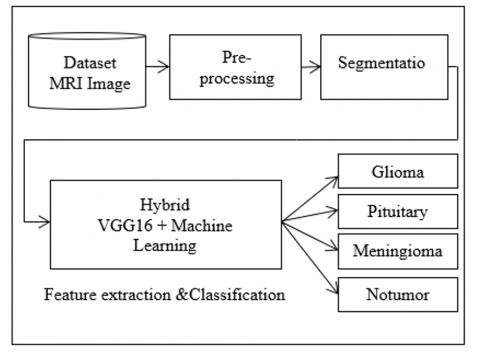
Figure 1 depicts the proposed scheme's schematic. The specifics for each action are as follows:
Figure 1. Diagram of the proposed scheme
3.2 Dataset description
The dataset used to implement the proposed system is the brain tumor MRI dataset. This dataset has been chosen due to it is intended to detect different types of brain tumors. The dataset combines information from the Fig share, SARTAJ, and Br35H dataset [25]. This dataset contains 7022 MRI images of the human brain that were classified into four categories: Glioma meningioma - no tumor and pituitary. No tumor class images were taken from the Br35H dataset. The SARTAJ dataset had a problem: the glioma category images were not labeled correctly, so images on Fig share were used instead. The dataset was obtained from the website: (https://www.kaggle.com/datasets/masoudnickparvar/brain-tumor-mri-dataset. Figure 2 represents samples from the data set. Data split the percentages of training, and testing data are determined, with 80 % of training data, and 20% testing data are. This is the ratio given the best result. Table 1 shows distribution of the dataset into training and test images.
Figure 2. A sample image of MRI dataset
Table 1. Distribution of the dataset into training and test images
|
Type |
Glioma |
Meningioma |
Pituitary |
Normal |
|
Total |
1621 |
1645 |
1757 |
2000 |
|
Train |
1321 |
1339 |
1457 |
1595 |
|
Test |
300 |
306 |
300 |
405 |
3.3 Pre-processing
This step involves removing noise from images and improving their quality. Smoothing and contrast enhancement techniques are employed to enhance details and make tumors more noticeable. To get greater outcomes, you must always have better image quality. Pre-processing greatly facilitates the transmission of the image's enhanced characteristics. The primary objective of this stage is to enhance the image's symmetry or visual appeal. It is common practice to utilize data pre-processing to lower image contrast, undesirable noise, and brightness. Pre-Processing includes the following procedures:
3.3.1 Resize
The dataset consists of thousands of images of varying sizes, as mentioned in Subsection 2.1. In order to standardize image sizes, we use pre-processing. All of the images in the collection are resized to 200 × 200 pixels. Changing and reducing the size of the images to 200 × 200 is necessary because it facilitates their processing and analysis and reduces the training and testing time of the models, which contributes to improving efficiency of the process.
3.3.2 Normalization
Normalization helps improve the training and stability of the models. Normalizing images also helps avoid the effect of color contrast and brightness on model performance. It is essential in image pre-processing, each pixel from the range [0-255] to [0-1] by utilizing the Eq. (1) min-max normalization rule.
$f(x-y)=\frac{f(x-y)-V\min }{V\max -V\min }$ (1)
3.3.3 Brightness
Refers to whether the image is overall light or dark.
3.3.4 Contrast
It is the variation in brightness between the image's items, and measures the amount of local differences present in the image. Image contrast can be calculated by the formula as shown in Eq. (2).
$cont=\sum\limits_{i=0}^{m-1}{\sum\limits_{j=0}^{n-1}{{{(x-y)}^{2}}}}f(x-y)$ (2)
3.3.5 Sharpness
Sharpness describes the clarity of detail in an image. Sharpening filters aim to draw attention to minute features. It reduces optical blur and sharpens edges. Sharpening filters are built on the concept of spatial distinction. It includes filters like the Difference, Laplacian, and Sobel.
A. Laplacian filters are derivative filters that are used to spot fast-changing edges in image.
B. Sobel filters are commonly used for edge detection.
C. In the direction that the selected mask points, differential filters enhance the details.
Image segmentation is the process of breaking an image down into smaller, more interpretable portions or discrete structural components. On the basis of some common edges, boundaries and features, these regions or units can be grouped. To find the position of the tumor in the MRI image, we used two segmentation methods: region-based segmentation and edge-based segmentation.
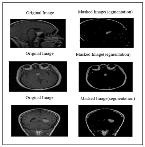
Figure 3. Sample region-based segmentation images
4.1 Segmentation for brain tumor using region-based segmentation
Region-based segmentation is a way to correctly identify and locate a desired area. Region split and merge segmentation is an image processing technique, we used in our work to segment an image. The split technique starts with the complete image based on a homogeneity criterion, such as grey levels, and if the homogeneity criterion is not met, repeatedly breaks each segment into quarters. Experiments and analyses depict that this method fast and accurate.
When the segmentation method is region-based segmentation, the best accuracy is obtained in the hybrid system: 99.17%.
Figure 3 displays an example region- based segmentation images.
4.2 Segmentation for brain tumor using edge- based segmentation
4.2.1 Canny-edge detection
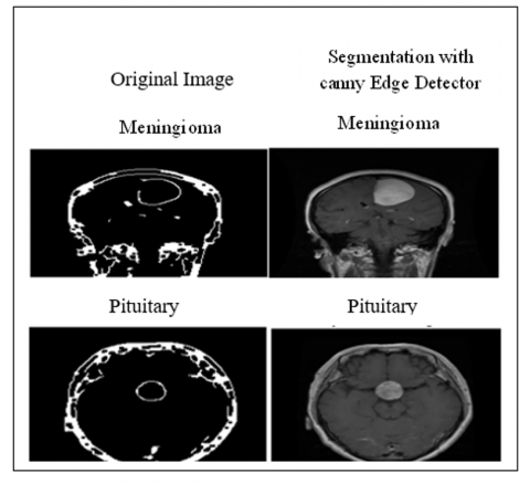
Undoubtedly one of the most well-known edge segmentation techniques is canny edge detection. It is based on the division of various visual components into groups. This algorithm's primary objective is to identify particular regions or portions of an image. The segmented sections are crucial for identifying certain picture components, such as malignancies. Additionally, it helps in locating the boundaries of the various areas of the image. By replacing their pixels with zeros, the undesired portions of the image can be quickly and readily removed. The dramatic intensity changes in the image are concentrated around the edges. The indicator of differences in an image's features is the intensity variation. Figure 4 displays an example segmented image.
Figure 4. Sample canny-edge segmentation images
When the segmentation method is edge-based segmentation, the best accuracy is obtained in the hybrid system: 89.84%. This percentage is lower compared to the hybrid system when using region-based segmentation.
4.3 Morphological operation
Morphological processes contribute to improving the quality of images and processing them to improve the performance of segmentation and analysis operations, improving the extraction of distinctive features from images, removing noise, rounding complex shapes, filling gaps, and repairing shapes, which leads to more accuracy results.
We used shutting operation in our work. To begin with, we filled in minor gaps and enlarged some areas of the MRI image using dilatation. Shapes with filling appear larger and lines appear thicker. The boundary region gains pixels as a result of the dilation procedure. We will obtain numerous interconnected regions in our photographs following dilatation. Second, we used erosion to eliminate pixels from object boundaries.
While erosion chooses the lowest value by comparing all pixel values near the input image, stretching chooses the largest value by comparing all pixel values in the area surrounding the input image that is describe by a structural element.
The following equations illustrate the morphological operations for tumor region detection. Eq. (3) illustrates the morphological function's dilation.
$I(dilate)S=\{I+S;for\text{ }all\text{ }pixels\text{ }in\text{ }I\in S\}$ (3)
The structural element utilized to determine the categorized image's pixel size can be seen here. Eq. (4) illustrates how the morphological function has eroded.
$I(eroded)S=\{I(eroded)S\}(eroded)S$ (4)
At this stage, part of the components is necessary, which is the process of converting data (image) into important elements, and advanced-level elements, such as shape, texture, color, and contrast, are collected. Once these features are present, each image is excluded from the numbers. that represent the extracted features. These representations may be in the form of two-dimensional vectors, where images are represented on pixels, or they may be converted to flat representations to describe features. Conversion of these features into the most important causes and contributes to providing appropriate data for models and types. This method is more smooth training and classification, wine stores data more efficiently, and facilitates calculations. This will be used to validate the model and its accuracy.
5.1 Transfer learning
In our proposed model, transfer learning was used in the field of machine learning, as it relies on the idea of using the experiences gained from one task to improve the performance of another task. The basic idea here is that models that have been pre-trained on a large and diverse data set (such as ImageNet) may be useful in extracting general features applicable to a specific task, such as classifying brain tumors.
The transfer learning strategy was chosen in this study because it saves time and effort, as training deep models from the beginning needs a lot of time and effort. By using pre-trained ImageNet models, part of this time and effort can be avoided. ImageNet pre-trained models are also trained on millions of images of different categories to extract useful features from the images. These pre-trained models contribute to model efficiency by taking advantage of weights and useful attributes that are pre-learned on ImageNet, reducing the need to train the model from scratch. This leads to an improvement in the performance of the model in classifying brain tumors.
5.1.1 VGG16
We used a pre-trained (CNN) construct (VGG16) available in the Keras library to extract features from images by passing them sequentially through multiple layers. These layers consist of convolutional layers that analyze features in images, pool layers that reduce dimensionality and remove unimportant details, and then reshape the extracted features into a one-dimensional vector suitable for feeding into a machine learning model.
Due to the small size of the image dataset and to avoid overfitting issues, we loaded the pre-trained VGG16 model onto the ImageNet dataset. The weights = 'imagenet' argument ensures that the model is initialized using the weights learned during training on the ImageNet dataset. The include_top = False argument means that the fully connected layers (top layers) of the VGG16 model will not be included, leaving only the convolutional base. Because brain tumors can be very different from the different objects displayed in ImageNet, there can be conflicts in the extracted features. For this reason, many layers are frozen in VGG16, in order to preserve features learned from ImageNet without affecting features learned from the tumor classification and detection task. Only the last fully connected layers are trained on the job of classifying brain tumors. The largest VGG16 architecture consists of 16 convolutional layers, three fully connected layers, and five pooling layers, with a maximum of 2 in each transformation layer, a linear SoftMax layer at the output, and a total of about 144 million parameters.
All fully linked layers use the ReLU activation function, which means that if the value generated by the input is greater than zero, the output is the same; If the value is less than or equal to zero, the result is zero. This function is easy to calculate and contributes to the activation of cell activation in neural networks. Fully connected layers also use dropout regularization to reduce overprocessing of training data and avoid overfitting.
VGG16 has the advantage of its ability to extract complex and overlapping features from images, and this improves model accuracy by providing an improved image representation that can identify similarities and differences between different tumors. For example, by extracting features related to shape, texture, color, and contrast, the model can recognize specific patterns such as tumor boundaries or subtle features within them.
When comparing the VGG16 architecture with other architectures such as ResNet or Inception. We find that VGG16 was chosen for this study for simplicity of its geometry based on repeated layers of small size, and this makes it easy to apply and achieve good results. It can also extract multiple and complex features from the images, which helps improve the model's performance in classifying tumors. The ability to freeze the first layers enhances the model's benefit from knowledge already gained from ImageNet without negatively affecting the performance of the tumor classification and detection task. Finally, it can handle a variety of images and discern complex patterns, which contributes to the generalization of the model to different tumors.
In the classification process, using a hybrid system (VGG16-Machine Learning).
With the help of the VGG16 model, features are taken out of the images. The images are converted into vectors through the model The next step is to feed the extracted features into one of the algorithms of the machine learning (SVM, NB, DT, RF) classifier to predict the classes as (glioma, pituitary, meningioma and no tumor). These models learn to classify tumors based on the extracted features.
In short, the hybrid system takes advantage of the advantages of each of the paradigms (neural networks and classical machine learning) to improve the classification and detection performance of brain tumors.
The main idea behind this system is to take advantage of each of the models' unique capabilities to improve the classification and detection performance of brain tumors.
The benefit of the hybrid system is to harness the power of neural networks as VGG16 has the ability to extract advanced features from images, which contributes to a complex and useful representation of tumors. Leveraging classic machine learning techniques such as SVM, DT, RF, and NB represent a different approach to classification and pattern learning, and can contribute to improved classification and detection performance.
Using a neural network model and classical machine learning techniques, multiple different representations of images can be taken advantage of, which contributes to an improved representation of tumors. Figure 5 displays hybrid system.
Figure 5. Hybrid VGG16-machine learning algorithms
The following traditional machine learning classifiers were used: (SVM), (NB), (DT), and (RF).
SVM is a powerful classifier used for classification tasks and is characterized by its ability to handle complex data sets and separate them into different classes. SVM overhauls the level of class separation by creating margins between data of different classes. SVM can handle complex classification problems and is able to handle nonlinear data using space transformations. It can be sensitive to the selection of training parameters and fine-tuning of the parameters that impair the classifier NB is a simple and powerful classifier used for classification which is based on Bayes assumptions for data analysis. NB works on class probabilities and features to make a rating decision. Works well for simple data and can be used for quick classification. It is based on specific assumptions regarding the independence between features which causes a weakening of the classifier.
DT divides data into classes through a set of sequential tests. It starts with a root and creates branches that represent tests and decisions, and is divided by the expected value of the class. Decisions can be easily understood and can be used for data with complex structures. It can lead to tree fusion, which causes a weakening of the classifier.
RF is a set of decision trees that work together to improve classification performance. It trains a set of decision trees on the same data and uses tree voting to make the final classification decision. It reduces the problem of tree joining and improves classification stability and accuracy. It may require additional training time and may be more complex than the individual algorithms and this causes weaknesses for the classifier.
The importance of classification plays an important part in understanding the objectives of the study and how to evaluate the performance of the model in classifying tumors. The categories focused on are:
(1) Glioma: This type of tumor refers to tumors that arise from the outer membranes of the brain. Classification of this type of tumor is important to determine the extent of the threat of the tumor and then take the necessary steps for treatment.
(2) Pituitary: This category refers to a tumor of the pituitary gland, Classification of this type of tumor can help determine its effects on hormones and bodily functions.
(3) Meningioma: These are tumors that arise from the nervous tissue in the meninges, which are parts of the central nervous system. Classification of this type of tumor can help determine the type of tumor and how much it affects nerves and vital functions.
(4) No tumor: This category means that there is no tumor in the submitted image. This category may be important to ensure the accuracy of negative classification and to ensure that no normal changes are converted into a misdiagnosis of tumors.
6.1 Classification challenges
Some classes may be more widespread than others, which leads to classification challenges due to the varying number of samples. This can lead to highlighting the most prevalent category and ignoring the less prevalent categories. Misclassification may occur when the model categorizes a sample into a category other than the correct one. This could be due to overlapping of traits between the classes or due to a lack of training data. It can be difficult to establish clear decision boundaries between some similar classes, thus complicating the task of classification.
The performance of the system for brain tumor detection and classification is evaluated in terms of effectiveness using the following metrics (accuracy, Precision, recall, F1 score and confusion matrix) because of its balance and its ability to provide a comprehensive view of tumor classification and detection. Eq. (5) remembering accuracy, Eq. (6) remembering accuracy, Eq. (7) remembering retrieval, and Eq. (8) remembering F1 score, confusion matrix for this model as shown in Table 2.
(1) Accuracy: the proportion of accurate (either positive or negative) findings to all available results. To acquire an overall notion of the model's categorization effectiveness, generic precision might be employed.
$Accuracy=\frac{TP+TN}{TP+TN+FP+FN}$ (5)
(2) Precision: measures the amount of correct positive outcomes (true positive and incorrect negative) divided by the sum of expected positive outcomes. Accuracy can be used to measure how accurately tumors are correctly classified as true tumors.
$Precision=\frac{TP}{TP+FP}$ (6)
(3) Recall: Measures the amount of true positive results (true positive and incorrect negative) divided by the sum of the actual positive results. Retrieval can be used to measure the ability of the model to detect all types of true tumors.
$Recall=\frac{TP}{TP+FN}$ (7)
(4) F1 Score: A balanced measure that combines accuracy and retrieval, balancing good detection with accurate classification. It can be useful for evaluating the overall performance of a model.
$F{{1}_{\text{Score }}}=\frac{2*(\text{ Recall })*(\text{ Precision })}{(\text{ Recall }+\text{ Precision })}$ (8)
(5) Confusion matrix: is an important tool for comprehensively evaluating classifiers, in which the relationships between correct and false classifications of the model. The confusion matrix consists of four main concepts: true positives (True Positives, TP), true negatives (True Negatives, TN), false positives (False Positives, FP), and false negatives (False Negatives, FN). The confusion matrix explains how the classifier deals with each category and how it begins with its classification in general. Table 2 explain the confusion matrix.
• True Positive (TP): The number of tumor images that have been classified correctly.
• True Negative (TN): The number of non-tumor images that are correctly classified.
• False Positive (FP): The number of non-neoplastic images that are misclassified as tumor.
• False negative (FN): The number of tumor images that are misclassified as non-tumor.
Diagonal elements (TP_X): These elements represent the correctly classified instances for each class. They show how well the classifier is doing in identifying each class correctly.
Off-diagonal elements (FN_X and FP_X): These elements show misclassifications.
7.1 Comparison of classifier performance
Metrics including accuracy, sensitivity, specificity, and general accuracy should be used to gauge classifier performance. In our investigation, it was discovered that RF performed better than the other classifiers due to the type of data it was trained on and the accuracy it achieved (99.17% compared to other classifiers).
We applied the hybrid model (VGG16 + machine learning classifiers (SVM, NB, DT, and RF)) using region-based segmentation and got the results classification report for this model as shown in below Tables 3-6.
Using an MRI image, the accuracy of each classifier is determined by deriving it from the confusion matrix.
The result is displayed in the following Figure 6, where the diagonal elements (297, 286, 399, and 293) reflect the correctly categorized photos for each category in the SVM confusion matrix.
The confusion matrix of DT's diagonal elements (312, 312, 386, and 246) represents the images that were correctly identified for each category. The outcome is depicted in Figure 7.
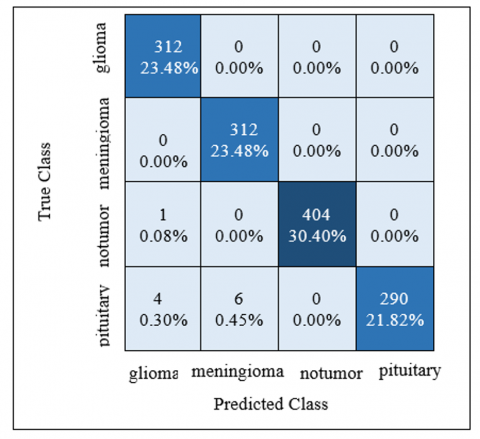
The confusion matrix of RF's diagonal elements (312, 312, 404, and 290) represent the images that were correctly identified for each category. The outcome is depicted in Figure 8.
The confusion matrix of NB's diagonal elements (308, 210, 363, and 231) represents the images that were correctly identified for each category. The outcome is depicted in Figure 9.
Table 2. Confusion matrix
|
|
|
True |
Class |
|
|
|
|
|
Glioma |
Meningioma |
No tumor |
Pituitary |
|
|
Glioma |
TP-G |
FN-G |
FN-G |
FN-G |
|
Predicted class |
Meningioma |
FP-M |
TP-M |
FN-M |
FN-M |
|
|
No tumor |
FP-N |
FN-N |
TP-N |
FN-N |
|
|
Pituitary |
FP-P |
FN-P |
FN-P |
TP-P |
Table 3. The performance evaluation of SVM
|
Classifiers |
Tumor Type |
Precision |
Recall |
F1-Score |
Support |
|
SVM |
Glioma |
0.95 |
0.95 |
0.95 |
312 |
|
|
Meningioma |
0.94 |
0.92 |
0.93 |
312 |
|
|
No tumor |
0.99 |
0.99 |
0.99 |
405 |
|
|
Pituitary |
0.95 |
0.98 |
0.96 |
300 |
Table 4. The performance evaluation of DT
|
Classifiers |
Tumor Type |
Precision |
Recall |
F1-Score |
Support |
|
DT |
Glioma |
0.93 |
1.00 |
0.96 |
312 |
|
|
Meningioma |
0.90 |
1.00 |
0.95 |
312 |
|
|
No tumor |
0.98 |
0.95 |
0.97 |
405 |
|
|
Pituitary |
0.97 |
0.82 |
0.89 |
300 |
Table 5. The performance evaluation of RF
|
Classifiers |
Tumor Type |
Precision |
Recall |
F1-Score |
Support |
|
RF |
Glioma |
0.98 |
1.00 |
0.99 |
312 |
|
|
Meningioma |
0.98 |
1.00 |
0.99 |
312 |
|
|
No tumor |
1.00 |
1.00 |
1.00 |
405 |
|
|
Pituitary |
1.00 |
0.97 |
0.98 |
300 |
Table 6. The performance evaluation of NB
|
Classifiers |
Tumor Type |
Precision |
Recall |
F1-Score |
Support |
|
NB |
Glioma |
0.77 |
0.99 |
0.86 |
312 |
|
|
Meningioma |
0.74 |
0.67 |
0.71 |
312 |
|
|
No tumor |
0.95 |
0.90 |
0.92 |
405 |
|
|
Pituitary |
0.88 |
0.77 |
0.82 |
300 |
Figure 6. The confusion matrix of SVM
Figure 7. The confusion matrix of DT
Figure 8. The confusion matrix of RF
Figure 9. The confusion matrix of NB
We ran several experiments on datasets available online. The reason for pick this dataset is that it aims to detect different types of brain tumors. The dataset involves 7,022 MRI scans of the human brain that were divided into four collections: pituitary, meningioma, glioma, and no tumor. Using MRI scans and segmentation technology, the precision from the confusion matrix is used to calculate the performance of each classifier. The two Tables 7 and 8 show the comparison of accuracy results between traditional machine learning classifiers using two segmentation methods, where the random forest with region-based segmentation achieved the best accuracy of 99.17%.
Table 7. Accuracy comparison among traditional machine learning classifiers by using Region–based segmentation
|
Segmentation Method |
Classifiers |
Accuracy |
|
Region–based segmentation |
SVM |
95.94 % |
|
|
DT |
94.51% |
|
|
RF |
99.17% |
|
|
NB |
83.67% |
In the region-based segmentation method, the selected region within the image represents the tumor-related information. This method was chosen because it focuses on the tumor region in particular, it can improve the model's capacity to discriminate between various tumor types. It contributes to focusing on regions that are important for classifying tumors, which can improve classification accuracy. On the negative side, important information outside the selected region may be ignored, which can affect the ability of the model to distinguish less obvious tumors.
Table 8. Accuracy comparison among traditional machine learning classifiers by using Edge–based segmentation
|
Segmentation Method |
Classifiers |
Accuracy |
|
Edge–based segmentation |
SVM |
93.75% |
|
|
DT |
91.35% |
|
|
RF |
98.87% |
|
|
NB |
81.64% |
In the edge-based segmentation method, the edges of shapes within the image are used to represent the different shapes and structures in tumors. They were chosen because the edges give important information about tumor structures and details that can contribute to their better characterization. It allows focusing on the fine structure of tumors and improves ability to distinguish the different details. On the negative side, it may increase the complexity and need more pre-processing.
For traditional classifiers such as (SVM, DT, RF, and NB) the segmentation methods may improve performance by providing distinct advantages for the classification.
Table 9. Comparison between our model proposed and related works
|
Author |
Methodology |
Accuracy |
|
Filatov and Yar [25] |
pretrained (CNN) ResNet50, EfficientNetB1, EfficientNetB7, EfficientNetV2B1. EfficientNetB1 showed the best results. |
87.67% |
|
Ullah et al. [26] |
combined of Gabor and ResNet50 and then classified by SVM |
95.73% |
|
Gómez-Guzmán et al. [27] |
Public CNN, ResNet50, InceptionV3, InceptionResNetV2, Xception, MobileNetV2 and EfficientNetB0. The best model for CNN was InceptionV3. |
97.12% |
|
Our proposed model |
Tumor detection by segmentation and tumor classification by hybrid model (Vgg16 + Traditional Machine Learning algorithm (SVM,RF,DT,NB)) RF achieved the best result. |
99.17% |
8.1 Comparison with state-of-the-art models
The model's output was compared with the related works on the same dataset (fig share, SARTAJ dataset, and Br35H) and used the classification to solve the problem of brain tumor diagnosis [23-25]. These results are shown in Table 9.
Worldwide high fatality rates can be significantly reduced by early brain tumor identification. A brain tumor can be identified and categorized in several ways in MRI scans.
In this article, the model is designed to detect tumor in the MRI image of an affected patient's brain using segmentation in which two different techniques (area-based segmentation and edge-based segmentation) were applied, and to classify human brain tumor types using a hybrid system combining VGG16 and learning algorithms. Automated: Support for vector machine (SVM), Bayes (NB), decision tree (DT), and random forest (RF). The main Limitations of brain tumor detection. difference in tumor tissue properties, variations in tumor location, shape, size and intensities from patient to patient, also tumor boundaries are usually unclear and irregular. To overcome these challenges, it requires the development of advanced techniques that rely on deep learning and machine learning. In our work, results were compared between traditional classifiers, where the hybrid system (VGG16 with random forest classifier) using region-based segmentation obtained the highest accuracy of 99.17%. Our results were also compared to existing research work in terms of segmentation and classification. We got better results compared to many modern methods. In future work, there are more opportunity for refinement or research because there is still room for development to obtain better accuracy. The system can be improved by knowing the size of the tumor and its growth rate, which will help the radiologist in making decisions. The training data set can also be increased, as the number of images increases, the more the model is trained to obtain better accuracy. As a further development of the model, deep learning techniques such as hybrid CNN can be used to improve the performance of the CNN model, by increase the number of filters as well as the size of the filter to improve classification accuracy for brain tumor diagnosis. More machine learning classifiers can be implementation to get more accuracy. Finally, the proposed method can also be explored in other medical imaging diagnoses such as lung cancer, breast cancer, and colon examination.
|
MRI |
magnetic resonance imaging |
|
BT |
brain tumors |
|
SVM |
support vector machine |
|
DT |
decision tree |
|
RF |
random forest |
|
NB |
naive bayes |
[1] Gumaei, A., Hassan, M.M., Hassan, M.R., Alelaiwi, A., Fortino, G. (2019). A hybrid feature extraction method with regularized extreme learning machine for brain tumor classification. IEEE Access, 7: 36266-36273. https://doi.org/10.1109/ACCESS.2019.2904145
[2] Peddinti, A.S., Maloji, S., Manepalli, K. (2021). Evolution in diagnosis and detection of brain tumor–review. Journal of Physics: Conference Series, 2115(1): 012039. https://doi.org/10.1088/1742-6596/2115/1/012039
[3] Sutradhar, P., Tarefder, P.K., Prodan, I., Saddi, M.S., Rozario, V.S. (2021). Multi-modal case study on MRI brain tumor detection using support vector machine, random forest, decision tree, K-nearest neighbor, temporal convolution & transfer learning. AIUB Journal of Science and Engineering (AJSE), 20(3): 107-117. https://doi.org/10.53799/ajse.v20i3.175
[4] Haq, E.U., Jianjun, H., Huarong, X., Li, K., Weng, L. (2022). A hybrid approach based on deep cnn and machine learning classifiers for the tumor segmentation and classification in brain MRI. Computational and Mathematical Methods in Medicine, 2022: 6446680. https://doi.org/10.1155/2022/6446680
[5] Aiwale, P., Ansari, S. (2019). Brain tumor detection using KNN. International Journal of Scientific & Engineering Research, 10(12): 187-193. https://doi.org/10.13140/RG.2.2.35232.12800
[6] Sacharisa, S., Kartowisastro, I.H. (2023). Enhanced spine segmentation in scoliosis X-ray images via U-Net. Ingénierie des Systèmes d’Information, 28(4): 1073-1079. https://doi.org/10.18280/isi.280427
[7] Garg, G., Garg, R. (2021). Brain tumor detection and classification based on hybrid ensemble classifier. arXiv preprint arXiv:2101.00216. https://doi.org/10.48550/arXiv.2101.00216
[8] Jabbar, A.J., Abdulmunem, A.A. (2023). Bone age assessment based on deep learning architecture. International Journal of Electrical and Computer Engineering (IJECE), 13(2): 2078-2085. https://doi.org/10.11591/ijece.v13i2.pp2078-2085
[9] Rajab, M.A., Hashim, K.M. (2023). An automatic lip reading for short sentences using deep learning nets. International Journal of Advances in Intelligent Informatics, 9(1): 15-26. https://doi.org/10.26555/ijain.v9i1.920
[10] Adnan, S., Ali, F., Abdulmunem, A.A. (2020). Facial feature extraction for face recognition. Journal of Physics: Conference Series, 1664(1): 012050. https://doi.org/10.1088/1742-6596/1664/1/012050
[11] Sevli, O. (2021). Performance comparison of different pre-trained deep learning models in classifying brain MRI images. Acta Infologica, 5(1): 141-154. https://doi.org/10.26650/acin.880918
[12] Al-Shemarry, M.S., Li, Y., Abdulla, S. (2022). Detecting distorted vehicle licence plates using novel preprocessing methods with hybrid feature descriptors. IEEE Intelligent Transportation Systems Magazine, 15(2): 6-25. https://doi.org/10.1109/MITS.2022.3210226
[13] Minz, A., Mahobiya, C. (2017). MR image classification using adaboost for brain tumor type. In 2017 IEEE 7th International Advance Computing Conference (IACC), Hyderabad, India, pp. 701-705. https://doi.org/10.1109/IACC.2017.0146
[14] Abbasi, S., Tajeripour, F. (2017). Detection of brain tumor in 3D MRI images using local binary patterns and histogram orientation gradient. Neurocomputing, 219: 526-535. https://doi.org/10.1016/j.neucom.2016.09.051
[15] Malathi, M., Sinthia, P. (2019). Brain tumour segmentation using convolutional neural network with tensor flow. Asian Pacific Journal of Cancer Prevention: APJCP, 20(7): 2095-2101. https://doi.org/10.31557/APJCP.2019.20.7.2095
[16] Arunkumar, N., Mohammed, M.A., Abd Ghani, M.K., Ibrahim, D.A., Abdulhay, E., Ramirez-Gonzalez, G., de Albuquerque, V.H.C. (2019). K-means clustering and neural network for object detecting and identifying abnormality of brain tumor. Soft Computing, 23: 9083-9096. https://doi.org/10.1007/s00500-018-3618-7
[17] Pravitasari, A.A., Iriawan, N., Almuhayar, M., Azmi, T., Irhamah, I., Fithriasari, K., Purnami, S.W., Ferriastuti, W. (2020). UNet-VGG16 with transfer learning for MRI-based brain tumor segmentation. TELKOMNIKA (Telecommunication Computing Electronics and Control), 18(3): 1310-1318. http://doi.org/10.12928/telkomnika.v18i3.14753
[18] Sameer, M.A., Bayat, O., Mohammed, H.J. (2020). Brain tumor segmentation and classification approach for MR images based on convolutional neural networks. In 2020 1st. Information Technology To Enhance e-learning and Other Application (IT-ELA, Baghdad, Iraq, pp. 138-143. https://doi.org/10.1109/IT-ELA50150.2020.9253111
[19] Basha, M.M., Aneesh, B., Raghunandan, B., Mithil, B. (2022). Brain tumor detection using machine learning. International Journal of Computer Science and Mobile Computing, 11(1): 146-152. https://doi.org/10.47760/ijcsmc.2022.v11i01.018
[20] Sharif, M.I., Li, J.P., Khan, M.A., Saleem, M.A. (2020). Active deep neural network features selection for segmentation and recognition of brain tumors using MRI images. Pattern Recognition Letters, 129: 181-189. https://doi.org/10.1016/j.patrec.2019.11.019
[21] Raja, P.S. (2020). Brain tumor classification using a hybrid deep autoencoder with Bayesian fuzzy clustering-based segmentation approach. Biocybernetics and Biomedical Engineering, 40(1): 440-453. https://doi.org/10.1016/j.bbe.2020.01.006
[22] Kumar, D.M., Satyanarayana, D., Prasad, M.G. (2021). MRI brain tumor detection using optimal possibilistic fuzzy C-means clustering algorithm and adaptive k-nearest neighbor classifier. Journal of Ambient Intelligence and Humanized Computing, 12(2): 2867-2880. https://doi.org/10.1007/s12652-020-02444-7
[23] Habib, H., Mehmood, A., Nazir, T., Nawaz, M., Masood, M., Mahum, R. (2021). Brain tumor segmentation and classification using machine learning. In 2021 International Conference on Applied and Engineering Mathematics (ICAEM), Taxila, Pakistan, pp. 13-18. https://doi.org/10.1109/ICAEM53552.2021.9547084
[24] Chellakh, H., Moussaoui, A., Attia, A., Akhtar, Z. (2023). MRI brain tumor identification and classification using deep learning techniques. Ingénierie des Systèmes d’Information, 28(1): 13-22. https://doi.org/10.18280/isi.280102
[25] Filatov, D., Yar, G.N.A.H. (2022). Brain tumor diagnosis and classification via pre-trained convolutional neural networks. arXiv preprint arXiv:2208.00768. https://doi.org/10.18280/isi.280102
[26] Ullah, S., Ahmad, M., Anwar, S., Khattak, M.I. (2023). An Intelligent Hybrid Approach for Brain Tumor Detection. Pakistan Journal of Engineering and Technology, 6(1): 42-50. https://doi.org/10.51846/vol6iss1pp34-42
[27] Gómez-Guzmán, M.A., Jiménez-Beristaín, L., García-Guerrero, E.E., López-Bonilla, O.R., Tamayo-Perez, U.J., Esqueda-Elizondo, J.J., Palomino-Vizcaino, K., Inzunza-González, E. (2023). Classifying brain tumors on magnetic resonance imaging by using convolutional neural networks. Electronics, 12(4): 955. https://doi.org/10.3390/electronics12040955