Kallam Anji Reddy![]() | Thirupathi Regula
| Thirupathi Regula![]() | Karramareddy Sharmila
| Karramareddy Sharmila![]() | P.V.V.S. Srinivas*
| P.V.V.S. Srinivas*![]() | Syed Ziaur Rahman
| Syed Ziaur Rahman![]()
© 2023 IIETA. This article is published by IIETA and is licensed under the CC BY 4.0 license (http://creativecommons.org/licenses/by/4.0/).
OPEN ACCESS
The human face serves as a potent biological medium for expressing emotions, and the capability to interpret these expressions has been fundamental to human interaction since time immemorial. Consequently, the extraction of emotions from facial expressions in images, using machine learning, presents an intriguing yet challenging avenue. Over the past few years, advancements in artificial intelligence have significantly contributed to the field, replicating aspects of human intelligence. This paper proposes a Facial Emotion Recognition Convolutional Neural Network (FERCNN) model, addressing the limitations in accurately processing raw input images, as evidenced in the literature. A notable improvement in performance is observed when the input image is injected with noise prior to training and validation. Gaussian, Poisson, Speckle, and Salt & Pepper noise types are utilized in this noise injection process. The proposed model exhibits superior results compared to well-established CNN architectures, including VGG16, VGG19, Xception, and Resnet50. Not only does the proposed model demonstrate greater performance, but it also reduces training costs compared to models trained without noise injection at the input level. The FER2013 and JAFFE datasets, comprising seven different emotions (happy, angry, neutral, fear, disgust, sad, and surprise) and totaling 39,387 images, are used for training and testing. All experimental procedures are conducted via the Kaggle cloud infrastructure. When Gaussian, Poisson, and Speckle noise are introduced at the input level, the suggested CNN model yields evaluation accuracies of 92.17%, 95.07%, and 92.41%, respectively. In contrast, the highest accuracies achieved by existing models such as VGG16, VGG19, and Resnet 50 are 45.97%, 63.97%, and 54.52%, respectively.
Facial Emotion Recognition (FER), Convolutional Neural Network (CNN), ANN, image injected with noise, computational costs, image classification
Advancements in facial emotion recognition have surged in recent years, with such technology finding diverse applications, including emergency response and security [1, 2], video surveillance and law enforcement [3, 4], as well as access management and control [5]. However, the performance of emotion recognition systems is often challenged by variations in pose, illuminations, facial expressions, and noise interference. Comprehensive research has been conducted on the issues of expression, posture, and illumination, resulting in notable achievements. However, the presence of noise markedly decreases the accuracy of emotion recognition in most methodologies.
Noise affects facial images during stages such as compression, acquisition, transformation, and quantization. Prior to emotion recognition, various image denoising techniques can be applied [6]. However, this process may result in the loss of edge-related information, thereby hindering subsequent image recognition. Several methods, including fuzzy local binary pattern (FLBP), noise resistance LBP, and their advanced versions, have been developed to identify and eliminate noise directly from images [7, 8].
Recent studies have shown that a marginal quantity of noise added to images used to train a CNN model can, in fact, enhance performance [9]. The ability of neural networks to learn output functions independently allows for a small amount of noise at the input level without adversely affecting performance. By adding noise to the training data, networks leverage all available neural units, leading to increased stability and enhanced overall performance [10]. Noise can be added to individual units, weights, inputs, output functions, and hidden layers to improve the general performance of the neural network [11-13]. The neural network appears less sensitive to variations in weight noise when compared to variations in input noise [14]. Moreover, gradient noise addition to a 20-layer deep fully connected neural network reduces overfitting and training loss [15]. In datasets such as CIFAR-10 and MNIST, noisy autoencoders outperform denoising autoencoders [16].
In the work presented here, the proposed Facial Emotion Recognition Convolutional Neural Network (FERCNN) model, comprising four fully connected convolution layers, two dense layers, and a flatten layer, is developed to classify facial emotion into one of seven classes. The input image dataset is transformed into a noisy image dataset, which is subsequently used to train and evaluate the model. The impact of various noise types on classification performance is experimentally examined. The accuracy and loss from the proposed FERCNN model are compared with popular CNN architectures like VGG16, VGG19, Xception, Resnet50, using the FER2013 and JAFFE datasets and the Kaggle cloud environment, which supports high GPU computational support.
The remainder of this paper is organized as follows: Section 2 discusses related work, Section 3 details the proposed model, Section 4 presents experimentation and results, and Section 5 concludes the study.
The conventional systems of facial emotion identification typically engage in three principal stages: face acquisition from the image, feature extraction from images, and classification of these extracted image features. The extraction of discriminative and invariant facial features is crucial to the successful identification of facial emotions. These feature extraction techniques can broadly be divided into two categories: deep features and hand-crafted features.
Gabor wavelets, which extract multi-orient and multi-scale information from an image, have been widely employed for feature extraction from faces [17]. Chen et al. [18] defined a "mother" wavelet from which 40 Gabor filters were derived, considering five scales and eight orientations. Each image was assigned to a convolution filter independently, and the outputs from all these filters were combined to form an augmented feature, termed Gabor. This feature proved robust to changes in lighting and facial emotions, yet resulted in a high-dimensional feature space. Another prevalent hand-crafted method for facial emotion identification is the Local Binary Pattern (LBP) [19, 20], which has also found use in texture classification and various other applications [21, 22].
Deep Neural Networks (DNN) [23], particularly Convolutional Neural Networks (CNN), have gained popularity for their efficacy in learning and recognizing features. Before the advent of deep learning, various approaches were employed for image classification into appropriate classes, including dance action identification [24], brain tumor identification [25-27], plant disease identification [28, 29], among other applications [30, 31]. Although CNNs prove computationally expensive and architecturally complex compared to other facial emotion recognition systems, these issues have been mitigated by recent technological advances and resource availability. Liu et al. [32] proposed a deep autoencoder network utilizing softmax regression technique in the output layer, which improved the overall performance of the network. Deep learning has been employed in recognizing facial emotions using action units and body gestures [33, 34], and also in classifying facial emotions from color image data and video data [35].
Exploring the boundaries between the well-behaved and saturated parts of the activation function can be achieved by adding noise to the saturated regions. It has been demonstrated that replacing saturated activation functions with their noisy counterparts yielded better results on various datasets, especially when training was challenging [36]. Good results were obtained when CNN versions of AlexNet were trained and tested with image datasets containing the same amount of noise [37]. Transfer learning has been employed to enhance model performance [38], with the model first trained on clean images and those with minimal noise, then subsequently on images with greater noise. When noise levels varied, some existing methods for emotion recognition did not perform as well as the dual feature fusion method [39]. HOG and CNN [40] are combinedly used in detecting facial emotions. When HOG and SVM were employed to extract the features of facial expressions and the emotions were classified using ALEXNET, the results improved [41].
In the present study, Gaussian, Salt and Pepper, Poisson, and Speckle noises were injected into the facial dataset images. The proposed FERCNN model demonstrated robust performance, even with the introduction of noise to the images.
3.1 Methodology
It is believed that a trained model with noise injected in input facial images for classifying human facial expression using CNN is more robust than without noise. The undertaken research derived the differences between the models that functions with noise and without noise at the input level. To measure the differences, five different cases are considered which are mentioned below:
Case 1: Noise applied during training and testing the model.
Case 2: Noise not applied during training and applied during testing the model.
Case 3: Noise applied during training and not applied during testing the model.
Case 4: Noise not applied during training and testing the model.
The entire research is divided into the following stages:
Input Image Dataset→Apply Noise to the Images→Train the CNN Model→Train the CNN Model→Evaluate the Performance Accuracy
3.1.1 Used image dataset description
The renowned datasets FER2013 and JAFFE are used for experimentation in the proposed model. Fer2013 data set consists of 35887 images and JAFFE dataset which consists of approximately 3500 images having seven different facial expressions namely Happy, Angry, Sad, Surprise, Neutral, Disgust, and Fear, respectively.
3.1.2 Applied noise description
The images are applied to different types of noises and the observations after applying the images as an input to the proposed FERCNN Model is tabulated in the Experimentation and Results section. Gaussian, Salt & Pepper, Poisson, and Speckle noise methods are used to apply noise to the images and their performances under various scenarios are compared.
Equations related to the noise used are mentioned below.
Gaussian Noise
$P G(Z)=\frac{1}{\sigma \sqrt{2 \pi}} e^{-\frac{(z-\mu)^2}{2 \sigma^2}}$ (1)
where, $P G(Z)$ represents the probability of gaussian noise added on a random variable $Z, \mu$ and $\sigma$ represents the mean and standard deviation of the grey value of the given images.
Poisson Noise
$y=x+\eta(x) \delta$ (2)
The above equation represents the image that adds generic signal dependent passion noise where the output image acquired is represented by $y, x$ is the given input image, $\delta$ represents gaussian noise that is independent and having mean value of zero and standard deviation value of one.
$\eta^2(x)=\alpha x+\sigma^2$ (3)
The above equation represents the noise term variance which separates into noise independent and dependent components, $\sigma \& \alpha$ are standard deviation & passion noise parameter of gaussian noise.
Speckle Noise
$P_I(I)=\left\{\begin{array}{ll}\frac{I^{(N-1)}}{\Gamma(\mathrm{N}) I_0{ }^N} \exp \left(-\frac{I}{I_0}\right) & I \geq 0 \\ 0 & I<0\end{array}\right\}$ (4)
The above equation represents the probability of speckle noise added to the image I, N represents the number of samples.
Salt & Pepper Noise
$P(g)=\left\{\begin{array}{l}P a \text { for } g=a \\ P b \text { for } g=b \\ 0 \text { otherwise }\end{array}\right\}$ (5)
$P(g)$ represents the probability salt & pepper noise, a and represents bright and dark regions respectively, Pa and Pb are noise probability values in a and b regions.
3.1.3 Training and evaluation of the model
The images of the dataset after applying noise as mentioned in the above section are considered and are given for training and testing under various cases as mentioned in section 3.1. Among the described cases, Case 4 is a conventional way of classifying facial images into an appropriate class. The model trained with the applied noise during the training as well as testing phases as explained in Case 1 to Case 3. The performance metrics of above cases are compared with Case 4 and stand more robust, and the performance of the proposed FERCNN model is compared with various well-known architectures such as VGG16, VGG19, Xception and Resnet50 and found that the proposed model is better than the mentioned one. The detailed description is given in the Experimentation and Results Section.
3.2 Algorithm
Algorithm 1: Preparation of noisy dataset from the given input image dataset
Input: Image Set Consisting of Seven Different Facial Expressions
Output: NoisyImgSt Noise Apply Alg (Image Set [ ])
NoiseSt [ ]={ϕ}
Begin
if len(ImageSet []$\neq \emptyset$ ) then//
Beginif
for all the images in ImageSet
resize(ImageSet [ ],48,48)
Normalize(ImageSet[ ])
l=len(ImageSet[ ])
End if
SELECT CASE(Type of Noise)
Begin
Case(Gaussian Noise):
while(l>0)
Begin loop
$img_i[]=randSelect(ImageSet[])$
gaussian=np.random.normal(mean, sigma, (48, 48))
noisy_image $_i=n p . zeros\left(\right.$ img $_i$. shape,$n p$. float 32$)$
noisy_image $_i[:,:, 0]=\operatorname{img}_i[:,:, 0]+$ gaussian
noisy_image $_i[:,:, 1]=\operatorname{img}_i[:,:, 1]+$ gaussian
noisy_image $_i[:,:, 2]=\operatorname{img}_i[:,:, 2]+$ gaussian
NoisyImgSt[ ]=NoisyImgSt[ ]+noisy_imagei
$l=l-\operatorname{len}\left(i m g_i[]\right)$
Endloop
Case(Salt & Pepper):
while(l>0)
Begin loo
$\operatorname{img}_i[]=\operatorname{randSelect}(\operatorname{ImageSet}[])$
noise_img $_i=s p \_$noise $\left(\right.$img $\left._i, 0.005\right)$
NoisyImgSt []$=$ NoisyImgSt []$+$ noisy_image $_i$
$l=l-len\left(i m g_i[]\right)$
Endloop
Case(Poission):
while(l>0)
Begin loop
$img_i[]=randSelect(ImageSet[])$
noise $_{\text {img }_i}=\frac{possion\left(\frac{i m g_i}{255} * 200\right)}{200} * 255$
NoisyImgSt[ ]=NoisyImgSt[ ]+noisy_imagei
l=l-len(imgi [ ])
Endloop
Case(Speckle):
while(l>0)
Begin loop
imgi[ ]=randSelect(ImageSet[ ])
gaussian=np.random.normal(mean, sigma, (48, 48))
noisy_imagei=np.zeros(imgi.shape, np.float32)
noisy_imagei[:, :, 0]=imgi [:, :, 0]+imgi[:, :, 0]* gaussian
noisy_imagei[:, :, 1]=imgi [:, :, 1]+imgi [:, :, 1]*gaussian
noisy_imagei[:, :, 2]=imgi[:, :, 2]+imgi[:, :, 2]*gaussian
NoisyImgSt[ ]=NoisyImgSt[ ]+noisy_imagei
l=l-len(imgi [ ])
Endloop
End
End
Algorithm 2: Algorithm for Classification
Input: ImgSt Consisting Images of Seven Different Facial Expressions
Output: Classification of Images Based on Expression Type
FacEmoRec(HybridImgSt)
Begin
SELECT CASE(Type of Training & Testing)
Begin
Case(Train and Test without Noise)
l=len(ImageSet)
for i in 1 to l
Begin
LabImgSt←Label(ImageSet[ ][imgi])
TrSt,TsSt←Split(LabImmSt,85,15)
Call FERCNN Model();
End
Case(Train and Test with Noise)
l=len(NoisyImgSt)
for i in 1 to l
Begin
LabImgSt←Label(NoisyImgSt[ ][imgi])
TrSt,TsSt←Split(LabImmSt,85,15)
Call FERCNN Model();
End
Case(Train Without Noise and Test with Noise)
l=len(ImageSet), l1=len(NoisyImgSt)
for i in 1 to l , l1
Begin
LabImgSt←Label(Imageset[ ][imgi])
LabImgSt1←Label(NoisyImgSt[ ][imgi])
TrSt←Select(LabImgSt,85%)
TsSt←Select(LabImgSt1,15%)
Call FERCNN Model();
End
Case(Train With Noise and Test without Noise)
l=len(NoisyImgSt), l1=len(ImageSet)
for i in 1 to l , l1
Begin
LabImgSt←Label(Imageset[ ][imgi ])
LabImgSt1←Label(NoisyImgSt[ ][imgi]
TrSt←Select(LabImgSt,85%)
TsSt←Select(LabImgSt1,15%)
Call FERCNN Model();
End
End
FERCNN Model()
Begin
CNN Model←CNN Model(TrSt)
Evaluation←CNN Model(TsSt)
return Classified Emotion
End
4.1 Model architecture
Three fully connected layers, one flatten layer, and two dense layers make up the proposed model. The first fully connected layer has one Conv2d layer, the second fully connected layer has one Conv2d layer, one max pooling layer, and one batch normalization layer, the third fully connected layer has one Conv2d layer, and the fourth fully connected layer has one convolutional layer, one batch normalization layer, one max polling layer, and one dropout layer. The first dense layer has one dense layer and one dropout layer, while the second dense layer has only one dense layer. The kernel size for all convolutional layers was 3×3, the max polling was 2×2, and the activation functions were Relu in the hidden layers and soft max in the final dense layer. The total number of parameters used is 32,116,743, with 32,116,103 trainable and 640 non-trainable. To maintain uniformity, all images are normalized and standardized using standardization and normalization techniques before being resized to a fixed dimension of 48×48. The Detailed architecture is given in Figure 1 given below.
The training of the model is associated with high computations for which the Kaggle cloud environment that, supports CPU frequency of 2.30GHz, Two CPU core, 13GB CPU, 16GB NVIDIA GPU, Disk space of size 19.6GB, Python programming language with Jupyter notebook are used.
The number of facial images used during the training and testing phases are given below. Detailed description of various datasets used is given in Table 1.
The details of results obtained under various cases are given in Tables 2, 3 and 4 as well as the resultant graphs of the experiments are demonstrated in the figures given below.
Figure 1. Layered architecture description
Table 1. Data set description
|
S. No |
Data Set |
No. of Trained Images |
% of Trained Images |
No. of Tested Images |
% of Tested Images |
No of Emotion Classes |
|
1 |
FER 2013 |
28709 |
80% |
7178 |
20% |
7 |
|
2 |
JAFFE |
2800 |
80% |
700 |
20% |
7 |
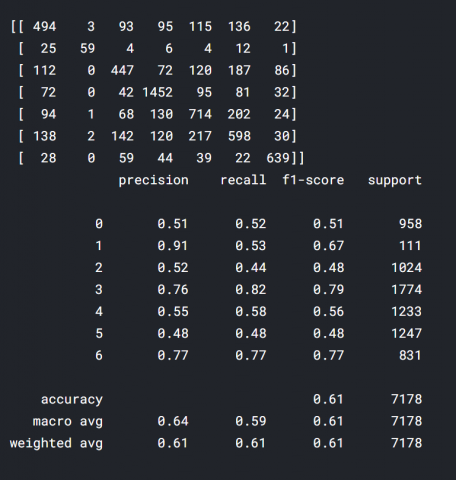
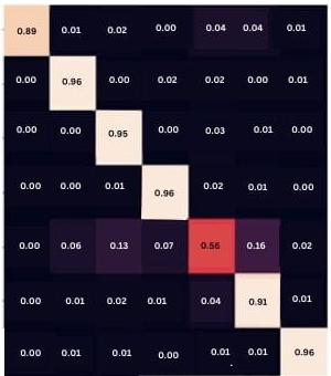
Figure 2(a) represents the resultant values of the confusion matrix and performance metrics when the FER2013 dataset without noise is considered and given for the proposed FERCNN model for evaluation. Whereas in Figure 2(b) represents the respective heat map, from Figure 2(a), it is observed that weighted average accuracy, precision, recall, and F1-score values are 0.61, 0.61, 0.61 & 0.61 respectively.
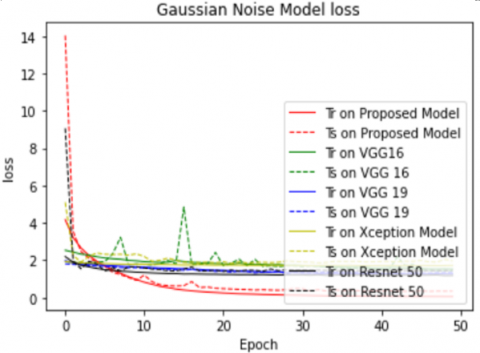
Figures 3 represent FERCNN model accuracy and loss comparisons under various cases such train and test with Gaussian noise, train with Gaussian noise and test without noise, train without noise and test with Gaussian noise and train and test without noise and observed that accuracy has been increased and loss has been decreased when noise is applied to the data and the details of the results are given in Table 2.
Figure 3(c) represents the resultant values of the confusion matrix and performance metrics of the proposed FERCNN model when the FER2013 dataset is injected with Gaussian noise and given for evaluation. Standard deviation and variance parameter values of 8 and 10 are as input to the Gaussian noise function to produce Gaussian noisy images. The proposed FERCNN Model resulted in weighted average accuracy of 0.92, precision of 0.92, recall of 0.92 and F1-score of 0.91 after experimentation where as Figure 3(d) represents the respective heat map of the confusion matrix.
(a) Confusion matrix and performance matrix
(b) Heat map
Figure 2. Performance analysis of FERCNN models on FER2013 dataset without noise
(a) Accuracy comparison
(b) Loss comparison
(c) model confusion matrix
(d) model heat map
Figure 3. Performance comparison of FERCNN model on FER2013 dataset with gaussian noise
Table 2. Performance comparison of different noises in different cases on FER2013
|
S. No |
Noise Applied |
Mode of Training and Testing |
Train Accuracy |
Test Accuracy |
Train Loss |
Test Loss |
Epoch Time |
|
1 |
Gaussian Noise |
Train & Test with Noise |
99.70 |
91.95 |
0.066 |
0.361 |
9 sec |
|
Train Without Noise & Test with Noise |
96.15 |
13.38 |
0.452 |
60.35 |
9 sec |
||
|
Train with Noise & Test Without Noise |
99.41 |
87.27 |
0.079 |
0.606 |
9 sec |
||
|
Train & Test without Noise |
62.37 |
63.61 |
1.113 |
0.636 |
16 sec |
||
|
2 |
Poisson Noise |
Train & Test with Noise |
99.65 |
94.61 |
0.075 |
0.255 |
9 sec |
|
Train Without Noise & Test with Noise |
99.67 |
71.54 |
0.097 |
1.393 |
9 sec |
||
|
Train with Noise & Test Without Noise |
99.64 |
88.68 |
0.085 |
0.414 |
9 sec |
||
|
Train & Test without Noise |
73.90 |
74.75 |
0.864 |
0.874 |
16 sec |
||
|
3 |
Speckle Noise |
Train & Test with Noise |
99.55 |
92.45 |
0.065 |
0.327 |
9 sec |
|
Train Without Noise & Test with Noise |
99.39 |
87.97 |
0.093 |
0.544 |
9 sec |
||
|
Train with Noise & Test Without Noise |
99.49 |
90.85 |
0.064 |
0.370 |
9 sec |
||
|
Train & Test without Noise |
61.06 |
64.36 |
1.128 |
1.058 |
16 sec |
||
|
4 |
Salt & Pepper Noise |
Train & Test with Noise |
99.61 |
87.84 |
0.057 |
0.482 |
9 sec |
|
Train Without Noise & Test with Noise |
97.37 |
34.42 |
0.329 |
4.639 |
9 sec |
||
|
Train with Noise & Test Without Noise |
98.21 |
36.30 |
0.263 |
6.059 |
9 sec |
||
|
Train & Test Without Noise |
62.65 |
64.36 |
1.128 |
1.058 |
16 sec |
(a) Accuracy comparison
(b) Loss comparison
(c) Confusion matrix and performance matrix
(d) Heat map
Figure 4. Analysis of FERCNN model performance on FER2013 dataset with salt & pepper noise
Figures 4(a) and (b) represent FERCNN model accuracy and loss comparisons under various cases such as train and test with Salt & Pepper noise, train Salt & Pepper noise and test without noise, train without noise and test with Salt & Pepper noise and train and test without noises and observed that optimal accuracy and losses were obtained when the model is trained and tested with Salt & Pepper noise when compared to remaining cases. The details of the obtained results are given in Table 2.
Figure 4(c) represents the resultant values of the confusion matrix and performance metrics of the proposed FERCNN model when the FER2013 dataset is injected with Salt& Pepper noise and given for evaluation. The amount of noise added to the images is 5% and the proposed FERCNN model resulted in weighted average accuracy of 0.88, precision of 0.88, recall of 0.88 and F1-score of 0.87 after experimentation with the noisy images, Figure 4(d) represents the respective heat map of the confusion matrix.
Figures 5(a) and (b) represent FERCNN model accuracy and loss comparisons under various cases such train and test with Speckle noise, train with Speckle noise and test without noise, train without noise and test with Speckle noise and train and test without noise and observed that accuracy has been increased and loss has been decreased when noise is applied to the data and the details of the results are given in Table 2.
(a) Accuracy comparison
(b) Loss comparison
(c) Confusion matrix and performance matrix
(d) Heat map
Figure 5. Analysis of FERCNN model performance on FER2013 dataset with speckle noise
(a) Accuracy comparison
(b) Loss comparison
(c) Confusion matrix and performance matrix
(d) Heat map
Figure 6. Analysis of FERCNN model performance on FER2013 dataset with Poisson noise
(a) Accuracy comparison
(b) Loss comparison
Figure 7. Comparison of FERCNN performance with various models on FER2013 dataset injected with gaussian noise
(a) Accuracy comparison
(b) Loss comparison
Figure 8. Comparison of FERCNN performance with various models on FER2013 dataset injected with salt & pepper noise
(a) Accuracy comparison
(b) Loss comparison
Figure 9. Comparison of FERCNN performance with various models on FER2013 dataset injected with speckle noise
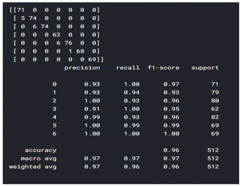
Figure 5(c) represents the resultant values of the confusion matrix and performance metrics of the proposed FERCNN model when the FER2013 dataset is injected with Speckle noise and given for evaluation. Standard deviation, mean and variance parameter values of 20, 05 and 02 are as input to the Speckle noise function to produce Speckle noisy images. The proposed FERCNN Model resulted in weighted average accuracy of 0.92, precision of 0.93, recall of 0.92 and F1-score of 0.92 after experimentation where as Figure 5(d) represents the respective heat map of the confusion matrix.
Figures 6(a) and (b) represent FERCNN model accuracy and Loss comparisons under various cases such train and test with Poisson noise, train with Poisson noise and test without noise, train without noise and test with Poisson noise and train and test without noise and observed that accuracy has been increased and loss has been decreased when Poisson noise is applied to the data and the details of the results are given in Table 2.
(a) Accuracy comparison
(b) Loss comparison
Figure 10. Comparison of FERCNN performance with various models on FER2013 dataset injected with Poisson noise
(a) Without noise
(b) With gaussian noise
(c) With salt & Pepper noise
(d) With Poisson noise
(e) With speckle noise
Figure 11. Confusion matrix and performance matrix of FERCNN Models on JAFFE dataset under various noise conditions
Figure 6(c) represents the resultant values of the confusion matrix and performance metrics of the proposed FERCNN model when the FER2013 dataset is injected with some random Poisson noise and given for evaluation. The proposed FERCNN Model resulted in weighted average accuracy of 0.95, precision of 0.95, recall of 0.95 and F1-score of 0.9 after experimentation where as Figure 6(d) represents the respective heat map of the confusion matrix.
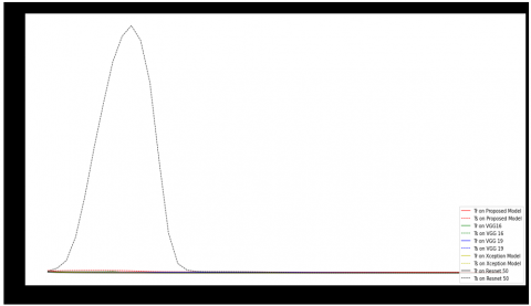
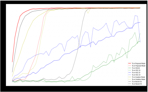
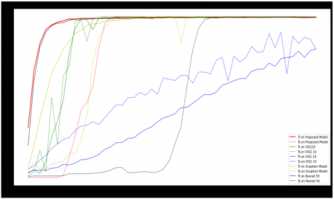
Figure 7(a) represents the Accuracy comparison of the proposed FERCNN model over VGG16, VGG19, Xception and Resnet 50 models in which the FER 2013 dataset is injected with Gaussian noise and given as input to the models for evaluation, Standard deviation and variance of 10 and 8 are used to produce Gaussian noise. It has been observed that the proposed FERCNN model out performed the existing models. Where as in Figure 7(b) represents the Loss comparisons of various models over Proposed FERCNN Model in the same scenario, it is observed that the proposed model loss is minimum when compared to other models. The detailed description of the results is given in Table 3.
Figures 8(a) and (b) represents the accuracy and Loss comparisons of the proposed FERCNN model over VGG16, VGG19, Xception and Resnet50 models in which the FER 2013 dataset is injected with Salt & Pepper noise and given as input to the models for evaluation, 5% of Salt & Pepper noise is injected to the images. It has been observed that the proposed FERCNN models accuracy and loss are better than existing models but not promising. The detailed description of the results are given in Table 3.
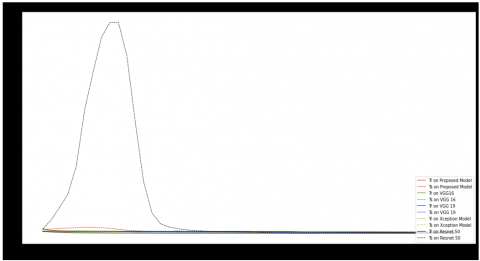
Figure 9(a) represents the Accuracy comparison of the proposed FERCNN model over VGG16, VGG19, Xception and Resnet50 models in which the FER 2013 dataset is injected with Speckle noise and given as input to the models for evaluation, Standard deviation, mean and variance of 10,5 &2 are used to produce Speckle noise. It has been observed that the proposed FERCNN model out performed the existing models. Where as in Figure 9(b) represents the Loss comparisons of various models over the Proposed FERCNN Model in the same scenario, it is observed that the proposed model loss is minimum when compared to other models. The detailed description of the results are given in Table 3.
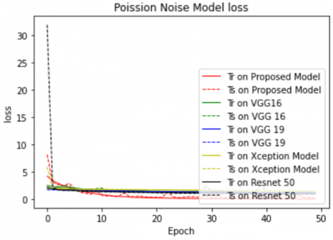
Figure 10(a) represents the Accuracy comparison of the proposed FERCNN model over VGG16, VGG19, Xception and Resnet50 models in which the FER 2013 dataset is injected with some random amount of Poisson noise and given as input to the models for evaluation. It has been observed that the proposed FERCNN model out performed the existing models. Where as in Figure 10(b) represents the Loss comparisons of various models over the Proposed FERCNN Model in the same scenario, it is observed that the proposed model loss is minimum when compared to other models. The detailed description of the results is given in Table 3.
Figure 11 shows the confusion matrix and performance metrics of Proposed FERCNN Model when different kinds of noises are injected on JAFFE dataset and given for evaluation. Figure 11(a) is the case where noise was not injected and observed weighted average accuracy, precision, recall and f1-score values of 0.95, 0.95, 0.95, 0.95 respectively. By injecting Gaussian, Poisson and Speckle noises on JAFFE data sets whose results are shown in Figure 11(b), Figure 11(d), Figure 11(e) resulted in a weighted average accuracy, precision, recall and f1-score values of 1.0,1.0 ,1.0,1.0 which says that the classification accuracy is 100% where as by injecting Salt & Pepper noise whose results are given in Figure 11(c) resulted in a weighted average accuracy, precision, recall and f1-score values of 0.96, 0.97, 0.96, 0.96 achieving a classification accuracy of 96%.
Figure 12 represents the accuracy and Loss comparisons of the proposed FERCNN model over VGG16, VGG19, Xception and Resnet50 models in which the JAFFE dataset is injected with Gaussian noise and given as input to the models for evaluation, Standard deviation and variance of 10 and 8 are used to produce Gaussian noise. It has been observed that all the models except VGG19 produced similar results, where as VGG19 model performance is less when compared to others. The detailed description of the results is given in Table 4.
Figure 13 represents the accuracy and Loss comparisons of the proposed FERCNN model over VGG16, VGG19, Xception and Resnet50 models in which the JAFFE dataset is injected with 5% of Salt & Pepper noise and given as input to the models for evaluation. The performance of all the models is almost similar except for VGG19 whose performance is less when compared to others. The proposed FERCNN model the detailed description of the results is given in Table 4.
Table 3. Performance comparison of various models over proposed FERCNN model on FER2013 dataset
|
S. No |
Type of Noise |
Name of The Model |
Train Accuracy |
Test Accuracy |
Train Loss |
Test Loss |
Epoch Time |
|
1 |
Gaussian Noise |
Proposed FERCNN Model |
99.67 |
92.17 |
0.060 |
0.354 |
10 Sec |
|
VGG 16 |
41.11 |
41.41 |
1.449 |
1.456 |
24 sec |
||
|
VGG 19 |
54.02 |
47.05 |
1.229 |
1.341 |
24 sec |
||
|
Xception |
31.38 |
28.84 |
1.880 |
1.971 |
25 sec |
||
|
Resnet 50 |
58.03 |
45.97 |
1.107 |
1.463 |
25 sec |
||
|
2 |
Salt & Pepper Noise |
Proposed FERCNN Model |
99.61 |
86.94 |
0.057 |
0.528 |
9 sec |
|
VGG 16 |
37.53 |
17.34 |
1.558 |
3.054 |
32 sec |
||
|
VGG 19 |
34.92 |
10.68 |
1.668 |
2.382 |
19 sec |
||
|
Xception |
32.10 |
1051 |
1.682 |
2.402 |
34 sec |
||
|
Resnet 50 |
43.41 |
7.56 |
1.458 |
3.049 |
20 sec |
||
|
3 |
Poisson Noise |
Proposed FERCNN Model |
95.98 |
95.07 |
0.068 |
0.227 |
9 sec |
|
VGG 16 |
47.21 |
47.18 |
1.238 |
1.198 |
20 sec |
||
|
VGG 19 |
55.19 |
56.93 |
1.213 |
1.132 |
22 sec |
||
|
Xception |
41.45 |
45.70 |
1.483 |
1.421 |
23 sec |
||
|
Resnet 50 |
61.27 |
63.97 |
1.029 |
0.639 |
24 sec |
||
|
4 |
Speckle Noise |
Proposed FERCNN Model |
99.54 |
92.41 |
0.060 |
0.343 |
9 sec |
|
VGG 16 |
52.91 |
51.11 |
1.201 |
1.213 |
36 sec |
||
|
VGG 19 |
45.52 |
48.98 |
1.349 |
1.332 |
22 sec |
||
|
Xception |
49.18 |
48.54 |
1.319 |
1.436 |
38 sec |
||
|
Resnet 50 |
55.09 |
54.52 |
1.187 |
1.221 |
23 sec |
(a) Accuracy comparison
(b) Loss comparison
Figure 12. Comparison of FERCNN performance with various models on JAFFE dataset injected with gaussian noise
(a) Accuracy comparison
(b) Loss comparison
Figure 13. Comparison of FERCNN performance with various models on JAFFE dataset injected with salt & pepper noise
(a) Accuracy comparison
(b) Loss comparison
Figure 14. Comparison of FERCNN performance with various models on JAFFE dataset injected with Poisson noise
Figure 15. Accuracy comparison of FERCNN with various models when JAFFE is injected with speckle noise
Table 4. Performance comparison of various models over proposed FERCNN model on JAFFE dataset
|
S.No |
Type of Noise |
Name of The Model |
Train Accuracy |
Test Accuracy |
Train Loss |
Test Loss |
Epoch Time |
|
1 |
Gaussian Noise |
Proposed FERCNN Model |
99.80 |
100 |
0.021 |
0.004 |
1 sec |
|
VGG 16 |
99.80 |
100 |
0.021 |
0.004 |
2 sec |
||
|
VGG 19 |
86.13 |
76.37 |
0.465 |
0.664 |
2 sec |
||
|
Xception |
99.90 |
100 |
0.013 |
0.005 |
11 sec |
||
|
Resnet 50 |
99.78 |
100 |
0.032 |
0.004 |
2 sec |
||
|
2 |
Salt & Pepper Noise |
Proposed FERCNN Model |
99.85 |
100 |
1.456 |
1.429 |
1 sec |
|
VGG 16 |
59.65 |
70.31 |
1.048 |
0.863 |
2 sec |
||
|
VGG 19 |
82.64 |
59.39 |
0.560 |
1.069 |
2 sec |
||
|
Xception |
99.70 |
99.80 |
0.021 |
0.011 |
11 se |
||
|
Resnet 50 |
99.68 |
99.22 |
0.049 |
0.449 |
2 sec |
||
|
3 |
Poisson Noise |
Proposed FERCNN Model |
99.81 |
100 |
1.226 |
1.199 |
1 sec |
|
VGG 16 |
99.70 |
100 |
0.018 |
0.012 |
2 sec |
||
|
VGG 19 |
80.63 |
82.42 |
0.572 |
0.563 |
2 sec |
||
|
Xception |
99.92 |
100 |
0.010 |
0.003 |
11 sec |
||
|
Resnet 50 |
99.65 |
99.80 |
0.044 |
0.011 |
2 sec |
||
|
4 |
Speckle Noise |
Proposed FERCNN Model |
99.89 |
99.61 |
1.387 |
1.414 |
1 sec |
|
VGG 16 |
99.86 |
99.61 |
0.025 |
0.044 |
2 sec |
||
|
VGG 19 |
86.58 |
95.12 |
0.464 |
0.356 |
2 sec |
||
|
Xception |
99.81 |
99.61 |
0.019 |
0.037 |
11 sec |
||
|
Resnet 50 |
99.83 |
99.61 |
0.032 |
0.027 |
2 sec |
Figure 14 represents the accuracy and Loss comparisons of the proposed FERCNN model over VGG16, VGG19, Xception and Resnet50 models in which the JAFFE dataset is injected with some random amount of Poisson noise and given as input to the models for evaluation. The performance of all the models are almost similar except VGG19 whose performance is not as good as other models. The details of the results are given in Table 4
Figure 15 represents the accuracy and Loss comparisons of the proposed FERCNN model over VGG16, VGG19, Xception and Resnet50 models in which the JAFFE dataset is injected with Speckle noise and given as input to the models for evaluation, Standard deviation, mean and variance of 10,5 & 2 are used to produce Speckle noise. It has been observed that the performance of all the models is almost similar with slight variations.
An observation from Figure 12 to Figure 15 and Table 4 was that the time taken for each epoch by proposed FERCNN Model is 1Sec, VGG16, VGG19 and Resnet50 models is 2Sec and Xception model is 11Sec which says that the time taken for execution is less for the proposed model when compared to other models.
The experiments conducted on the stated hypothesis are justifying the performance in place of noisy input. In the proposed experimental setup, the training and validation of the model with noisy images stood with high accuracy than non-noisy images. It has been noticed that training and testing accuracies with Gaussian, Poisson, Speckle, Salt & pepper varies in between 99.55 to 99.70 and 87.84 to 94.61 whereas without injecting noise varies in between 61.06 to 73.9 and 63.61 to 74.75. The differences of classifying emotions with respect to noisy and non-noisy varies between 25.75 to 38.49 for training and 19.86 to 28.34 for testing. This proves the hypothesis that model buildup with noise is more efficient than without injecting noise. It is also witnessed that the epoch time which is needed to tune the parameters of the network is lower in case of injected input noise to non-noise images. The epoch time with noise took 9 seconds whereas in the latter case it is 16 seconds on an average, this indicates injected noise images model training is 1.77 times faster than the others. It has been noticed that the performance achieved by the FERCNN model is higher than the predefined popular CNN architectures like VGG16, VGG19, Xception, Resnet50 subject to condition if the dataset contains a large number of images and marginally equivalent if the dataset contains a small number of images. The epoch time obtained is 9 to 10 Seconds for FERCNN model whereas it is 22.25 to 29.75 Seconds for other discussed CNN models. It seems the proposed FERCNN model is not only a better choice in terms of accuracy but also model training and evaluation time. Facial emotion classification is important in a variety of applications, including education, customer satisfaction, detecting driver fatigue, and many more. In some circumstances, the input photos may not be clear enough to make necessary conclusions. Because our model was built for categorizing photos with noise, it will be effective in delivering superior results when compared to others who utilize this application. The method employed in the current study can be used to model parameters like weights, and comparison analysis can be performed, which will be a part of the future work. In the current work, noise was only introduced at the input level of the images.
[1] Padmapriya, S., KalaJames, E.A. (2012). Real time smart car lock security system using face detection and recognition. In 2012 International Conference on Computer Communication and Informatics, IEEE, pp. 1-6. https://doi.org/10.1109/ICCCI.2012.6158802
[2] Xu, Z., Hu, C., Mei, L. (2016). Video structured description technology based intelligence analysis of surveillance videos for public security applications. Multimedia Tools and Applications, 75: 12155-12172. https://doi.org/10.1007/s11042-015-3112-5
[3] Yan, Z., Xu, Z., Dai, J. (2017). The big data analysis on the camera-based face image in surveillance cameras. Intelligent Automation & Soft Computing, 1-9. https://doi.org/10.1080/10798587.2016.1267251
[4] McAllister, D. (2007). Law enforcement turns to face-recognition technology. Information Today, 24(5): 50-52.
[5] McKenna, S.J., Gong, S. (1997). Non-intrusive person authentication for access control by visual tracking and face recognition. In International Conference on Audio-and Video-Based Biometric Person Authentication. Berlin, Heidelberg: Springer Berlin Heidelberg, pp. 177-183. https://doi.org/10.1007/BFb0015994
[6] Xu, J., Zhang, K., Xu, M., Zhou, Z. (2009). An adaptive threshold method for image denoising based on wavelet domain. In MIPPR 2009: Automatic Target Recognition and Image Analysis. SPIE, 7495: 1194-1200. https://doi.org/10.1117/12.831402
[7] Ahonen, T., Pietikäinen, M. (2007). Soft histograms for local binary patterns. In Proceedings of the Finnish Signal Processing Symposium, FINSIG, 5(9): 1.
[8] Ren, J., Jiang, X., Yuan, J. (2015). LBP encoding schemes jointly utilizing the information of current bit and other LBP bits. IEEE Signal Processing Letters, 22(12): 2373-2377. https://doi.org/10.1109/LSP.2015.2481435
[9] Gulcehre, C., Moczulski, M., Denil, M., Bengio, Y. (2016). Noisy activation functions. In International Conference on Machine Learning. PMLR, pp. 3059-3068.
[10] Sietsma, J., Dow, R.J. (1991). Creating artificial neural networks that generalize. Neural Networks, 4(1): 67-79. https://doi.org/10.1016/0893-6080(91)90033-2
[11] Schmidhuber, J. (2015). Deep learning in neural networks: An overview. Neural Networks, 61: 85-117. https://doi.org/10.1016/j.neunet.2014.09.003
[12] Alonso-Weber, J.M., Sesmero, M.P., Sanchis, A. (2014). Combining additive input noise annealing and pattern transformations for improved handwritten character recognition. Expert Systems With Applications, 41(18): 8180-8188. https://doi.org/10.1016/j.eswa.2014.07.016
[13] Baldi, P., Sadowski, P. (2014). The dropout learning algorithm. Artificial Intelligence, 210: 78-122. https://doi.org/10.1016/j.artint.2014.02.004
[14] An, G. (1996). The effects of adding noise during backpropagation training on a generalization performance. Neural Computation, 8(3): 643-674. https://doi.org/10.1162/neco.1996.8.3.643
[15] Neelakantan, A., Vilnis, L., Le, Q.V., Sutskever, I., Kaiser, L., Kurach, K., Martens, J. (2015). Adding gradient noise improves learning for very deep networks. arXiv Preprint arXiv: 1511.06807. https://doi.org/10.48550/arXiv.1511.06807
[16] Poole, B., Sohl-Dickstein, J., Ganguli, S. (2014). Analyzing noise in autoencoders and deep networks. arXiv Preprint arXiv: 1406.1831. https://doi.org/10.48550/arXiv.1406.1831
[17] Zhang, B., Shan, S., Chen, X., Gao, W. (2006). Histogram of gabor phase patterns (HGPP): A novel object representation approach for face recognition. IEEE Transactions on Image Processing, 16(1): 57-68. https://doi.org/10.1109/TIP.2006.884956
[18] Chen, L., Zhou, M., Su, W., Wu, M., She, J., Hirota, K. (2018). Softmax regression based deep sparse autoencoder network for facial emotion recognition in human-robot interaction. Information Sciences, 428: 49-61. https://doi.org/10.1016/j.ins.2017.10.044
[19] Guo, Z., Zhang, L., Zhang, D. (2010). Rotation invariant texture classification using LBP variance (LBPV) with global matching. Pattern Recognition, 43(3): 706-719. https://doi.org/10.1016/j.patcog.2009.08.017
[20] Chang, W.Y., Hsu, S.H., Chien, J.H. (2017). FATAUVA-Net: An integrated deep learning framework for facial attribute recognition, action unit detection, and valence-arousal estimation. In Proceedings of the IEEE Conference on Computer Vision and Pattern Recognition Workshops, pp. 17-25. https://doi.org/10.1109/CVPRW.2017.246
[21] Ly, S.T., Lee, G.S., Kim, S.H., Yang, H.J. (2018). Emotion recognition via body gesture: Deep learning model coupled with keyframe selection. In Proceedings of the 2018 International Conference on Machine Learning and Machine Intelligence, pp. 27-31. https://doi.org/10.1145/3278312.3278313
[22] Kaya, H., Gürpınar, F., Salah, A.A. (2017). Video-based emotion recognition in the wild using deep transfer learning and score fusion. Image and Vision Computing, 65: 66-75. https://doi.org/10.1016/j.imavis.2017.01.012
[23] Mohammed, M., Sowmya, M.V.S., Akhila, Y., Megana, B.N. (2019). Visual modeling of data using convolutional neural networks. International Journal of Engineering and Advanced Technology (IJEAT) ISSN, 2249-8958.
[24] Kishore, P.V.V., Kumar, K.V.V., Kiran Kumar, E., Sastry, A.S.C.S., Teja Kiran, M., Anil Kumar, D., Prasad, M.V.D. (2018). Indian classical dance action identification and classification with convolutional neural networks. Advances in Multimedia, 2018. https://doi.org/10.1155/2018/5141402
[25] Mohammed, M., Nalluru, S.S., Tadi, S., Samineni, R. (2019). Brain tumor image classification using convolutional neural networks. International Journal of Advanced Science and Technology, 29(5): 928-934.
[26] Praveena, M., Rohini, G., Reddy, G.T., Nikhil, K.H.S. (2019). Automatic brain tumor identification using clustering of k-means algorithm in image processing. Journal of Advanced Research in Dynamical and Control Systems, 11(7): 621-630.
[27] Pradeepini, G., Babu, B.S., Tejaswini, T., Priyanka, D., Harshitha, M. (2018). A comparative study on brain tumor diagnosis techniques using MRI image processing. International Journal of Engineering and Technology, 7(32): 486-489.
[28] Vamsidhar, E., Rani, P.J., Babu, K.R. (2019). Plant disease identification and classification using image processing. International Journal of Engineering and Advanced Technology, 8(3): 442-446.
[29] Lakshmi, P., Vidyullatha, P. (2019). Automated leaf disease detection in corn species through image analysis. International Journal of Advanced Trends in Computer Science and Engineering, 8(6): 2893-2899.
[30] Ramya Keerthi, P., Niharika, B., Dinesh Kumar, G., Sai Venakat, K., Sheela Rani, C.M. (2019). Reorganization of license plate characteristics using image processing techniques. International Journal of Recent Technology and Engineering, 7(6): 1260-1264.
[31] Inthiyaz, S., Madhav, B.T.P., Kishore, P.V.V. (2018). Flower image segmentation with PCA fused colored covariance and gabor texture features based level sets. Ain Shams Engineering Journal, 9(4): 3277-3291. https://doi.org/10.1016/j.asej.2017.12.007
[32] Liu, C. (2004). Gabor-based kernel PCA with fractional power polynomial models for face recognition. IEEE Transactions on Pattern Analysis and Machine Intelligence, 26(5): 572-581. https://doi.org/10.1109/TPAMI.2004.1273927
[33] Lan, R.S., Lu, H.M., Zhou, Y.C., Liu, Z.B., Luo, X.N. (2020). An LBP encoding scheme jointly using quaternionic representation and angular information. Neural Comput & Applic, 32: 4317-4323. https://doi.org/10.1007/s00521-018-03968-y
[34] Ahonen, T., Hadid, A., Pietikainen, M. (2006). Face description with local binary patterns: Application to face recognition. IEEE Transactions on Pattern Analysis and Machine Intelligence, 28(12): 2037-2041. https://doi.org/10.1109/TPAMI.2006.244
[35] Abdulrahman, M., Gwadabe, T.R., Abdu, F.J., Eleyan, A. (2014). Gabor wavelet transform based facial expression recognition using PCA and LBP. In 2014 22nd Signal Processing and Communications Applications Conference (SIU), IEEE, pp. 2265-2268. https://doi.org/10.1109/SIU.2014.6830717
[36] OpenAI. Better Exploration with Parameter Noise. https://blog.openai.com/better-exploration-with-parameter-noise/
[37] Kavitha, K., Rao, B.T. (2019). Evaluation of distance measures for feature based image registration using alexnet. arXiv Preprint arXiv: 1907.12921. https://doi.org/10.14569/IJACSA.2018.091034
[38] Alkaddour, M., Tariq, U. (2020). Investigating the effect of noise on facial expression recognition. In Advances in Computer Vision: Proceedings of the 2019 Computer Vision Conference (CVC). Springer International Publishing, 2(1): 699-709. https://doi.org/10.1007/978-3-030-17798-0_55
[39] Mahmood, A., Hussain, S., Iqbal, K., Elkilani, W.S. (2019). Recognition of facial expressions under varying conditions using dual-feature fusion. Mathematical Problems in Engineering, 2019. https://doi.org/10.1155/2019/9185481
[40] Abd, R.G., Ibrahim, A.W.S., Noor, A.A. (2023). Facial emotion recognition using HOG and convolution neural network. Ingénierie des Systèmes d’Information, 28(1): 169-174. https://doi.org/10.18280/isi.280118
[41] Al-Atroshi, S.J.A., Ali, A.M. (2023). Improving facial expression recognition using HOG with SVM and modified datasets classified by Alexnet. Traitement du Signal, 40(4): 1611-1619. https://doi.org/10.18280/ts.400429