Zainab Ali Abd Alhuseen*![]() | Fanar Ali Joda
| Fanar Ali Joda![]() | Mohammed Abdullah Naser
| Mohammed Abdullah Naser![]()
© 2023 IIETA. This article is published by IIETA and is licensed under the CC BY 4.0 license (http://creativecommons.org/licenses/by/4.0/).
OPEN ACCESS
The focus of this study encompasses the burgeoning field of abnormal behavior detection through computer vision, with a specific emphasis on gait analysis. A foundational gait model has been constructed, deriving from an extensive analysis of various gait types. The research endeavors to establish a model capable of discerning individual abnormal behavior, predicated on their walking patterns. A meticulous evaluation and comparison of three predominant feature extraction methodologies—Histogram of Oriented Gradients (HOG), Local Binary Pattern (LBP), and Center Symmetric Local Binary Pattern (CS-LBP)—constitute the core of this study. These techniques have been selected owing to their prevalent application and validated efficacy across numerous computer vision domains. Following feature extraction, the classification stage is initiated, utilizing Convolutional Neural Networks (CNNs), a paradigm of deep learning algorithms. The methodology has undergone rigorous testing and evaluation on a comprehensive dataset, inclusive of both standard and aberrant behavioral instances. A high performance level, signified by a 99% accuracy rate, was achieved through the application of the CS-LBP method for abnormal behavior detection. The empirical results underscore the significance of gait feature extraction methods in augmenting the system’s proficiency in anomaly detection.
abnormal behavior detection, gait analysis, deep learning, feature extraction, local spatial features, Center Symmetric Local Binary Pattern (CS-LBP), Convolutional Neural Network (CNN)
In contemporary society, the significance of public security visual monitoring is escalating. The proliferation of video surveillance data necessitates the development of automated visual monitoring systems capable of detecting abnormal behaviors. Individuals deviating from typical walking patterns are identified as exhibiting abnormal behavior, which is defined by psychologists as actions diverging from the standard, typical, or stereotyped [1].
Gait, a biometric characteristic, holds potential for individual identification based on walking patterns, yet it demands a robust security system within the current technological landscape. The field of human gait analysis is emerging in computer vision, boasting substantial applications in medical diagnosis, such as osteoporosis, and patient monitoring [2]. The challenge of anomaly detection in video data involves the identification, classification, tracking, and recognition of object behavior, aiming to maintain vigilant observation in collected footage. Despite numerous methodologies proposed by researchers, the quest for a flawless video surveillance system remains unfulfilled.
The objective of discerning objects, events, and behaviors within video sequences has been a longstanding pursuit in video surveillance. Automatic video surveillance systems, with their heightened security and augmented monitoring capabilities, are integral in safeguarding public spaces such as banks, retail centers, metro stations, airports, military installations, and other densely populated areas. These systems play a pivotal role in fortifying security measures, diminishing response times, and yielding critical insights to inform decision-making across various public domains and strategic locations. The paramount aim of video surveillance lies in the accurate identification, classification, and detection of anomalous behaviors and patterns, subsequently categorized as “suspicious” [3].
A necessity has arisen for an automated system capable of discerning violent behavior through the analysis of individuals' gait patterns, leveraging deep learning techniques. This requirement stems from the inefficiencies of human operators in scrutinizing surveillance footage, a delay that can lead to detrimental outcomes, including property damage and personal injuries [4].
Addressing the limitations of human operators in monitoring surveillance footage, an automated system utilizing deep learning techniques, specifically CNN, is necessitated. This system, focusing on gait-based anomaly detection, employs local spatial feature extraction methods to accurately identify individuals exhibiting abnormal gait patterns.
The remaining sections of this document are structured as follows: Related works are reviewed in Section 2, while Section 3 elucidates the methodology of feature extraction. The proposed system is introduced in Section 4. Section 5 presents and discusses the obtained results, and the study is concluded in Section 6.
The utilization of computer vision for the detection of anomalies in human gait has been extensively researched and developed, underscoring its critical importance in applications spanning healthcare and security. This section encapsulates a synopsis of select literature pivotal to this domain.
In 2016, a novel approach to gait recognition was proposed by Shiraga et al. [5], employing a CNN architecture . The gait energy image (GEI), serving as an image-based representation of gait, was introduced as the input to a specifically designed CNN for gait recognition, denominated as GEINet. Comprising two sequences of convolution, pooling, and normalization layers, followed by two fully connected layers, GEINet was meticulously crafted to yield a set of similarities across diverse subjects in the training dataset. The efficacy of this approach was rigorously evaluated on the OU-ISIR dataset, encompassing a substantial population in both cooperative and non-cooperative scenarios.
In the realm of gait analysis utilizing sensor technologies, a pivotal study was conducted by Gao et al. [6] in 2019, where a wearable inertial measurement unit (IMU) was employed to discern aberrant gait patterns, including threshold walking, tiptoeing, and hemiplegic walking . A novel application of long short-term memory and CNN (LSTM-CNN) technologies was proposed for the identification and classification of these anomalous gaits. Enhancements were made to the convergence layer of the LSTM-CNN model, augmenting its capacity to categorize aberrant gait patterns effectively. The LCWSnet-based methodology, as elucidated in their findings, demonstrated proficiency in anomaly detection within gait data.
Subsequently, in 2020, a comprehensive study by Khan et al. [7] addressed the presence of individuals exhibiting suspected aberrant behaviors, particularly in their walking styles . They advocated for the integration of robust deep learning clustering features into a Kernel Extreme Learning Machine, presenting a multi-faceted framework. Initially, transfer learning was applied to retrain two pre-existing CNN models on general walking datasets, from which features of the fully connected layer were extracted. A novel probabilistic method, termed Euclidean Norm and Geometric Mean Maximization with Conditional Entropy, was then employed to discern the most salient features. Canonical correlation analysis was utilized to compile robust features, culminating in the classification of various gait patterns through a series of sieves. The effectiveness of the proposed framework was validated on the publicly available gait image dataset, CASIA B.
In a scholarly investigation conducted in 2022, Kuppusamy and Bharathi [8] explored the application of various CNNs for the identification of anomalous human activities within video footage . It was elucidated in the study that three-dimensional CNNs exhibit superior efficacy in executing machine learning algorithms. A comparative analysis was undertaken, revealing the formulation of several CNN models, each meticulously crafted to discern a range of aberrant human behaviors across diverse datasets.
Furthermore, Jameel and Dhannoon, in their 2022 work, meticulously delineated a process for ascertaining an individual's identity through the analysis of their gait, captured in video format [2]. The video undergoes a sequential transformation, initiated by the conversion of each frame to a grayscale format, followed by the meticulous removal of all superfluous elements and noise. Subsequent steps involve the identification of motion through the comparison of consecutive frames, conversion of the results into a binary image, and the application of morphological operations. The culmination of this process is the classification phase, underpinned by a deep neural network, representing the most critical stage of the system.
In the methodology section, a mathematical approach is employed to represent millions of numeric pixel values through feature vectors, facilitating the interpretation of image patterns by deep learning algorithms. The process of feature extraction is implemented to reduce the dimensionality of the data set, with the objective of deriving a more compact set of features that encapsulates the majority of the information present in the original feature set. Consequently, the initial array of characteristics is condensed to a size that is more amenable to analysis. Among the diverse methodologies available for feature extraction, Local Spatial Feature Extraction (LSFE) methods are utilized. Subsequent to the optimization of the image and its conversion to a grayscale format, the application of local descriptors is rendered more efficacious, thereby enhancing the interpretability of the image. Feature extraction at the pixel level is conducted employing the HOG approach, followed by a secondary phase of feature extraction at the block level, utilizing the LBP and CS-LBP methods.
3.1 Extract features at the pixel level
Feature extraction at the pixel level necessitates the meticulous analysis and transformation of singular pixels or minor pixel conglomerates within an image, aiming to encapsulate pertinent data for subsequent processing and analytical procedures. This stage holds critical importance in the domains of computer vision and image processing. During this process, features are extracted at the pixel level, resulting in an output value at a specific coordinate that is exclusively determined by the input value at the corresponding location.
• HOG
HOG is a feature descriptor initially introduced for the purpose of pedestrian detection [9]. It operates by quantifying the occurrence of gradient directions within a specified detection window, also referred to as a cell. This cell is a compact, rectangular segment of the image designated for the computation of HOG features. The dimensions of this window are variable, and it may share overlapping boundaries with adjacent windows. The procedure involves segmenting the image into an array of these small cells, followed by the calculation of gradient direction histograms for each individual cell. Subsequently, these histograms are concatenated to construct a feature vector, which serves as a basis for image classification. The ensuing discourse encapsulates the fundamental stages involved in the computation of HOG features [10].
- Gradient calculation: In this step, spatial gradients are calculated in the horizontal and vertical directions. These two gradations are then used to calculate the magnitudes and angles of the gradient, as in Eq. (1) and Eq. (2).
$G x=I(x+1, y)-I(x-1, y)$ (1)
$G_y=I(x, y+1)-I(x, y-1)$ (2)
where, Gx and Gy represent the gradient components along the horizontal and vertical directions, respectively. It is noteworthy that convolution of images with the Sobel mask facilitates the computation of these gradient components, as expressed in Eqs. (1) and (2). Subsequently, the size and direction of the gradient can be determined utilizing Eqs. (3) and (4), providing a comprehensive analysis of the image’s features.
$M=\left|G_x\right|+\left|G_y\right|$ (3)
$\theta(x, y)=\tan ^{-1}\left(\frac{G_y}{G_x}\right)$ (4)
where, m= magnitude and θ(x,y) = the direction of the gradient.
- Orientation Binning: In this stage, the image undergoes segmentation into small, contiguous regions termed as cells. Within each cell, the gradient magnitude of individual pixels is allocated across various orientation bins, guided by the corresponding gradient angles. The essence of this binning process is to discretize the gradient orientations, culminating in a representation akin to a histogram.
- Subsequently, the procedure entails aggregating adjacent cells to form blocks, followed by normalization of each individual block. The aggregation and normalization processes facilitate the concatenation of normalized block histograms within a detection window, thereby yielding a comprehensive descriptor.
3.2 Extract features at the block level
The extraction of features at the block level entails meticulous analysis, capturing distinct attributes or characteristics of data within defined blocks or segments. This approach is prevalent across diverse domains, including signal processing, image analysis, and natural language processing. In this context, the features are extracted in such a manner that the output value at a specific coordinate is contingent upon the input values surrounding that particular coordinate.
• LBP
LBP initially introduced by Ojala et al. [11], stands out as a powerful method for texture description, rooted in statistical analysis and proving its efficacy in this domain. Although various adaptations of LBP have been prevalently applied to face analysis due to their superior classification capabilities, their compactness remains yet to be conclusively established. Consequently, the integration of features emerges as a promising strategy. Particularly, the LBP variant that maximizes mutual information has demonstrated enhanced performance in face analysis [12].
The computation of LBP involves a comparative analysis of the gray-level intensity between a central pixel and its adjacent neighbors. Each neighboring pixel is assigned a binary value, determined by whether its intensity surpasses that of the central pixel. Subsequently, these binary values are amalgamated, culminating in a binary pattern which serves as a distinctive image feature. Eqs. (5) and (6) can be employed to articulate the computation and representation of the LBP results [13].
$L B P_{P, R}\left(x_c, y_c\right)=\sum_{n=0}^7 \delta\left(g_n-g_c\right)^{2^n}$ (5)
where, gc represents the value of the central pixel, located at the coordinates (xc, yc), whereas gndenotes the value of one of the eight adjacent pixels surrounding the central pixel, all within a radius R. The total number of pixels in the neighborhood is denoted by P. Furthermore, the function δ(.) is defined as a sign function and its expression is:
$\delta(x) \begin{cases}1 & \text { if } x \geq 0 \\ 0 & \text { otherwise }\end{cases}$ (6)
• CS-LBP
CS-LBP serves as a refined iteration of the traditional LBP. Originally introduced to address certain limitations inherent to the standard LBP [14], the CS-LBP introduces a novel approach wherein the center symmetric pairs of pixels undergo comparison, as opposed to evaluating the gray levels of individual pixels in relation to the center pixel. This method exhibits a strong correlation with gradient operators, encapsulating differences in gray levels among adjacent pairs of pixels within a specified neighborhood. Consequently, CS-LBP harnesses the strengths of both gradient-based features and LBP, effectively capturing prominent textures and edges within the image. The computation of CS-LBP features is governed by Eqs. (7) and (8).
$C S-L B P_{p, r, t}=\sum_{i=0}^{N / 2-1} S\left(\left|g_i-g_{i+N / 2}\right|\right) 2^i$ (7)
$S(x)\left\{\begin{array}{lr}1 & \text { if } x \geq t \\ 0 & \text { otherwise }\end{array}\right.$ (8)
where, gi and g(i+N)⁄2 represent the grayscale values of N centrally symmetric pairs of pixels, which are evenly distributed along the circumference of a circle with radius r. The CS-LBP method uniquely focuses on the differences in grayscale values between opposing pairs of pixels within its defined neighborhood, capturing nuanced variations and patterns.
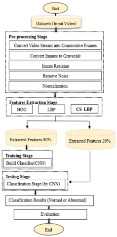
The design of any system is pivotal, delineating its operational mechanisms and outlining the requisite steps to meet specified requirements. In this context, the system under discussion has been engineered to classify behaviors based on an individual’s walking pattern, employing a dataset comprised of collected images to train a classifier for the detection of anomalous behavior. Sequential classifier construction for this behavior identification system is meticulously depicted in Figure 1, which illustrates the critical stages of the proposed system.
4.1 Dataset
The paucity of task-specific datasets, encompassing both public and commercial solutions, constrains the development of new Artificial Intelligence (AI) models designed for human identification based on gait analysis. The dataset under consideration has been manually compiled, encompassing a diverse collection of videos illustrating the walking patterns of two distinct demographic groups: individuals exhibiting typical gait patterns indicative of good health, and individuals diagnosed with various medical conditions resulting in atypical gait patterns. A meticulous manual process was employed for data collection, involving the selection and extraction of video content from various online platforms. These platforms provided access to an array of videos depicting diverse gait scenarios.
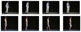
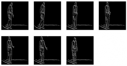
The dataset comprises 112 videos, of which 53 depict individuals demonstrating "normal" gait patterns and 59 depict individuals with "abnormal" gait patterns. In the context of this study, "normal" gait patterns are defined as those associated with individuals free from medical conditions affecting their walking style. Conversely, "abnormal" gait patterns are characterized by deviations from standard walking patterns, potentially resulting from a myriad of factors including, but not limited to, musculoskeletal disorders, neurological impairments, injuries, or other medical conditions impacting motor control. Manifestations of "abnormal" gaits may encompass limping, shuffling, irregular step patterns, or any discernible deviations from conventional gait patterns. A segment of the dataset is visually represented in Figure 2.
Figure 1. Critical stages of the proposed system
Figure 2. Top row containing four frames show abnormal behavior and frames in bottom row show normal behaviour
4.2 Pre-processing
The pre-treatment stage holds paramount importance in the development of a detection system for abnormal gait-based behavior analysis. In preparation for the training phase and the initiation of feature extraction, the dataset undergoes a comprehensive pre-treatment process.
Initially, videos within the dataset are meticulously decomposed into a series of images, commonly referred to as frames. Each frame is subsequently subjected to a multi-stage pre-processing procedure, prior to undergoing classification.
The dimensions of each image are standardized to a resolution of 244*244 pixels. Concurrently, extraneous elements and noise present within the images are meticulously removed to enhance clarity.
Subsequent to these steps, each image is converted to a grayscale format. This conversion is imperative for reducing computational complexity and enhancing the efficiency of the subsequent processing stages.
Finally, a normalization process is applied to the dataset. This is achieved by dividing the pixel values of each image by 255, a step crucial for scaling the data to a range that is conducive to the training of machine learning models.
• Step 1: Convert video stream into consecutive frames
Individuals can be recognized based on their distinctive walking patterns, captured using a digital camera. Once the video footage is segmented into a series of images, referred to as frames, it undergoes processing through various stages.
• Step 2: Convert images into grayscale
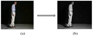
In preparation for subsequent processing, the frames derived from video footage necessitate meticulous preparation and enhancement to eliminate any extraneous content. Initially represented by three-dimensional RGB bands, the images must undergo conversion to a grayscale format, thereby reducing the image graph data channels from three to one and resulting in a two-dimensional grayscale image graph. This transformation facilitates a more swift and efficient execution of the verification process. The aforementioned process and its implications are visually represented in Figure 3.
Figure 3. Images converting to Grayscale (a) RGB image (b) Grayscale image
• Step 3: Dimensionality standardization of images
For the provision of images to a range of predetermined AI algorithms, a uniform dimensionality has been mandated, given the substantial size variations in images captured via camera. A reduction to a dimensionality of (244*244) pixels has been instituted for all images. This specific dimensionality selection aligns with the architectural prerequisites of certain CNN, such as VGG16, which necessitate a consistent input size to operate optimally. Larger image dimensions incur augmented computational demands during both the training and inference phases, attributable to the escalated pixel quantity. The adoption of a (244*244) pixel dimensionality represents a judicious compromise, ensuring the retention of critical image details whilst optimizing computational efficiency, thereby facilitating a more expedited model training process.
• Step 4: Remove noise
Noise intrusion is an inevitable aspect of image acquisition and transmission, necessitating the implementation of image optimization as a vital and integral component of image processing. This stage is instrumental in augmenting the luminance and definition of the images, while simultaneously reducing the noise levels. In lieu of the standard bilinear interpolation, which typically engages a 2*2 pixel neighborhood, this study opts for bicubic interpolation, a more sophisticated method, analyzing a 4*4 pixel neighborhood, thereby incorporating 16 pixels. For the computation of interpolated pixel values across this 4x4 matrix, reference is made to Eq. (9).
$P(x, y)=\sum_{i=0}^3 \sum_{j=0}^3 a_{i j} x^i y^j$ (9)
To address the interpolation challenge, it is imperative to ascertain the 16 coefficients denoted as aij. These coefficients can be derived through the application of partial derivatives to the discrete pixel values, coupled with the p(x, y) values extracted from the pixel matrix. Following the computation of these coefficients, they are then employed to multiply the weights of the known pixels, facilitating the interpolation of the unknown pixel values. Subsequently, the input is subjected to a duplication process. Thereafter, the resizing function is invoked once more, this time incorporating the cv2.INTER_CUBIC interpolation flag, to execute the interpolation utilizing the cv2.
• Step 5: Normalization
The normalization of images represents an essential step in image pre-processing, given that CNNs are calibrated to interpret and process image data within the numerical confines of [0-1]. To align with these operational parameters, a rescaling procedure is applied to each pixel value, transitioning from the initial range of [0-255] to the target range of [0-1]. This rescaling is achieved through division by 255, ensuring compatibility with the CNN’s processing framework.
Refer to Eq. (10) for a comprehensive representation of the data normalization process, where the min() and max() functions denote the extremities of potential values that the data type can accommodate.
$X_i=\frac{X_i-\min (X)}{\max (X)-\min (X)}$ (10)
In the context of image processing, the variable x denotes the entirety of the image, while i signifies an individual pixel within that image. In scenarios involving an 8-bit image, the min() and max() values are correspondingly adjusted to 0 and 255. To facilitate the conversion of an 8-bit image to a floating-point representation, a straightforward division by 255 is employed, particularly when the min() value is in proximity to 0.
4.3 Feature extraction
In image pattern recognition, numerical representations of millions of pixel values are transmuted into feature vectors, a crucial process for facilitating deep learning algorithms' comprehension of image patterns.
The extraction of distinctive features stands as a pivotal component in any pattern recognition system, with the simplification of classification tasks being directly proportional to the quantity and uniqueness of features extracted. Post the image optimization and grayscale conversion processes, the subsequent challenge lies in the selection and extraction of pivotal features, instrumental in achieving accurate classification results.
The extraction of irrelevant feature information from the original frames has been observed to exert an influence on both the system's accuracy and computational efficiency. Additionally, the choice of feature extraction methodologies plays a significant role in influencing the overall performance of the model.
In the system proposed herein, specific methods including HOG, LBP, and CS-LBP have been employed for the extraction of features. These methods have demonstrated proficiency in capturing a diverse array of visual information, encompassing gradients, textures, and symmetrical patterns, all of which are integral to tasks involving object detection and recognition.
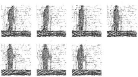
Figure 4. Visual representation of features extracted via HOG method
Figure 5. Visual representation of features extracted via LBP method
Figure 6. Visual representation of features extracted via CS-LBP method
The proposed system utilizes a selection of local descriptor methods for feature extraction. Initially, the HOG method, accompanied by a Sobel mask, is employed. This technique facilitates the generation of images rich in features, as exemplified in Figure 4.
Subsequently, the LBP method was employed, revealing a discernible enhancement in the definition of the extracted features. This augmentation in feature clarity subsequently yielded a positive impact on the accuracy of classification, as demonstrated in the results presented in Figure 5.
Next, the CS-LBP method, a refined variant of the LBP, was implemented on the images. This approach yielded superior results relative to the preceding two methods, as illustrated in Figure 6.
4.4 CNN classifier
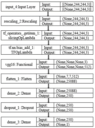
In contemporary computational systems, a paradigm shift has been observed, with deep learning-based architectures superseding traditional methodologies, leveraging an end-to-end approach. CNNs have emerged as a distinct paradigm, demonstrating exceptional speed and precision, surpassing conventional algorithms [15]. In this framework, an image is subjected to a series of computational processes, culminating in its categorization. The implementation of the CNN model was carried out using Keras, a robust and open-source deep learning library, with Python serving as the programming language of choice. The architecture encompasses a series of convolutional layers, interspersed with pooling layers and culminating in fully connected layers (FC) [16]. Each preprocessed image is meticulously analyzed to ascertain whether the gait pattern exhibited is indicative of normal or abnormal behavior. A comprehensive CNN has been meticulously constructed, and the architecture for the dataset under consideration is depicted in Figure 7. The initial phase involves the integration of pre-trained VGG16 model layers from the Keras applications, utilizing weights derived from the ImageNet dataset. Subsequent to this, all layers within the VGG16 model are designated as non-trainable, with the exception of the final four layers. This strategic configuration facilitates fine-tuning of the latter layers, tailoring them to the specific task at hand.
The architecture of the CNN within the proposed system can be succinctly outlined as follows:
• The input is presented in the form of (244*244) pixel images, each channeling three identical grayscale channels.
• Prior to further processing, the input data undergoes a normalization procedure, entailing a division of each pixel value by 255.
• The VGG16 convolutional base, pre-trained, is employed for feature extraction.
• The features thus extracted are subjected to a flattening process, followed by transmission through a dense neuronal layer.
• To mitigate the risk of overfitting, a dropout layer, with a rate set at 0.5, is incorporated. The determination of the dropout rate is a critical aspect, necessitating a delicate balance; a higher rate enhances resistance to overfitting, whereas a lower rate preserves the model’s capacity. In this instance, the rate was empirically established based on validation set performance.
• The final layer is a singular neuron, equipped with a sigmoid activation function, facilitating binary classification.
Compilation of the model is accomplished utilizing binary cross-entropy as the loss function, the Adam optimizer with a learning rate set at 0.001, and accuracy serving as the evaluation metric. This configuration renders the model apt for image classification tasks encompassing binary labels.
The optimal hyperparameters were discerned following numerous iterations, experimentation, and fine-tuning. To affirm the robustness and generalizability of the selected hyperparameters, regular validation and testing on unseen data were deemed imperative.
Figure 7. The architecture of the proposed CNN
4.5 Evaluation metrics
The selection of appropriate evaluation metrics holds paramount importance in research, as it offers a definitive measure of the performance of the proposed model relative to the specific problem under investigation. The determination of these metrics is invariably influenced by the inherent characteristics of the dataset and the domain of the problem. In this study, scales have been meticulously chosen to align with the objectives of the research, ensuring a comprehensive and lucid insight into both the strengths and limitations of the model. To this end, the following formulae are employed to calculate the performance metrics, namely accuracy, precision, recall, and F1-score [17, 18]:
- Accuracy: is the typical accurate prediction. This is determined by dividing the accurate prediction by the total number of forecasts. This will give the entire network a single value, show in Eq. (11).
$A C C=T P+T N / T P+T N+F P+F N$ (11)
- Precision: indicate how accurate the learned model is. Which tells us how many of the identified positive instances are actually positive, show in Eq. (12).
Precision $=\mathrm{TP} / \mathrm{TP}+\mathrm{FP}$ (12)
- Recall: The True Positive rate. Which represents the completeness of a model. Which is calculated by dividing the correctly detected phenomena (True Positive) over total true cases of that phenomenon (True Positive + False Negative), show in Eq. (13).
Recall $=\mathrm{TP} / \mathrm{TP}+\mathrm{FN}$ (13)
- F1-score: displays a combination of sensitivity and accuracy for calculating a balanced mean output, show in Eq. (14).
Fscore $=2($ (Precision*Recall $) /($ Precision + Recall $))$ (14)
where, TP = true positives, TN = true negatives, FP = false positives and FN = false negatives.
The following is a representation of the structure of the confusion matrix in Table 1 for the categorization of anomalous detection algorithms:
Table 1. Confusion matrix for classification
|
Actual |
Detected Normal Abnormal |
|
Normal Abnormal |
TN FP FN TP |
In this manuscript, a novel framework was introduced for the identification of abnormal behavior within surveillance videos, leveraging LSFE and subsequent integration with CNN methodologies. The outcomes varied significantly depending on the feature extraction technique employed, yielding the following results:
•HOG
Table 2. Outcomes derived from applying the HOG method to the dataset
|
|
Precision |
Recall |
F1-Score |
Support |
|
Abnormal |
0.99 |
0.81 |
0.89 |
679 |
|
Normal |
0.91 |
1.00 |
0.95 |
1275 |
|
Accuracy |
|
|
0.93 |
1954 |
Employing this technique for feature extraction and subsequent integration with the CNN yielded a commendable accuracy of 93% in discerning abnormal behavior from typical patterns based on gait analysis. The detailed results are elucidated in Table 2.
•LBP
The application of the LBP method for feature extraction, followed by input into the CNN, yielded enhanced results in abnormal behavior recognition. This method demonstrated a commendable accuracy of 94%, coupled with a reduced training duration relative to the preceding methodology. Detailed results are elucidated in Table 3.
•CS-LBP
Employing the CS-LBP method for feature extraction, followed by its subsequent integration with the CNN, led to superior performance both in terms of classification accuracy and computational efficiency. Notably, the training time was optimized in comparison to the prior methodologies. This approach accomplished an exemplary accuracy of 99% in discriminating between normal and abnormal behavior based on gait analysis. The comprehensive results are presented in Table 4.
The empirical results unequivocally established the preeminence of the CS-LBP method in feature extraction, manifesting in commendable outcomes through the utilization of the CNN, as well as in terms of training time efficiency. Specifically, the training duration for the HOG method was recorded at approximately 33,595 seconds, whereas the LBP method necessitated around 2,105 seconds for data training. In stark contrast, the CS-LBP method demonstrated a further reduction in training time, culminating at 1,953 seconds. These findings substantiate the efficacy of the CS-LBP method in conjunction with the CNN network for the task of abnormal behavior detection based on gait analysis. Experiments were conducted, varying the distribution of training and testing data across different feature extraction methodologies. The CS-LBP method consistently outperformed its counterparts, thereby affirming its potential for generalization. The method’s experimental supremacy is attributed not only to its accuracy and training time efficiency but also to the nuanced technical distinctions that underpin its operation. These include the encoding of the symmetric circular pattern, the integration of density differences, the ability to capture invariant textures, and the novel incorporation of local information into the classification process. Together, these factors collectively contribute to the enhanced performance and efficiency of the CS-LBP method, distinguishing it from the preceding methodologies.
Table 3. Outcomes derived from applying the LBP method to the dataset
|
|
Precision |
Recall |
F1-score |
Support |
|
Abnormal |
0.93 |
0.88 |
0.91 |
342 |
|
Normal |
0.94 |
0.97 |
0.95 |
640 |
|
Accuracy |
|
|
0.94 |
982 |
Table 4. Outcomes derived from applying the CS-LBP method to the dataset
|
|
Precision |
Recall |
F1-score |
Support |
|
Abnormal |
1.00 |
0.98 |
0.99 |
342 |
|
Normal |
0.99 |
1.00 |
0.99 |
640 |
|
Accuracy |
|
|
0.99 |
982 |
In the manuscript, a novel approach was delineated for the discernment of abnormal behavior, distinguishing it meticulously from normative behavior, with a focus on the application of deep learning methodologies. The CNN, a pivotal component in the classification stage, was employed subsequent to the application of LSFE method. In the system proposed herein, three distinct methods were implemented, yielding varying degrees of accuracy. An accuracy of 93% was achieved through the HOG method, while the LBP method resulted in a 94% accuracy. The CS-LBP method emerged as the most efficacious, attaining an impressive 99% accuracy, thereby demonstrating its superiority in terms of precision and training time efficiency.
The feasibility of the proposed approach is underscored by its potential applications in the early detection of health and safety issues. The method holds promise for the early identification of diseases through the analysis of gait patterns, facilitating timely medical intervention. In the realm of security, the approach proves invaluable for the detection of anomalous behavior, which may be indicative of criminal activity. The paper also underscores the applicability of the method across various domains requiring the identification of abnormal behavior based on human gait.
For future work, enhancements to the proposed system are recommended. These include the refinement of feature extraction algorithms and the augmentation of the dataset with additional categories of abnormal behavior. Specifically, when categorizing medical images based on patients' gait, the classification should be aligned with the respective disease category.
[1] Wang, C., Wu, X., Li, N., Chen, Y.L. (2012). Abnormal detection based on gait analysis. In Proceedings of the 10th World Congress on Intelligent Control and Automation, Beijing, China, pp. 4859-4864. https://doi.org/10.1109/WCICA.2012.6359398
[2] Jameel, H.K., Dhannoon, B.N. (2022). Gait recognition based on deep learning. Iraqi Journal of Science, 63(1): 397-408. https://doi.org/10.24996/ijs.2022.63.1.36
[3] Verma, K.K., Singh, B.M., Dixit, A. (2019). A review of supervised and unsupervised machine learning techniques for suspicious behavior recognition in intelligent surveillance system. International Journal of Information Technology, 14: 397-410. https://doi.org/10.1007/s41870-019-00364-0
[4] Bermejo Nievas, E., Deniz Suarez, O., Bueno García, G., Sukthankar, R. (2011). Violence detection in video using computer vision techniques. In: Real, P., Diaz-Pernil, D., Molina-Abril, H., Berciano, A., Kropatsch, W. (eds) Computer Analysis of Images and Patterns. CAIP 2011. Lecture Notes in Computer Science, Springer, Berlin, Heidelberg, vol 6855.. https://doi.org/10.1007/978-3-642-23678-5_39
[5] Shiraga, K., Makihara, Y., Muramatsu, D., Echigo, T., Yagi, Y. (2016). GEINet: View-invariant gait recognition using a convolutional neural network. In 2016 International Conference on Biometrics (ICB), Halmstad, Sweden, pp. 1-8. https://doi.org/10.1109/ICB.2016.7550060
[6] Gao, J., Gu, P., Ren, Q., Zhang, J., Song, X. (2019). Abnormal gait recognition algorithm based on LSTM-CNN fusion network. IEEE Access, 7: 163180-163190. https://doi.org/10.1109/ACCESS.2019.2950254
[7] Khan, M.A., Kadry, S., Parwekar, P., Damaševičius, R., Mehmood, A., Khan, J.A., Naqvi, S.R. (2021). Human gait analysis for osteoarthritis prediction: A framework of deep learning and kernel extreme learning machine. Complex & Intelligent Systems, 9: 2665-2683. https://doi.org/10.1007/s40747-020-00244-2
[8] Kuppusamy, P., Bharathi, V.C. (2022). Human abnormal behavior detection using CNNs in crowded and uncrowded surveillance–A survey. Measurement: Sensors, 24: 100510. https://doi.org/10.1016/j.measen.2022.100510
[9] Zhang, D., Guo, Q., Wu, G., Shen, D. (2012). Sparse patch-based label fusion for multi-atlas segmentation. In: Yap, PT., Liu, T., Shen, D., Westin, CF., Shen, L. (eds) Multimodal Brain Image Analysis. MBIA 2012. Lecture Notes in Computer Science, vol 7509. Springer, Berlin, Heidelberg. https://doi.org/10.1007/978-3-642-33530-3_8
[10] Zhou, W., Gao, S., Zhang, L., Lou, X. (2020). Histogram of oriented gradients feature extraction from raw bayer pattern images. IEEE Transactions on Circuits and Systems II: Express Briefs, 67(5): 946-950. https://doi.org/10.1109/TCSII.2020.2980557
[11] Ojala, T., Pietikäinen, M., Harwood, D. (1996). A comparative study of texture measures with classification based on featured distributions. Pattern Recognition, 29(1): 51-59. https://doi.org/10.1016/0031-3203(95)00067-4
[12] Jun, B., Kim, T., Kim, D. (2011). A compact local binary pattern using maximization of mutual information for face analysis. Pattern Recognition, 44(3): 532-543. https://doi.org/10.1016/j.patcog.2010.10.008
[13] Zhou, S.R., Yin, J.P., Zhang, J.M. (2013). Local binary pattern (LBP) and local phase quantization (LBQ) based on Gabor filter for face representation. Neurocomputing, 116: 260-264. https://doi.org/10.1016/j.neucom.2012.05.036
[14] Meena, K., Suruliandi, A. (2011). Local binary patterns and its variants for face recognition. In 2011 International Conference on Recent Trends in Information Technology (ICRTIT), Chennai, India, pp. 782-786. https://doi.org/10.1109/ICRTIT.2011.5972286
[15] Liu, W., Li, W., Sun, L., Zhang, L., Chen, P. (2017). Finger vein recognition based on deep learning. In 2017 12th IEEE Conference on Industrial Electronics and Applications (ICIEA), Siem Reap, Cambodia, pp. 205-210. https://doi.org/10.1109/ICIEA.2017.8282842
[16] Hasan, A.M., Qasim, A.F., Jalab, H.A., Ibrahim, R.W. (2023). Breast cancer MRI classification based on fractional entropy image enhancement and deep feature extraction. Baghdad Science Journal, 20(1): 221-234. https://doi.org/10.21123/bsj.2022.6782
[17] Kanawade, B., Surve, J., Khonde, S.R., Khedkar, S.P., Pansare, J.R., Patil, B., Pisal, S., Deshpande, A. (2023). Automated human recognition in surveillance systems: An ensemble learning approach for enhanced face recognition. Ingénierie des Systèmes d’Information, 28(4): 877-885. https://doi.org/10.18280/isi.280409
[18] Abd, R.G., Ibrahim, A.W.S., Noor, A.A. (2023). Facial emotion recognition using HOG and convolution neural network. Ingénierie des Systèmes d’Information, 28(1): 169-174. https://doi.org/10.18280/isi.280118