Farid Boumaza*![]() | Abou El Hassane Benyamina
| Abou El Hassane Benyamina![]() | Djaafar Zouache
| Djaafar Zouache![]() | Laith Abualigah
| Laith Abualigah![]() | Ahmed Alsayat
| Ahmed Alsayat![]()
© 2023 IIETA. This article is published by IIETA and is licensed under the CC BY 4.0 license (http://creativecommons.org/licenses/by/4.0/).
OPEN ACCESS
The Harris Hawks Optimizer (HHO) is a bio-inspired metaheuristic acknowledged for its effectiveness in addressing mono-objective optimization problems. However, its application has been limited to these specific challenges. To overcome this constraint and to navigate complex multi-objective optimization challenges, a Guided Multi-Objective variant of HHO, termed as termed as Guided Multi-Objective Harris Hawks Optimization (GMOHHO), is introduced in this study. In the developed GMOHHO algorithm, an archival mechanism is integrated. This mechanism is specifically designed to store non-dominated solutions and to enhance their retrievability during the search process. Moreover, a robust multi-leader selection procedure is implemented, facilitating the steering of the primary set of solutions towards potential areas within the search space. Further, the Bi-Goal Evolution (BIGE) framework is utilized. This framework aids in the transformation of a search space with multitudinous objectives into a bi-objective one, thereby augmenting environmental selection. This integration ensures a balanced compromise between the convergence and diversity of solutions. The performance of the proposed GMOHHO algorithm was appraised across a series of test functions. The results consistently displayed its supremacy over the conventional HHO approach as well as other cutting-edge multi-objective optimization techniques. With its noteworthy capability to address a broad range of multi-objective optimization problems, the GMOHHO algorithm delivers high-quality solutions within acceptable computational timeframes. This study, therefore, paves the way for a promising approach to multi-objective optimization, potentially expanding the application sphere of the HHO algorithm.
Harris Hawks Optimization, multi-objective optimization, Bi-Goal Evolution, pareto front, swarm intelligence, diversity, convergence
Optimization problems pervade a multitude of application domains, including but not limited to, industrial engineering, image processing, and economics. The common thread among these challenges is their multi-objective nature, a reflection of the real-world scenarios they emerge from, which necessitate the consideration of multiple criteria simultaneously. Consequently, the resolution of such issues falls within the realm of multi-objective optimization (MOPs) [1-3]. The innate conflicting characteristics of MOPs render them considerably more complex than their single-objective optimization counterparts (SOPs).
In the realm of SOPs, the principal objective is to pinpoint a single optimal solution, often termed the global optimum. However, MOPs necessitate a departure from this approach. The focus, in this context, is on achieving convergence within a set of diverse solutions, known as the Pareto set (PS) [4, 5]. This poses a unique challenge in MOPs, as it involves the delicate balancing of multiple objectives to attain a satisfactory resolution.
The introduction of the rapid and elitist multi-objective genetic algorithm, known as NSGA-II, by Deb et al. [6] in 2002, marked a significant advancement in this field. The algorithm, built upon the principle of Pareto dominance, represents a pioneering approach to these challenges. NSGA-II, an enhanced iteration of NSGA [7], employs a layered system predicated on dominance relationships between individuals. Within each layer, a virtual fitness value is assigned. The integration of such sophisticated strategies underscores the ongoing evolution of optimization algorithms in response to multi-objective optimization challenges.
In their seminal work, Deb et al. [8] introduced NSGA-III as an evolutionary method for many-objective optimization. This approach harnesses a non-dominated sorting strategy predicated on reference points, enabling the efficient handling of a broad spectrum of many-objective problems. Concurrently, SPEAII, a renowned multi-objective algorithm, was proposed [9]. This method employs a truncation strategy for updating the fixed archive size, and introduces an innovative fitness assignment approach that relies on density estimation to foster diversity.
Epsilon-MOEA, another notable method, was also introduced [10]. This approach leverages the epsilon-dominance relation to not only enhance the diversity of solutions, but also to achieve superior convergence and reduced computational cost. The success of this algorithm has stimulated further research, leading to the proposition of other evolutionary methods for addressing MOPs, such as MOEA/D [11]. This method decomposes MOP into sub-problems, each constructed using a weighted sum as input data. The distances between the aggregation weight vectors determine the neighbourhood relations between them. The solutions for individual sub-problems within MOEA/D are primarily derived from their neighbors, facilitating an efficient and effective optimization process.
In the past decade, significant advancements have been made in multi-objective optimization, particularly in the realm of Swarm Intelligence (SI), which has emerged as one of the most developed methods. MOPSO stands as a notable example [12], serving as the foundation for a multitude of other SI techniques addressing MOPs. MOPSO comprises two main components: the archive and the grid. The archive is responsible for managing non-dominated solutions obtained previously, while the grid function determines the suitability of a new non-dominated solution for inclusion in the archive. NSPSO [13] and MOGWO [14] represent algorithms inspired by the MOPSO approach, adopting some of its principles in their design. Following this, the authors of MOGWO introduced the MOALO [15], which incorporates a reference operator to store Pareto solutions and employs a roulette selection technique to ensure the preservation of a diverse solution set.
Subsequently, the CSO algorithm was extended to handle MOPs through the integration of two strategies [16]. The first involves an archiving mechanism to preserve optimal chicken solutions, while the second combines crowding computation and epsilon dominance to uphold diversity. Similarly, the whale optimization algorithm was adapted for MOPs by incorporating ranking and updating techniques that rely on the crowding distance metric of the NSGAII algorithm [17]. This approach guides the population towards diverse and well-distributed solutions. Accompanying these methods, there have been other noteworthy proposals such as MOFA [18], MSSA [19], MOHSA [20], MOWCA [21], MOMFO [22], MOAOA [23], and MOMRFO [24, 25], among others. These algorithms collectively contribute to the expanding toolkit available for multi-objective optimization.
In a recent development, A. Heidari et al. introduced the novel Swarm Intelligence (SI) algorithm, Harris Hawks Optimization (HHO) [26]. This algorithm, with its unique features and distinct advantages, emerges as an appealing choice to address the challenges incumbent in multi-objective optimization. The HHO algorithm has been demonstrated to possess a remarkable capability in resolving single-objective optimization problems, exhibiting a high efficiency in identifying optimal solutions. Furthermore, its adeptness in managing a variety of constraints, including both equality and inequality constraints, amplifies its relevance in tackling real-world problems.
HHO also showcases impressive exploration and exploitation capabilities, enabling it to efficiently survey and traverse complex search spaces. The collaborative behavior of hawks, which forms the inspiration for HHO, imparts an inherent advantage in terms of information sharing and collective decision-making, thus facilitating effective exploitation of the search landscape. These specific strengths and the potential of HHO make it an attractive focus for further study, as it holds the promise of offering novel insights and solutions in the landscape of multi-objective optimization.
Within the existing body of literature, three notable methods have been proposed that aim to extend the conventional HHO algorithm specifically for addressing MOPs. The first of these incorporates an archive to sustain non-dominated solutions and employs the roulette wheel technique as a selection strategy [27]. However, it is noteworthy that the qualitative outcomes of this version are validated using only the IGD metric, with no consideration for diversity. The second investigation merges strategies of Epsilon-Dominance and crowding computation to tackle MOPs, and incorporates an external limited-size repository into the HHO algorithm to uphold the concept of elitism [28]. In the final study, a combination of strengthened dominance and a population archive is utilized to preserve the set of optimal solutions throughout the optimization process [29]. These innovative approaches collectively contribute to the ongoing evolution of the HHO algorithm for multi-objective optimization.
This study introduces GMOHHO, a novel enhancement of the Harris Hawks Optimization (HHO) algorithm that incorporates Bi-Goal Evolution (BIGE) [30] and employs a multi-leader selection strategy to effectively address multi-objective optimization problems (MOPs). The significant contributions of this research are as follows:
The structure of this paper is as follows: Section 2 presents an overview of the foundational concepts and key definitions pertinent to this study, in addition to a brief explanation of the HHO method. The proposed multi-objective version (GMOHHO) is delineated in Section 3. Section 4 is dedicated to the analysis and interpretation of the experimental results. Finally, Section 6 concludes the paper, summarizing the work and offering suggestions for future investigations.
2.1 Multi-Objective Optimization problem (MOP)
MOP involves optimizing problems using multiple objective functions [31]. This may be expressed as a minimization problem, as shown in the equation Eq. (1).
$\begin{aligned} & \operatorname{Min}: F_m(x), \\ & \left\{\begin{array}{l}g_i(x) \leq 0, i=1,2 \ldots, I \\ W_c(x)=0, c=1,2 \ldots, C \\ T_j \leq x_j \leq F_j, j=1,2 \ldots, n\end{array}\right.\end{aligned}$ (1)
The variable x represents a solution consisting of n decision variables, denoted by x1, x2, …, xn subject to both inequality constraint "I " and equality constraints "C". "M" corresponds to the count of objective functions, while "Tj" and "Fj" represent the lower and upper bounds of the decision variable, respectively.
Definition (Pareto Dominance) Given two solutions "a" and "b", "a" is said Pareto dominates "b" (represented as a<b) if:
$\forall m \in\{1,2, \ldots, M\}: f_m(a) \leq f_m(b)$ (2)
$\exists m \in\{1,2, \ldots, M\}: f_m(a)<f_m(b)$ (3)
When no other feasible solution can dominate a particular solution, that solution is referred to as a non-dominated solution (Pareto solution). The collection of all non-dominated solutions is termed the Pareto set (PS), defined as:
$P S=\{a \in X \mid \nexists b \in X, a<b\}$ (4)
By applying the objective vector to the PS, we obtain what is referred to as the Pareto front (PF) representation.
2.2 Non-dominated sorting method (NDS)
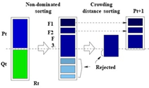
The NDS [6] method, is a commonly utilized technique for solving multi-objective optimization problems. It involves selecting non-dominated individuals within the population and creating a hierarchical structure, representing a set of optimal solutions. The method sorts the population into several non-dominated layers, allowing for the identification of high-quality solutions that are diverse and well-spread across the pareto front. The algorithm assigns rank to individuals, which are determined by their degree of non-domination. The individuals that are best and not dominated by any other solution are given the first rank. This mechanism is repeated until the complete population has been sorted, and individuals are assigned ranks based on their level of domination. NDS is an effective method for finding a set of high-quality solutions that are well-spread across the pareto front. The principle of NDS is demonstrated in Figure 1.
Figure 1. Principle of Non-dominated sorting method [6]
2.3 Bi-Goal Evolution (BIGE)
Li et al. [30] proposed an innovative mechanism called Bi-Goal Evolution (BIGE). This mechanism is designed to formulate a selection strategy that is well-suited for extensive objective spaces. This approach converts a high-dimensional objective space into a bi-objective space, effectively considering the proximity and crowding degree of solutions within the population. The proximity calculation (Eprox) for a given individual s is computed by aggregating its individual objective values into a single comprehensive objective value, as shown in the Eq. (5):
$E_{\mathrm{Pr} o x}=\sum_{i=1}^k E^i(s)$ (5)
Here, “k” represents the total count of objectives, and Ei(s) refers to the goal value of the individual "s" in the ith goal.
Calculating the crowding degree (ECrow) of an solution (s1) within the pareto front set (F) involves the following estimation:
$E_{\text {Crow }}(s 1)=\left(\sum_{s 2 \in F ; s 2 \neq s 1} \operatorname{shar}(s 1, s 2)\right)^{1 / 2}$ (6)
where, shar(s1, s2) means sharing function between two individuals s1 and s2, which is elucidated in Eq. (7):
$\begin{aligned} & \operatorname{shar}\left(s_1, s_2\right)=\left\{\begin{array}{l}\left(0.5\left(1-\frac{\operatorname{Edist}\left(s_1, s_2\right)}{r}\right)\right)^2, \text { if } \operatorname{Edist}\left(s_1, s_2\right)<r, \\ E_{\operatorname{Pr} o x}\left(s_1\right)<E_{\operatorname{Pr} o x}\left(s_2\right) \\ \left(1.5\left(1-\frac{\operatorname{Edist}\left(s_1, s_2\right)}{r}\right)\right)^2, \text { if } \operatorname{Edist}\left(s_1, s_2\right)<r, \\ E_{\operatorname{Pr} o x}\left(s_1\right)>E_{\operatorname{Pr} o x}\left(s_2\right) \\ \text { rand }\left(), \text { if Edist }\left(s_1, s_2\right)<r, E_{\operatorname{Pr} o x}\left(s_1\right)=E_{\operatorname{Pr} o x}\left(s_2\right)\right. \\ 0, \text { otherwise }\end{array}\right.\end{aligned}$ (7)
In this context, Edist(s1, s2) is the euclidean distance between two solutions (s1, s2). The parameter "r" signifies the niche radius, computed using "N" and "K" which respectively denote the population size and the total count of objectives.
$r=\frac{1}{\sqrt[k]{N}}$ (8)
Figure 2. The principle of BIGE strategy [30]
More importantly, in this mechanism of BIGE, using the sharing function mentioned above permits neighbouring solutions to be placed at a distance. And then, the new parameters (EProx) and (ECrow) are estimated using Eq. (5) and Eq. (6), respectively. The principle of BIGE is depicted in Figure 2.
2.4 Harris Hawks Optimization (HHO)
HHO [26] is a newly introduced Algorithm that emulates the Harris hawk chasing behaviour. Below, the mathematical model of this method is presented.
2.4.1 Exploration phase
During this stage, the Hawks are diffused in random areas and use two alternative strategies to find prey:
$\begin{aligned} & L(i t+1)=\left\{\begin{array}{l}L_{\text {rand }}(i t)-r_1\left|L_{\text {rand }}(i t)-2 r_2 L(i t)\right|, q \geq 0.5 \\ \left(L_{\mathrm{Pr} e \mathrm{y}}(i t)-L_{A v}(i t)\right)-r_3\left(T+r_4(F-T)\right), q<0.5\end{array}\right.\end{aligned}$ (9)
where, L(it+1) denotes the Location of Hawks for the subsequent repetition, L(it) is the actual location of hawks, LPrey(it) is the actual location of the prey. r1, r2, r3, r4, and q are assigned randomly in (0, 1). F and T represent the upper and lower limits of positions, respectively, Lrand signifies an individual hawk selected at random from the population, and LAv represents the mean locations of the individuals which is determined by:
$L_{A v}(i t)=\frac{1}{N} \sum_{i t=1}^N L_j(i t)$ (10)
In this equation, N, Lj denote the total count of hawk individuals within the population, and the location of each hawk, respectively.
2.4.2 Transition phase
The HHO can exchange diversification and intensification stages in response to the fleeing energy of the rabbit (E), which is computed by:
$E=2 * E_0\left(1-\frac{i t}{i T}\right)$ (11)
where, E0 refers to the rabbit’s energy at the starting point, which is choosing randomly from an interval of -1 to 1. If the value of E exceeds 1, the HHO prioritizes the diversification strategy. Conversely, if E is less than or equal to 1, the intensification strategy is favored. iT is the maximum count of iterations.
2.4.3 Exploitation phase
Based on the prey’s fleeing energy (E) and their chance fleeing probability (r), the hawks employ four distinct pursuit ways. and switch between them as detailed below:
• Soft Besiege strategy {|E|≥0.5, and r≥0.5}
Hawks encircle the prey gently, causing it to become exhausted before launching a sudden attack, which is described as:
$L(i t+1)=\left(L_{\mathrm{Pr} e y}(i t)-L(i t)\right)-E \mid F^* L_{\mathrm{Pr} e y}(i t)-L(i t)$ (12)
The magnitude of the rabbit’s random jumps during the escape process can be expressed by F=(1-r5)∗2, where r5 represents a randomly generated value within the range of 0 to 1.
• Hard Besiege strategy {|E|<0.5, and r≥0.5}
When the rabbit reaches a state of exhaustion and lacks the energy to flee, it may become vulnerable to surprise attacks by hawks without needing them to encircle its intended target. This scenario is described as follows:
$L(i t+1)=L_{\mathrm{Pr} e y}(i t)-E \mid\left(L_{\mathrm{Pr} e y}(i t)-L(i t)\right)$ (13)
• Soft besiege with progressive rapid dives {|E|≥0.5, and r<0.5}
If the rabbit possesses sufficient energy to successfully flee, Hawks may employ a gentle encirclement strategy prior to launching a surprise attack. In such cases, the algorithm calculates the subsequent movement of the Hawks using the equation below:
$Y=L_{\mathrm{Pr} e y}(i t)-E\left|L_{\mathrm{Pr} e y}(i t)^* F-L(i t)\right|$ (14)
We presume that they will descend into a space of D dimensions, guided by the function of levy flight (LF) [32, 33], by adhering to the following formula:
$Z=Y+L F(D) * S$ (15)
We note that D pertains to the dimensions involved in the optimization issue, while S represents a randomly sized vector of 1*D. Furthermore, the calculation of the LF will be computed as follows:
$L F(l)=0.01 * \frac{u^* \sigma}{|v|^{(1 / \beta)}}$ (16)
u and v are selected at random from [0, 1], the value of β remains constant at 1.5, and σ is defined as below:
$\sigma=\left(\frac{\sin (\pi \beta / 2) * \Gamma(1+\beta)}{2^{\frac{(\beta-1)}{2} *} \beta^* \Gamma((1+\beta) / 2)}\right)^{\frac{1}{\beta}}$ (17)
Thus, the calculation model utilized for updating the Hawks’ positions is specified as follows:
$L(i t+1)= \begin{cases}\gamma, & \text { if } F(\gamma)<F(L(i t)) \\ \lambda, & \text { if } F(\lambda)<F(L(i t))\end{cases}$ (18)
• Hard besiege with progressive rapid dives {|E|<0.5, and r<0.5}
Hawks aim to minimize the gap between their mean locations and the fleeing rabbit. This which can be described as follows:
$L($ it +1$)= \begin{cases}\gamma, & \text { if } F\left(\gamma^{\prime}\right)<F(L(i t)) \\ \lambda, & \text { if } F\left(\lambda^{\prime}\right)<F(L(\text { it }))\end{cases}$ (19)
where,
$Y^{\prime}=L_{\mathrm{Pr} e y}(i t)-E\left|F^* L_{\mathrm{Pr} e y}(i t)-L_{A v}(i t)\right|$ (20)
$Z^{\prime}=Y^{\prime}+S^* L F(D)$ (21)
LAv has been defined in Eq. (10).
This section describes the contribution and main features proposed for the GMOHHO algorithm to solve the MOPs.
3.1 The initialization phase
Firstly, GMOHHO generates the initial population (P) of N Hawks within the defined search space, with each Hawk representing a potential solution to the MOP. Then, according to the M objectives, evaluating each solution from this population is necessary. Moreover, the archive (Ar) is initialized by selecting the non-dominated solutions from the initial population (P). From this archive, the leader solutions (the best solutions) are chosen as guides to direct the main population towards convergence with the true pareto front.
3.2 The offspring phase
Following the initialization step, the GMOHHO employs the exploration and exploitation strategies to investigate the MOP’s search space and prevent being trapped in a situation of stagnancy. Throughout iterations (it), each Harris Hawk upgrades its location using the initial energy (E0), the escaping energy (E), the parameter (q), and the rabbit’s fleeing chance (r) in the range [0,1]. When the energy level E is greater than 1 in GMOHHO, the location of each Hawak Liis updated using 02 exploration strategies that depend on a random number q. If q is less than 0.5, then the hawk Liupdates its position based on the prey solution, the mean location of the actual Hawks population, and a location prodecuced at random. Alternatively, the location of Hawk Liis updated by considering the location of a randomly chosen Hawk from the actual population P(it). This switching between the two exploration strategies allows the Hawk population to search the most potential regions of the search area. Conversely, when E is less than 1, GMOHHO focuses primarily on exploitation strategies to optimize the search process. It employs a decision-making mechanism based on the fleeing chance parameter (r) to determine the appropriate exploitation strategy for exploring the search space of the MOP, thereby improving its effectiveness in finding best solutions.
As stated before, The GMOHHO algorithm employs the four exploitation strategies utilized in the standard HHO method but with an added layer of guidance provided by using multi-leaders solutions (rabbits) selected from the archive population. In contrast to the HHO method, which selects only one leader rabbit from the current population, the GMOHHO method benefits from a more diverse set of guidance to improve its performance. After updating step, the resulting positions are stored in the offspring population (Op). This population consists of N solutions and is considered a temporary population created from the actual population. After that, the GMOHHO updates the archive population by selecting the optimal solutions from the combined population of 2N individuals, comprising both the existing population (P) and the newly generated offspring population (Op). Therefore, a selection procedure (2) based on the Bi-Goal Evolution and NDS is employed on the collective population. This is done to reduce the population size effectively and identify only the N most optimal solutions for the upcoming generation. The subsequent subsection will provide a comprehensive description of the environmental selection strategy.
3.3 The size adjustment phase
The selection procedure is of paramount importance in ensuring the effectiveness of any evolutionary algorithm. In the case of our study, as previously mentioned, three strategies are utilized for selection purposes. Firstly, NDS is utilized to promote the convergence of solutions. Secondly, the Bi-Goal optimization technique is utilized to attain a harmonious equilibrium between convergence and diversity. Finally, random selection is used to ensure good diversity of solutions.
These strategies are elaborated upon in detail through three main steps, as outlined below, and visualized in a flowchart (Figure 3).
3.3.1 The first step
In this step, a temporary merged population $C($ it $)=P($ it $)$ $\cup O p($ it $)$ is created. As expected, the population size of $\mathrm{C}$ is $2 \mathrm{~N}$ (Overflowing problem). Thereby, this merged set is divided into many layers (F1, F2, ...Fn). These layers are determined using Non-Dominated Sorting method, which categorizes individuals based on their level of dominance and assigns them to different layers accordingly. Next, the population for the subsequent generation, P(it+1), is formed by selecting individuals from the first layer F1, F2, and so on until the population size reaches or surpasses N. The solutions in the first layer (F1) are the most promising solutions, while those in the subsequent layers (F2, F3,.. etc.) are progressively less promising. Only the individuals from the most promising layers are added to the population for the next generation, ensuring the preservation and evolutionary refinement of the optimal solutions over time. In the event that the size of layer F1 falls below the target size of N, the remaining individuals needed to fulfill the population quota of N are selected from successive layers in order of their ranking. Specifically, individuals from layer F2 are chosen during the second round, followed by individuals from layer F3 and so forth. This process continues until the critical layer Fi is reached, which is defined as the layer at which $\left|F_1 \cup F_2 \cup \ldots . F_{i-1}\right| \leq N$ and $\mid F_1$ $\cup F_2 \cup \ldots F_i \mid>N$. The addition of individuals to the population is then halted.
3.3.2 The second step
We employ the Bi-Goal optimization strategy for each member of the last accepted Fiset (Critical layer) to estimate the two new objectives, proximity(EProx) and the Crowding degree(ECrow). To pick exactly N solutions, the individuals of layer Fi are partitioned into many layers (Fi1, Fi2..., Fik) according to non-dominance relation based on the two new goals EProxand ECrow. And then, to fill the population P(it + 1), we add (N-|P(it+1)|) solutions from successive layers (Fi1, Fi2,..., Fik) in order of their rating till the critical layer (Fik) will be identified, where $\left|F_{i 1} \cup F_{i 2} \cup \ldots F_{i k-1}\right| \leq N$ and $\mid F_{i 1} \cup F_{i 2} \cup \ldots F_{i k}$ $\mid>N$.
3.3.3 The third step
Finally, the remaining solutions (N- | P(it + 1) |) required to replenish the population P(it + 1) will be loaded randomly from the last accepted layer (Fin) set. Ultimately, these processes are iteratively executed until reaching the maximum allowed iteration, with the archive individuals being the optimal solutions obtained by the MOHHO algorithm.
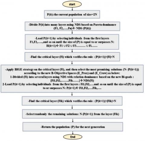
The three aforementioned phases are effectively demonstrated in the accompanying flowchart (refer to Figure 4).
Figure 3. Flowchart of selection procedure
Figure 4. Flowchart of GMOHHO algorithm
This part evaluates the efficacy of the GMOHHO method in handling various MOPs. Firstly, an overview of the experimental setup is provided. Subsequently, the benchmark functions used and the parameters applied to the comparative methods in this study are described. Finally, the statistical findings of the evaluated algorithms are presented and analyzed.
4.1 Experimental setup
We evaluated and compared the GMOHHO algorithm with well-known algorithms from various perspectives using two performance indicators: the Inverted Generational Distance (IGD) [34] and the Hyper Volume (HV) [35]. GMOHHO were implemented using the MATLAB (R2016a) programming language on a 64-bit Windows 10 operating system. The experimental trials were executed using a computer that featured an Intel Core(TM) i5-7300HQ CPU and 8GB of RAM. To ensure reliable results and mitigate the impact of randomness, we performed 31 runs of each comparative method, with each run consisting of 1000 iterations. All test cases were conducted with a population size of 100.
4.2 Test functions and compared algorithms
Table 1. Attributes of test functions
|
Test Function |
Characteristics |
|
ZDT1 |
Convex pareto front. |
|
ZDT2 |
Non-Convex pareto front |
|
ZDT3 |
Discontinuous front |
|
ZDT4 |
221 local optimal pareto fronts (multi-Modal) |
|
ZDT6 |
Non-uniform search space |
|
DTLZ1 |
Linear pareto front |
|
DTLZ2 |
Spherical pareto front |
|
DTLZ3 |
Many pareto front |
|
DTLZ4 |
Pareto front with a dense set of points near fM-f1 |
|
DTLZ5 |
The ability to converge to a degenerated curve |
|
DTLZ6 |
It involves 2M − 1 discontinuous pareto front |
|
DTLZ7 |
Pareto front: mix of a hyperplane and a straight line |
|
MaF1 |
Linear, no one optimum in any set of objectives |
|
MaF2 |
Concave, no one optimum in any set of objectives |
|
MaF3 |
Convex, multimodal curve |
|
MaF4 |
Concave, multimodal, weak scalability, and no a unique optimum within any set of objectives |
|
MaF5 |
Convex, asymmetric, and exhibiting poor scaling |
|
MaF6 |
Concave, degenerate curve |
|
MaF7 |
Mixed, disconnected, multimodal |
Table 2. Parameters of algorithms
|
Algorithm |
Parameters |
|
MSSA |
The coefficient $a 1=e^{-\left(\frac{4 k}{K}\right)}, a 2$ and $a 3$ : random numbers inside [0,1] |
|
MOEA/D |
Subproblems: M=100, mutation rates: cr=0,5, numbers of neighbors: u=10, the index of dispersion η=30, probability of selection δ=30 |
|
MOGWO |
Grid Inflation σ=0,1, Grids number NG=10, Selection pressure γ=2, and β=4 |
|
GMOHHO |
Scalling coefficients $r_1, r_2, r_3, r_4, u, v$ and Fleeing chance q, are random numbers inside [0,1], Initial prey energy $E_0=2$ rand ()$-1$, Jump strengh $J=2(1-$ rand ()) |
To evaluate the efficacy of the newly introduced GMOHHO algorithm, an extensive collection of benchmark functions was utilized for evaluation. These benchmarks were carefully selected from well-established categories, namely the ZDT-series [36] (consisting of five bi-objective functions), the DTLZ series [37] (consisting of a set of seven three-objective functions), and the MaF series [38] (encompassing seven many-objective functions). The attributes of these evaluation functions are outlined in Table 1.
For the purpose of conducting a comparative study, three reputable benchmarking techniques, namely MSSA [19], MOEAD [11], and MOGWO [14], were chosen. The initial parameters of each algorithm, as recommended in their original sources, are provided in Table 2. All test methods were conducted with a population volume of 100. to reduce the impact of randomness, we conducted 31 runs of each comparative method, each consisting of 1000 iterations.
4.3 Comparative experimental results on ZDT serie
In this section, we comprehensively evaluate the efficacy of the suggested GMOHHO algorithm specifically in the context of bi-objective problems represented by the ZDT series. To effectively assess its performance, we conduct a comparative analysis between the GMOHHO and other well-established multi-objective methods. The results obtained from this comparative analysis are presented in Tables 3 and 4, where we utilize the IGD and HV indicators, respectively, to measure the performance of the algorithm.
Table 3, which displays the IGD indicator, reveals that the GMOHHO algorithm consistently outperformed all other tested techniques across the entire range of ZDT benchmark problems. This outcome clearly signifies the superior performance of the GMOHHO algorithm in addressing the specific challenges posed by these problems. Similarly, Table 4, which presents the HV measure, consistently showcases the GMOHHO algorithm's superiority over the other methods across all test functions. The statistically acquired results not only validate the efficacy of the GMOHHO algorithm but also highlight its capability to effectively handle MOPs. However, to provide a more comprehensive analysis, it is crucial to delve into the reasons behind the observed performance differences among the algorithms and elucidate how the proposed GMOHHO method addresses any shortcomings of the other methods.
One potential reason for the GMOHHO algorithm's superior performance could be attributed to its innovative incorporation of hybridization between three strategies: the Bi-Goal Evolution (BIGE), Non-Dominated Sorting (NDS), and Multi-Leader Selection (MLS). This hybridization allows the GMOHHO algorithm to effectively balance exploration and exploitation, leading to improved convergence and search capabilities. In contrast, the comparative algorithms may exhibit limitations in terms of their exploration and exploitation capabilities, as well as their adaptability to diverse problem domains. These limitations can lead to suboptimal solutions and hinder their performance when faced with the complexities of MOPs.
It's essential to acknowledge that while the GMOHHO method demonstrated significant advantages, there are still potential areas for improvement. For instance, further investigations could be conducted to optimize the algorithm's parameter settings to enhance its overall performance. Additionally, the algorithm's robustness and scalability could be explored and validated on larger-scale MOPs to ensure its applicability to real-world problem domains.
Table 3. Results of IGD metric on ZDT test functions
|
|
Algorithms |
Best |
Worst |
Mean |
|
ZDT1 |
GMOHHO |
4,77E-4b |
1,68E-03 |
6,60E-04 |
|
MOGWO |
5,89E-04 |
6,10E-03 |
1,50E-03 |
|
|
MOEAD |
5,41E-04 |
3,14E-03 |
1,15E-03 |
|
|
MSSA |
3,15E-03 |
7,20E-03 |
4,73E-03 |
|
|
ZDT2 |
GMOHHO |
4,50E-04 |
5,66E-03 |
1,29E-03 |
|
MOGWO |
7,93E-04 |
2,31E-02 |
6,45E-03 |
|
|
MOEAD |
3,99E-04 |
6,24E-02 |
2,20E-02 |
|
|
MSSA |
3,65E-03 |
1,16E-02 |
5,30E-03 |
|
|
ZDT3 |
GMOHHO |
5,07E-04 |
1,37E-03 |
7,21E-04 |
|
MOGWO |
3,06E-04 |
3,26E-03 |
9,66E-04 |
|
|
MOEAD |
6,03E-03 |
2,39E-02 |
1,04E-02 |
|
|
MSSA |
4,50E-03 |
1,16E-02 |
7,18E-03 |
|
|
ZDT4 |
GMOHHO |
4,35E-04 |
9,13E-04 |
6,20E-04 |
|
MOGWO |
2,89E-02 |
7,19E-01 |
2,88E-01 |
|
|
MOEAD |
2,03E-01 |
2,56E+00 |
1,16E+00 |
|
|
MSSA |
6,93E-02 |
5,01E-01 |
1,94E-01 |
|
|
ZDT6 |
GMOHHO |
2,91E-04 |
1,14E-03 |
4,79E-04 |
|
MOGWO |
2,88E-04 |
2,99E-03 |
1,45E-03 |
|
|
MOEAD |
3,52E-04 |
1,69E-01 |
3,35E-02 |
|
|
MSSA |
6,68E-04 |
4,21E-03 |
2,05E-03 |
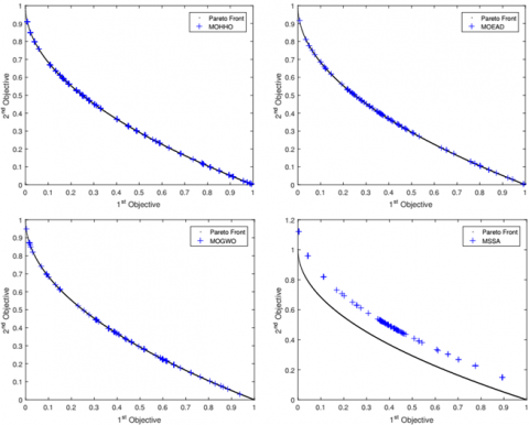
The extensive evaluation of the GMOHHO in comparison to established methods on the ZDT benchmark series, as supported by both statistical metrics and visual convergence curves (Figures 5-7), confirms its superior performance in generating well-spread non-dominated solutions along the optimal pareto front.
Table 4. Results of HV metric on ZDT test functions
|
|
Algorithms |
Best |
Worst |
Mean |
|
ZDT1 |
GMOHHO |
7,11E-01 |
6,97E-01 |
7,07E-01 |
|
MOGWO |
7,09E-01 |
6,48E-01 |
6,93E-01 |
|
|
MOEAD |
7,11E-01 |
5,90E-01 |
6,85E-01 |
|
|
MSSA |
5,96E-01 |
4,83E-01 |
5,48E-01 |
|
|
ZDT2 |
GMOHHO |
4,39E-01 |
3,95E-01 |
4,33E-01 |
|
MOGWO |
4,23E-01 |
9,09E-02 |
3,39E-01 |
|
|
MOEAD |
4,38E-01 |
0,00E+00 |
7,52E-02 |
|
|
MSSA |
3,13E-01 |
1,91E-01 |
2,61E-01 |
|
|
ZDT3 |
GMOHHO |
5,91E-01 |
5,76E-01 |
5,81E-01 |
|
MOGWO |
6,00E-01 |
5,48E-01 |
5,81E-01 |
|
|
MOEAD |
5,80E-01 |
1,30E-01 |
4,22E-01 |
|
|
MSSA |
6,46E-01 |
4,70E-01 |
5,55E-01 |
|
|
ZDT4 |
GMOHHO |
7,12E-01 |
7,02E-01 |
7,08E-01 |
|
MOGWO |
9,09E-02 |
0,00E+00 |
5,86E-03 |
|
|
MOEAD |
0,00E+00 |
0,00E+00 |
0,00E+00 |
|
|
MSSA |
0,00E+00 |
0,00E+00 |
0,00E+00 |
|
|
ZDT6 |
GMOHHO |
3,84E-01 |
7,99E-02 |
3,21E-01 |
|
MOGWO |
3,85E-01 |
3,26E-01 |
3,59E-01 |
|
|
MOEAD |
3,83E-01 |
0,00E+00 |
2,08E-01 |
|
|
MSSA |
3,76E-01 |
2,52E-01 |
3,38E-01 |
Figure 5. Best pareto fronts generated by each algorithm on ZDT1
Figure 6. Best pareto fronts generated by each method on ZDT2
Figure 7. Best pareto fronts generated by each method on ZDT4
4.4 Comparative experimental results on DTLZ serie
Table 5. Results of IGD metric on DTLZ test functions
|
|
Algorithms |
Best |
Worst |
Mean |
|
DTLZ1 |
GMOHHO |
6,80E-04 |
2,72E-02 |
4,07E-03 |
|
MOGWO |
3,49E-02 |
2,01E-01 |
1,25E-01 |
|
|
MOEAD |
3,71E-02 |
2,68E-01 |
1,58E-01 |
|
|
MSSA |
6,01E-03 |
2,70E-01 |
6,39E-02 |
|
|
DTLZ2 |
GMOHHO |
1,37E-03 |
4,00E-03 |
1,86E-03 |
|
MOGWO |
6,69E-03 |
1,03E-02 |
7,88E-03 |
|
|
MOEAD |
1,32E-03 |
1,82E-03 |
1,58E-03 |
|
|
MSSA |
5,28E-03 |
8,21E-03 |
7,32E-03 |
|
|
DTLZ3 |
GMOHHO |
1,74E-03 |
1,49E-02 |
8,87E-03 |
|
MOGWO |
1,70E+00 |
2,97E+00 |
2,78E+00 |
|
|
MOEAD |
4,08E-01 |
1,71E+00 |
1,16E+00 |
|
|
MSSA |
1,01E-01 |
2,37E+00 |
1,56E+00 |
|
|
DTLZ4 |
GMOHHO |
1,48E-03 |
1,39E-02 |
3,55E-03 |
|
MOGWO |
1,76E-03 |
2,80E-03 |
2,20E-03 |
|
|
MOEAD |
1,36E-03 |
1,43E-02 |
5,52E-03 |
|
|
MSSA |
4,57E-03 |
1,02E-02 |
6,80E-03 |
|
|
DTLZ5 |
GMOHHO |
2,42E-04 |
1,06E-03 |
3,82E-04 |
|
MOGWO |
8,71E-04 |
2,40E-03 |
1,50E-03 |
|
|
MOEAD |
2,01E-04 |
7,83E-04 |
4,41E-04 |
|
|
MSSA |
6,53E-04 |
3,72E-03 |
1,55E-03 |
|
|
DTLZ6 |
GMOHHO |
5,74E-04 |
1,93E-02 |
6,79E-03 |
|
MOGWO |
7,58E-04 |
7,31E-03 |
2,19E-03 |
|
|
MOEAD |
2,49E-04 |
1,09E-03 |
5,43E-04 |
|
|
MSSA |
6,17E-04 |
5,75E-03 |
1,84E-03 |
|
|
DTLZ7 |
GMOHHO |
1,09E-03 |
6,42E-03 |
1,94E-03 |
|
MOGWO |
2,71E-03 |
9,95E-03 |
5,58E-03 |
|
|
MOEAD |
2,69E-03 |
6,52E-02 |
2,42E-02 |
|
|
MSSA |
6,72E-03 |
2,52E-02 |
1,12E-02 |
Note: Best results are marked in bold
Tables 5-6 present the comprehensive statistical findings of the evaluated methods on the three-objective test problems from the DTLZ series, focusing on diversification evaluation criteria, convergence, and variety. The experimental findings demonstrate the superior performance of the proposed GMOHHO compared to other methods. This is evident in its enhanced convergence rate and its ability to generate a more diverse set of optimal solutions.
Table 6. Results of HV metric on DTLZ test functions
|
|
Algorithms |
Best |
Worst |
Mean |
|
DTLZ1 |
GMOHHO |
7,74E-01 |
5,61E-01 |
7,09E-01 |
|
MOGWO |
0,00E+00 |
0,00E+00 |
0,00E+00 |
|
|
MOEAD |
0,00E+00 |
0,00E+00 |
0,00E+00 |
|
|
MSSA |
1,36E-02 |
0,00E+00 |
4,37E-04 |
|
|
DTLZ2 |
GMOHHO |
5,34E-01 |
3,11E-01 |
5,01E-01 |
|
MOGWO |
3,09E-01 |
1,15E-01 |
4,48E-01 |
|
|
MOEAD |
4,04E-01 |
1,30E-01 |
4,79E-01 |
|
|
MSSA |
3,64E-02 |
1,33E-02 |
1,31E-02 |
|
|
DTLZ3 |
GMOHHO |
5,24E-01 |
2,37E-01 |
4,16E-01 |
|
MOGWO |
0,00E+00 |
0,00E+00 |
0,00E+00 |
|
|
MOEAD |
0,00E+00 |
0,00E+00 |
0,00E+00 |
|
|
MSSA |
0,00E+00 |
0,00E+00 |
0,00E+00 |
|
|
DTLZ4 |
GMOHHO |
5,36E-01 |
9,09E-02 |
3,87E-01 |
|
MOGWO |
4,50E-01 |
3,65E-01 |
4,18E-01 |
|
|
MOEAD |
5,00E-01 |
3,72E-02 |
3,85E-01 |
|
|
MSSA |
1,20E-02 |
1,95E-02 |
1,14E-01 |
|
|
DTLZ5 |
GMOHHO |
1,96E-01 |
1,88E-01 |
1,92E-01 |
|
MOGWO |
1,55E-01 |
1,26E-01 |
1,73E-01 |
|
|
MOEAD |
1,85E-01 |
1,50E-01 |
1,90E-01 |
|
|
MSSA |
6,13E-03 |
1,38E-02 |
4,70E-03 |
|
|
DTLZ6 |
GMOHHO |
1,78E-01 |
0,00E+00 |
1,50E-01 |
|
MOGWO |
1,32E-01 |
1,51E-02 |
1,82E-01 |
|
|
MOEAD |
1,95E-01 |
1,82E-01 |
1,92E-01 |
|
|
MSSA |
1,47E-02 |
3,82E-02 |
2,64E-03 |
|
|
DTLZ7 |
GMOHHO |
2,24E-01 |
1,34E-01 |
1,62E-01 |
|
MOGWO |
2,08E-01 |
3,34E-02 |
9,56E-02 |
|
|
MOEAD |
1,42E-01 |
0,00E+00 |
1,33E-02 |
|
|
MSSA |
1,40E-01 |
0,00E+00 |
5,36E-02 |
Note: Best results are marked in bold
Figure 8. Best pareto fronts generated by each method on DTLZ2
Table 5 summarizes the obtained findings of the IGD measure for the DTLZ series used in our study. The findings demonstrate that the GMOHHO method consistently achieves superior heterogeneity of non-dominated solutions compared to other well-known methods, as indicated by the lower IGD values. However, for the DTLZ2 and DTLZ6 test functions, the MOEAD method achieved slightly better results than our algorithm, ranking it second in these cases. Furthermore, Table 6 provides the findings obtained from the HV measure for the aforementioned benchmark tests. Our statistical analysis reveals that the optimal solutions generated by the GMOHHO outperform those of other well-known methods, particularly for DTLZ1, DTLZ2, DTLZ3, DTLZ5, and DTLZ7, as indicated by higher HV findings. However, it is noteworthy to mention that the MOGWO and MOEAD algorithms achieved better average HV values for DTLZ4 and DTLZ6, respectively.
Furthermore, we analyzed the convergence behavior of the the DTLZ series’ comparison algorithms and plotted the corresponding convergence curves, as shown in Figures 8-9. Our observations indicate that the optimal solutions obtained by the GMOHHO algorithm are well-distributed for the real pareto front for all the tested problems. Specifically, the suggested algorithm exhibited exemplary convergence behavior and achieved diverse Pareto solutions for all the DTLZ test problems. The algorithm's dynamic hybrid approach enables it to outperform other methods in most cases. However, certain areas for improvement have been identified, particularly regarding the performance on specific test functions. Future research can focus on addressing these limitations.
4.5 Comparative experimental results MaF on series
Table 7. Results of IGD metric on MaF test functions
|
|
Algorithms |
Best |
Worst |
Mean |
|
MaF1 |
GMOHHO |
8,51E-03 |
2,06E-02 |
1,20E-02 |
|
MOGWO |
5,05E-02 |
7,54E-02 |
6,42E-02 |
|
|
MOEAD |
8,88E-03 |
1,34E-02 |
1,06E-02 |
|
|
MSSA |
3,32E-02 |
5,62E-02 |
4,52E-02 |
|
|
MaF2 |
GMOHHO |
1,31E-02 |
1,79E-02 |
1,52E-02 |
|
MOGWO |
7,59E-02 |
9,96E-02 |
8,87E-02 |
|
|
MOEAD |
1,34E-02 |
2,43E-02 |
1,69E-02 |
|
|
MSSA |
3,32E-02 |
5,62E-02 |
4,52E-02 |
|
|
MaF3 |
GMOHHO |
1,11E-02 |
1,04E-01 |
5,32E-02 |
|
MOGWO |
3,23E+03 |
8,00E+03 |
5,86E+03 |
|
|
MOEAD |
1,15E+03 |
3,37E+04 |
9,82E+03 |
|
|
MSSA |
1,86E+02 |
4,75E+03 |
2,96E+03 |
|
|
MaF4 |
GMOHHO |
2,46E-01 |
5,47E-01 |
3,90E-01 |
|
MOGWO |
3,00E-01 |
1,10E+02 |
7,67E+01 |
|
|
MOEAD |
1,92E+01 |
6,65E+01 |
3,54E+01 |
|
|
MSSA |
8,34E+00 |
7,94E+01 |
5,39E+01 |
|
|
MaF5 |
GMOHHO |
3,95E-02 |
2,61E-01 |
6,53E-02 |
|
MOGWO |
5,90E-02 |
9,66E-02 |
7,60E-02 |
|
|
MOEAD |
5,60E-02 |
2,59E-01 |
1,22E-01 |
|
|
MSSA |
1,25E-01 |
3,58E-01 |
2,47E-01 |
|
|
MaF6 |
GMOHHO |
1,62E-03 |
3,20E-03 |
2,24E-03 |
|
MOGWO |
3,23E-03 |
8,18E-02 |
3,80E-02 |
|
|
MOEAD |
1,45E-03 |
9,78E-03 |
4,22E-03 |
|
|
MSSA |
5,54E-03 |
2,52E-02 |
1,47E-02 |
|
|
MaF7 |
GMOHHO |
1,07E-02 |
6,54E-02 |
1,97E-02 |
|
MOGWO |
2,40E-02 |
9,18E-02 |
5,28E-02 |
|
|
MOEAD |
5,56E-02 |
4,77E-01 |
1,96E-01 |
|
|
MSSA |
6,61E-02 |
2,66E-01 |
9,59E-02 |
Note: Best results are marked in bold
The results obtained from the benchmarks functions with many-objective within the MaF series, as presented in Tables 7-8, highlight the exceptional capabilities of the proposed GMOHHO in generating heightened convergence and a diverse set of optimal solutions. According to the IGD metric, the results in Table 7 demonstrate that the GMOHHO method consistently outperforms the competing methods across almost all the MaF series, converging quickly to the real pareto front. The only exception is the MaF1 test problem, where the MOEAD algorithm performed slightly better.
Table 8. Results of HV metric on MaF test functions
|
|
Algorithms |
Best |
Worst |
Mean |
|
MaF1
|
GMOHHO |
1,97E-01 |
1,41E-01 |
1,77E-01 |
|
MOGWO |
7,53E-02 |
3,15E-02 |
4,73E-02 |
|
|
MOEAD |
1,97E-01 |
1,80E-01 |
1,89E-01 |
|
|
MSSA |
1,15E-01 |
4,52E-02 |
7,46E-02 |
|
|
MaF2
|
GMOHHO |
2,05E-01 |
1,96E-01 |
2,02E-01 |
|
MOGWO |
6,93E-02 |
5,57E-02 |
5,90E-02 |
|
|
MOEAD |
1,99E-01 |
1,81E-01 |
1,92E-01 |
|
|
MSSA |
9,38E-02 |
5,10E-02 |
6,53E-02 |
|
|
MaF3
|
GMOHHO |
9,19E-01 |
5,03E-02 |
5,54E-01 |
|
MOGWO |
0,00E+00 |
0,00E+00 |
0,00E+00 |
|
|
MOEAD |
0,00E+00 |
0,00E+00 |
0,00E+00 |
|
|
MSSA |
0,00E+00 |
0,00E+00 |
0,00E+00 |
|
|
MaF4
|
GMOHHO |
2,56E-01 |
1,05E-02 |
1,98E-01 |
|
MOGWO |
1,70E-01 |
0,00E+00 |
5,48E-03 |
|
|
MOEAD |
0,00E+00 |
0,00E+00 |
0,00E+00 |
|
|
MSSA |
0,00E+00 |
0,00E+00 |
0,00E+00 |
|
|
MaF5
|
GMOHHO |
5,36E-01 |
2,96E-01 |
5,01E-01 |
|
MOGWO |
4,47E-01 |
3,89E-01 |
4,22E-01 |
|
|
MOEAD |
4,87E-01 |
3,07E-01 |
4,16E-01 |
|
|
MSSA |
3,78E-01 |
8,75E-02 |
1,89E-01 |
|
|
MaF6
|
GMOHHO |
1,96E-01 |
1,87E-01 |
1,92E-01 |
|
MOGWO |
1,66E-01 |
0,00E+00 |
8,76E-02 |
|
|
MOEAD |
1,96E-01 |
1,38E-01 |
1,87E-01 |
|
|
MSSA |
1,88E-01 |
1,09E-01 |
1,47E-01 |
|
|
MaF7 |
GMOHHO |
2,69E-01 |
1,99E-01 |
2,53E-01 |
|
MOGWO |
2,25E-01 |
3,42E-02 |
1,07E-01 |
|
|
MOEAD |
6,25E-02 |
0,00E+00 |
8,25E-03 |
|
|
MSSA |
1,26E-01 |
0,00E+00 |
6,32E-02 |
Analyzing the findings using the HV metric, as presented in Table 8, reveals that the GMOHHO algorithm surpasses the other methods for the majority of the examined issues, indicating its capacity to produce high-quality of solutions. However, similar to the IGD metric, the MOEAD algorithm exhibits a slight superiority over other algorithms for the MaF1 problem. Overall, these findings conclusively showcase the superior performance of the GMOHHO method in effectively addressing MOPs, surpassing the capabilities of the algorithms under investigation.
To gain deeper insights into the performance differences among the algorithms, let us discuss the underlying reasons. The GMOHHO algorithm employs a dynamic hybrid approach that combines BIGE, the NDS, and Multi-leader selection techniques. This unique combination empowers the algorithm to adeptly navigate the solution space, leading to a wider variety of optimal solutions. The method's efficient convergence to the real pareto front can be attributed to its ability to to harmonize diversification and intensification, thereby optimizing the trade-off between convergence and diversity.
Furthermore, Figures 10-11 provide graphical representations of the convergence behavior of the compared methods for the benchmark issues. The visualizations clearly illustrate that, across all the studied issues, the optimal solutions generated by the GMOHHO method are uniformly distributed and closely align with the ideal pareto front. This further substantiates the algorithm's ability to produce solutions characterized by a superior level of quality.
Despite the success of the GMOHHO method, it is important to acknowledge its limitations and identify areas for improvement. Further investigation could be conducted to understand the reasons behind the MOEAD algorithm's better performance on the MaF1 problem and explore potential modifications to enhance the GMOHHO algorithm's capabilities in solving such challenges. Additionally, future research could focus on evaluating our method on larger-scale and more intricacy multi-objective optimization issues to validate its scalability and robustness.
Figure 9. Best pareto fronts generated by each method on DTLZ7
Figure 10. Best pareto fronts generated by each algorithm on MaF1
Figure 11. Best pareto fronts generated by each method on MaF3
4.6 Running time analysis
The running time was recorded as the total computational time required by each algorithm to complete the optimization process on a given benchmark problem. This includes the time taken for initialization, iterations, and any necessary calculations. In our study, we conducted an evaluation of the algorithms' performance with respect to their running time on each test problem. To measure this, we recorded the time taken to complete an iteration of 1000. The outcomes are presented in Table 9.
Table 9. Execution time comparison of the four algorithms
|
|
Algorithms |
|||
|
Test Functions |
GMOHHO |
MOEA-D |
MOGWO |
MSSA |
|
ZDT1 |
141.8110 |
440.0093 |
668.2665 |
89.9722 |
|
ZDT2 |
136.8550 |
374.8618 |
67.2408 |
55.2313 |
|
ZDT3 |
113.5348 |
371.5014 |
448.3240 |
92.0169 |
|
ZDT4 |
151.5093 |
208.1556 |
76.3337 |
43.3857 |
|
ZDT6 |
160.6806 |
370.6754 |
713.5653 |
49.8646 |
|
DTLZ1 |
104.0166 |
405.8341 |
186.3638 |
56.8196 |
|
DTLZ2 |
121.1297 |
444.8980 |
543.7021 |
222.9273 |
|
DTLZ3 |
101.2963 |
433.9067 |
688.6034 |
78.0878 |
|
DTLZ4 |
112.2558 |
428.1579 |
447.3627 |
150.7616 |
|
DTLZ5 |
114.1447 |
424.8031 |
437.7445 |
153.5962 |
|
DTLZ6 |
113.5271 |
453.2583 |
211.5742 |
28.6178 |
|
DTLZ7 |
124.9172 |
292.8392 |
482.3534 |
83.7363 |
|
MaF1 |
118.9803 |
432.7459 |
751.2107 |
135.9046 |
|
MaF2 |
126.6412 |
441.2643 |
791.1880 |
128.2156 |
|
MaF3 |
102.7200 |
182.9752 |
393.3237 |
45.9072 |
|
MaF4 |
104.6724 |
477.8634 |
252.7810 |
117.4090 |
|
MaF5 |
108.5752 |
647.3135 |
527.3682 |
174.9229 |
|
MaF6 |
108.7966 |
437.5473 |
201.7451 |
66.3366 |
|
MaF7 |
116.7403 |
358.6604 |
683.8026 |
63.2119 |
Note: Best results are marked in bold
Upon analysis, we observed that the MSSA algorithm achieved the best overall results, ranking first for 12 test benchmarks. In terms of execution time, our proposed GMOHHO algorithm demonstrated the fastest performance for the DTLZ3, DTLZ4, DTLZ5, MaF3, MaF6, and MaF7 test problems. Our algorithm also achieved a second-place ranking for the remaining test functions, closely following the MSSA algorithm. There were a few exceptions, specifically for the ZDT2 and ZDT4 problems, where the GMOHHO algorithm ranked third behind the MOGWO method.
It is important to discuss the trade-offs between running time and efficiency indicators, such as IGD and HV. Although the GMOHHO algorithm might not consistently achieve the fastest execution time, it's essential to take into account the algorithm's overall effectiveness. When considering the quality of optimal solutions generated by the algorithms, as evaluated by IGD and HV metrics, the GMOHHO algorithm showcased competitive performance. It consistently outperformed the MOEAD and MOGWO algorithms. It is clear that there is a balance to be struck. Some algorithms may prioritize faster execution times at the expense of solution quality, while others may require more computational resources to attain improved performance. Regarding the GMOHHO, it strikes a favorable balance between running time and performance, achieving reasonable execution times while still generating high-quality non-dominated solutions.
4.7 Wilcoxon statistical test analysis
In this study, we incorporated the non-parametric Wilcoxon test [39] to assess the presence of significant statistical distinctions between the suggested GMOHHO algorithm and the other scrutinized algorithms being compared. The Wilcoxon test was chosen as a suitable statistical tool due to its ability to analyze paired data and handle non-normal distributions.
If the calculated pvalue is equal to or greater than the chosen significance level (α), the outcome would entail the non-rejection of the null hypothesis (H0), indicating that there are no significant improvements associated with the comparative methods. However, if the pvalueis fewer than (α), we deny (H0) to the benefit of the alternative hypothesis (H1), which suggests that there are significant improvements associated with the comparative methods. In our analysis, we used a significance threshold of 5%, and compared the outcomes of two algorithms using the IGD and HV metrics. Specifically, µ1 and µ2 reflect the outcomes of the first and second algorithms, respectively.
The Wilcoxon analysis conducted on the IGD measure involved formulating the ensuing hypotheses:
To perform the Wilcoxon analysis on the HV measure, we formulated the ensuing hypotheses:
Table 10. Test Wilcoxon results for IGD metric
|
GMOHHO vs |
MOEA-D |
MOGWO |
MSSA |
|
ZDT1 |
2,1319E-03 |
1,4534E-08 |
7,0092E-12 |
|
ZDT2 |
1,1840E-10 |
6,3105E-10 |
7,0092E-12 |
|
ZDT3 |
7,0092E-12 |
5,1991E-03 |
7,0092E-12 |
|
ZDT4 |
7,0092E-12 |
7,0092E-12 |
7,0092E-12 |
|
ZDT6 |
0,023 |
0,658 |
3,0226E-03 |
|
DTLZ1 |
7,0092E-12 |
7,0092E-12 |
7,0092E-12 |
|
DTLZ2 |
0,999 |
5,9367E-10 |
2,1689E-09 |
|
DTLZ3 |
7,0092E-12 |
7,0092E-12 |
7,0092E-12 |
|
DTLZ4 |
0,913 |
0,854 |
3,4349E-03 |
|
DTLZ5 |
3,1548E-03 |
7,0092E-12 |
7,0092E-12 |
|
DTLZ6 |
0,964 |
5,0221E-09 |
2,7501E-08 |
|
DTLZ7 |
1,2985E-09 |
3,4349E-03 |
7,0092E-12 |
|
MaF1 |
8,1993E-01 |
7,0092E-12 |
7,0092E-12 |
|
MaF2 |
1,36E-03 |
7,0092E-12 |
7,0092E-12 |
|
MaF3 |
7,0092E-12 |
7,0051E-12 |
7,0092E-12 |
|
MaF4 |
7,0092E-12 |
1,1840E-10 |
7,0092E-12 |
|
MaF5 |
1,2797E-05 |
1,7447E-04 |
4,2855E-11 |
|
MaF6 |
7,2483E-06 |
7,0092E-12 |
7,0092E-12 |
|
MaF7 |
8,5090E-12 |
2,1689E-09 |
2,1399E-04 |
Note: Best results are marked in bold
The null hypothesis (H0) assumes that the IGD and HV scores of the compared methods are either equal to or worse than those of the proposed GMOHHO. Conversely, the the opposing hypothesis (H1) suggests that the IGD and HV scores of the GMOHHO algorithm are superior to those of the comparative methods.
Tables 10-11 present the outcoms of the Wilcoxon statistical evaluations, confirming that the alternative hypothesis (H1) is accepted for the GMOHHO algorithm based on both the IGD and HV measures. The lower IGD values obtained by the GMOHHO algorithm indicate its superior ability to approach the true pareto front. Additionally, the higher HV values demonstrate its effectiveness in achieving better coverage of the Pareto set in contrast to the other methods, with a significance degree of less than 5%. These findings underscore the GMOHHO algorithm's potential in enhancing Pareto set diversity while converging towards the true Pareto front.
Table 11. Test Wilcoxon results for HV metric
|
GMOHHO vs |
MOEA-D |
MOGWO |
MSSA |
|
ZDT1 |
1,9917E-02 |
1,8294E-09 |
7,0092E-12 |
|
ZDT2 |
6,1610E-11 |
4,0593E-10 |
7,0092E-12 |
|
ZDT3 |
8,2041E-11 |
0,979 |
8,3475E-03 |
|
ZDT4 |
2,5259E-13 |
4,9413E-13 |
2,5259E-13 |
|
ZDT6 |
1,3189E-03 |
0,583 |
1,3555E-03 |
|
DTLZ1 |
2,5259E-13 |
2,5259E-13 |
3,5878E-13 |
|
DTLZ2 |
2,5411E-08 |
7,0092E-12 |
7,0092E-12 |
|
DTLZ3 |
2,5259E-13 |
2,5259E-13 |
2,5259E-13 |
|
DTLZ4 |
9,0102E-03 |
8,3475E-03 |
3,6394E-04 |
|
DTLZ5 |
0,236 |
7,0092E-12 |
1,1365E-11 |
|
DTLZ6 |
1,000 |
7,6197E-05 |
0,968 |
|
DTLZ7 |
7,5742E-12 |
3,1185E-04 |
9,3724E-12 |
|
MaF1 |
9,9657E-01 |
7,0092E-12 |
7,0092E-12 |
|
MaF2 |
1,5152E-11 |
7,0092E-12 |
7,0092E-12 |
|
MaF3 |
2,5259E-13 |
2,5259E-13 |
2,5259E-13 |
|
MaF4 |
2,5259E-13 |
6,1796E-13 |
2,5259E-13 |
|
MaF5 |
1,2368E-08 |
1,4206E-10 |
1,1365E-11 |
|
MaF6 |
3,6890E-02 |
7,0092E-12 |
8,5090E-12 |
|
MaF7 |
6,3596E-12 |
3,5535E-11 |
6,9805E-12 |
Note: Best results are marked in bold
While the Wilcoxon test is a robust and widely used non-parametric test, it is important to acknowledge its limitations and assumptions. One assumption is that the observations within each pair are independent and identically distributed. Violation of this assumption may affect the interpretation of the results. Additionally, the Wilcoxon test assumes that the two samples being compared come from the same population, except for a shift in their distributions. It is essential to consider these limitations when interpreting the outcomes of the Wilcoxon test.
In summary, the non-parametric Wilcoxon test was employed to analyze the statistical significance of variances between the proposed GMOHHO and the comparative methods. Its selection was based on its suitability for paired data analysis and robustness against non-normal distributions.
This paper introduced GMOHHO, a Guided Multi-Objective Harris Hawks Optimizer, to address the limitations of the standard HHO method and tackle complex multi-objective optimization problems. The motivation behind developing GMOHHO was to extend the applicability of HHO to multi-objective problems, providing high-quality solutions within reasonable timeframes. We integrated several strategies, including a population archive, efficient multi-leader selection, and the Bi-Goal Evolution (BIGE) framework with Non-Dominated Sorting technique, to augment the algorithm's performance.
The evaluation of GMOHHO on various benchmark functions showcased its superiority over the typical HHO method and other leading-edge multi-objective optimization methods. The results consistently demonstrated its robustness, efficiency, and ability to deliver a broad range of high-quality non-dominated solutions, thus effectively approximating the complete Pareto optimal front.
The proposed GMOHHO algorithm has significant practical benefits and a broader impact in solving complex MOPs. By synergistically merging the strengths of the HHO method with guided search strategies and incorporating multi-objective techniques, GMOHHO offers advantages such as improved convergence, diversity of solutions, and precise approximation of the pareto front.
In summary, the GMOHHO algorithm presents a promising alternative for tackling MOPs of varying sizes. Its impact extends beyond the academic realm, as it offers practical benefits and solutions for real-world challenges. The algorithm's robustness, efficiency, and adeptness in approximating the complete Pareto optimal front make it a valuable approach in addressing MOPs.
Future directions for research include parameter optimization, hybridization with other optimization techniques, scalability evaluation, and application to constrained optimization problems and real-world domains. These avenues will further advance the field and improve the practicality and applicability of the GMOHHO algorithm.
[1] Anupriya, K., Harini, K., Balaji, K., Sudha, K.G. (2022). Spam mail detection using optimization techniques. Ingénierie des Systèmes d’Information, 27(1): 157-163. https://doi.org/10.18280/isi.270119
[2] Ren, F., Wang, J., Zhu, S., Chen, Y. (2019). Multi-objective optimization of combined cooling, heating and power system integrated with solar and geothermal energies. Energy conversion and management, 197: 111866. https://doi.org/10.1016/j.enconman.2019.111866
[3] Jain, A., Nandan, D., Meduri, P. (2023). Data export and optimization technique in connected vehicle. Ingénierie des Systèmes d’Information, 28(2): 517-525. https://doi.org/10.18280/isi.280229
[4] Sharma, S., Kumar, V. (2022). A comprehensive review on multi-objective optimization techniques: Past, present and future. Archives of Computational Methods in Engineering, 29(7): 5605-5633. http://doi.org/10.1007/s11831-022-09778-9
[5] Vachhani, V.L., Dabhi, V.K., Prajapati, H.B. (2015). Survey of multi objective evolutionary algorithms. In 2015 international conference on circuits, power and computing technologies [ICCPCT-2015], Nagercoil, India, pp. 1-9. http://doi.org/10.1109/ICCPCT.2015.7159422
[6] Deb, K., Pratap, A., Agarwal, S., Meyarivan, T.A.M.T. (2002). A fast and elitist multiobjective genetic algorithm: NSGA-II. IEEE Transactions on Evolutionary Computation, 6(2): 182-197. http://doi.org/10.1109/4235.996017
[7] Srinivas, N., Deb, K. (1994). Muiltiobjective optimization using nondominated sorting in genetic algorithms. Evolutionary Computation, 2(3): 221-248. http://doi.org/10.1162/evco.1994.2.3.221
[8] Deb, K., Jain, H. (2013). An evolutionary many-objective optimization algorithm using reference-point-based nondominated sorting approach, part I: Solving problems with box constraints. IEEE Transactions on Evolutionary Computation, 18(4): 577-601. http://doi.org/10.1109/TEVC.2013.2281535
[9] Zitzler, E., Laumanns, M., Thiele, L. (2001). SPEA2: Improving the strength Pareto evolutionary algorithm. TIK Report, 103: 1-21. https://doi.org/10.3929/ethz-a-004284029
[10] Garg, R., Singh, D. (2011). ε–pareto dominance based multi-objective optimization to workflow grid scheduling. In Contemporary Computing: 4th International Conference, IC3 2011, Noida, India, pp. 29-40. http://doi.org/10.1007/978-3-642-22606-9_7
[11] Zhang, Q., Li, H. (2007). MOEA/D: A multiobjective evolutionary algorithm based on decomposition. IEEE Transactions on Evolutionary Computation, 11(6): 712-731. http://doi.org/10.1109/TEVC.2007.892759
[12] Lin, Q., Li, J., Du, Z., Chen, J., Ming, Z. (2015). A novel multi-objective particle swarm optimization with multiple search strategies. European Journal of Operational Research, 247(3): 732-744. http://dx.doi.org/10.1016/j.ejor.2015.06.071
[13] Li, X. (2003). A non-dominated sorting particle swarm optimizer for multiobjective optimization. In Genetic and Evolutionary Computation Conference, Chicago, IL, USA, pp. 37-48. http://doi.org/10.1007/3-540-45105-6_4
[14] Mirjalili, S.Z., Mirjalili, S., Saremi, S., Faris, H., Aljarah, I. (2018). Grasshopper optimization algorithm for multi-objective optimization problems. Applied Intelligence, 48: 805-820. http://doi.org/10.1007/s10489-017-1019-8
[15] Mirjalili, S., Jangir, P., Saremi, S. (2017). Multi-objective ant lion optimizer: A multi-objective optimization algorithm for solving engineering problems. Applied Intelligence, 46: 79-95. http://doi.org/10.1007/s10489-016-0825-8
[16] Zouache, D., Arby, Y.O., Nouioua, F., Abdelaziz, F.B. (2019). Multi-objective chicken swarm optimization: A novel algorithm for solving multi-objective optimization problems. Computers & Industrial Engineering, 129: 377-391. http://doi.org/10.1016/j.cie.2019.01.055
[17] Got, A., Moussaoui, A., Zouache, D. (2020). A guided population archive whale optimization algorithm for solving multiobjective optimization problems. Expert Systems with Applications, 141: 112972. http://doi.org/10.1016/j.eswa.2019.112972
[18] Lv, L., Zhao, J., Wang, J., Fan, T. (2019). Multi-objective firefly algorithm based on compensation factor and elite learning. Future Generation Computer Systems, 91: 37-47. http://doi.org/10.1016/j.future.2018.07.047
[19] Mirjalili, S., Gandomi, A.H., Mirjalili, S.Z., Saremi, S., Faris, H., Mirjalili, S.M. (2017). Salp swarm algorithm: A bio-inspired optimizer for engineering design problems. Advances in Engineering Software, 114: 163-191. http://doi.org/10.1016/j.advengsoft.2017.07.002
[20] Pavelski, L.M., Almeida, C.P., Goncalves, R.A. (2012). Harmony search for multi-objective optimization. In 2012 Brazilian Symposium on Neural Networks, Curitiba, Brazil, pp. 220-225. http://doi.org/10.1109/SBRN.2012.19
[21] Sadollah, A., Eskandar, H., Kim, J.H. (2015). Water cycle algorithm for solving constrained multi-objective optimization problems. Applied Soft Computing, 27: 279-298. http://doi.org/10.1016/j.asoc.2014.10.042
[22] Zouache, D., Abdelaziz, F.B., Lefkir, M., Chalabi, N.E.H. (2021). Guided moth–flame optimiser for multi-objective optimization problems. Annals of Operations Research, 296: 877-899. http://doi.org/10.1007/s10479-019-03407-8
[23] Khodadadi, N., Abualigah, L., El-Kenawy, E.S.M., Snasel, V., Mirjalili, S. (2022). An archive-based multi-objective arithmetic optimization algorithm for solving industrial engineering problems. IEEE Access, 10: 106673-106698. https://doi.org/10.1109/ACCESS.2022.3212081
[24] Zouache, D., Abdelaziz, F.B. (2022). Guided manta ray foraging optimization using epsilon dominance for multi-objective optimization in engineering design. Expert Systems with Applications, 189: 116126. https://doi.org/10.1016/j.eswa.2021.116126
[25] Got, A., Zouache, D., Moussaoui, A. (2022). MOMRFO: Multi-objective Manta ray foraging optimizer for handling engineering design problems. Knowledge-Based Systems, 237: 107880. https://doi.org/10.1016/j.knosys.2021.107880
[26] Heidari, A.A., Mirjalili, S., Faris, H., Aljarah, I., Mafarja, M., Chen, H. (2019). Harris hawks optimization: Algorithm and applications. Future Generation Computer Systems, 97: 849-872. http://doi.org/10.1016/j.future.2019.02.028
[27] Khennak, I., Drias, H., Khelfa, C., Drias, Y., Bourouhou, N.E.H., Zafoune, I. (2022). Multi-objective harris hawks optimization for optimal emergency vehicle dispatching during a pandemic. In International Conference on Soft Computing and Pattern Recognition, pp. 852-861. http://doi.org/10.1007/978-3-031-27524-1_83
[28] Allou, L., Zouache, D., Amroun, K., Got, A. (2022). A novel epsilon-dominance Harris Hawks optimizer for multi-objective optimization in engineering design problems. Neural Computing and Applications, 34(19): 17007-17036. http://doi.org/10.1007/s00521-022-07352-9
[29] Zouache, D., Got, A., Drias, H. (2023). An external archive guided Harris Hawks optimization using strengthened dominance relation for multi-objective optimization problems. Artificial Intelligence Review, 56(3): 2607-2638. http://doi.org/10.1007/s10462-022-10235-z
[30] Li, M., Yang, S., Liu, X. (2015). Bi-goal evolution for many-objective optimization problems. Artificial Intelligence, 228: 45-65. http://doi.org/10.1016/j.artint.2015.06.007
[31] Talbi, E.G., Basseur, M., Nebro, A.J., Alba, E. (2012). Multi-objective optimization using metaheuristics: Non-standard algorithms. International Transactions in Operational Research, 19(1-2): 283-305. http://doi.org/10.1111/j.1475-3995.2011.00808.x
[32] Zouache, D., Got, A., Drias, H. (2023). An external archive guided Harris Hawks optimization using strengthened dominance relation for multi-objective optimization problems. Artificial Intelligence Review, 56(3): 2607-2638. http://doi.org/10.1007/s10462-022-10235-z
[33] Cheng, Z., Savit, R. (1987). Fractal and nonfractal behavior in Levy flights. Journal of Mathematical Physics, 28(3): 592-597. http://doi.org/10.1063/1.527644
[34] Ishibuchi, H., Masuda, H., Tanigaki, Y., Nojima, Y. (2015). Modified distance calculation in generational distance and inverted generational distance. In Evolutionary Multi-Criterion Optimization: 8th International Conference, EMO 2015, Guimarães, Portugal, pp. 110-125. http://doi.org/10.1007/978-3-319-15892-1_8
[35] While, L., Hingston, P., Barone, L., Huband, S. (2006). A faster algorithm for calculating hypervolume. IEEE Transactions on Evolutionary Computation, 10(1): 29-38. http://doi.org/10.1109/TEVC.2005.851275
[36] Deb, K., Thiele, L., Laumanns, M., Zitzler, E. (2002). Scalable multi-objective optimization test problems. In Proceedings of the 2002 Congress on Evolutionary Computation. CEC'02 (Cat. No. 02TH8600), Honolulu, HI, USA, pp. 825-830. http://doi.org/10.1109/CEC.2002.1007032
[37] Zitzler, E., Deb, K., Thiele, L. (2000). Comparison of multiobjective evolutionary algorithms: Empirical results. Evolutionary Computation, 8(2): 173-195. http://doi.org/10.1162/106365600568202
[38] Cheng, R., Li, M., Tian, Y., Zhang, X., Yang, S., Jin, Y., Yao, X. (2017). A benchmark test suite for evolutionary many-objective optimization. Complex & Intelligent Systems, 3: 67-81. http://doi.org/10.1007/s40747-017-0039-7
[39] Derrac, J., García, S., Molina, D., Herrera, F. (2011). A practical tutorial on the use of nonparametric statistical tests as a methodology for comparing evolutionary and swarm intelligence algorithms. Swarm and Evolutionary Computation, 1(1): 3-18. http://doi.org/10.1016/j.swevo.2011.02.002