Padamata Ramesh Babu*![]() | Atluri Sri Krishna
| Atluri Sri Krishna![]()
© 2023 IIETA. This article is published by IIETA and is licensed under the CC BY 4.0 license (http://creativecommons.org/licenses/by/4.0/).
OPEN ACCESS
Plant diseases contribute to substantial yield and quality deficits in agricultural production, thus necessitating rapid and precise identification techniques. Conventional plant protection efforts, reliant on the ocular inspection of diseases and pests affecting tomato plants, suffer from protracted durations and varying degrees of accuracy. As the demand for precision agriculture escalates, the development of efficient, rapid, and more importantly, computer-aided disease recognition systems have emerged as a crucial requirement. In this study, feature extraction was performed utilizing three prominent pre-trained convolutional neural network (CNN) models, namely GoogleNet, AlexNet, and ResNet-50. A novel deep learning model, which amalgamates features derived from these distinct CNN architectures, was subsequently introduced. Training of a Support Vector Machine (SVM) classifier was accomplished using these deep features. The proposed model was employed for classifying images of tomato plant diseases, part of the publicly accessible PlantVillage dataset from Kaggle, comprising 18,835 labeled images of tomato plant leaves. The hold-out validation strategy was implemented for model evaluation, using metrics such as accuracy, precision, sensitivity, and F-Scores. The experimental results affirm the efficacy of combined deep features in detecting diseases in tomato plants, with a remarkable accuracy of 96.99%. These findings underscore the potential of our approach in transforming the landscape of precision agriculture by offering a more accurate and efficient means of disease detection.
pre-trained CNN, GoogleNet, AlexNet, ResNet-50, support vector machine, combined deep features, deep learning model, tomato leaf diseases
Tomatoes, recognized globally as one of the most widely cultivated vegetables, are revered for their nutritional value and ubiquitous production. As a vital crop yielding fleshy fruits, tomatoes are not immune to the pervasive issue of diseases and pests, which pose significant threats to agricultural yield and quality [1]. The traditional approach of visual inspection for plant diseases, despite its usage by plant protection experts, is a time-consuming and often imprecise method [2]. In the burgeoning field of precision agriculture, the necessity for computer-aided disease detection systems that deliver speed and accuracy is paramount.
Substantial advancements have been made in the identification of tomato plant diseases, utilizing studies hinged on traditional machine learning techniques. Al-Hiary et al. [3] proposed a diagnostic framework for five diseases across various plant species, manifested primarily in leaves. Utilizing Otsu thresholding and k-means clustering for texture separation in images, the extracted features were input into artificial neural network (ANN) classifiers. Dubey and Jalal [4] identified three distinct diseases affecting apple fruit by extracting features from segmented images using local binary pattern methods and k-means clustering, employing a support vector machine (SVM) for data classification. Singh and Misra [5] examined five distinct diseases in four different plant species, using image processing algorithms for image segmentation and augmentation to extract color co-occurrence matrix information, with SVM classifier demonstrating superior performance in their experiments. However, the success of a conventional machine learning model is heavily dependent on the chosen features and requisite segmentation, often limiting the optimal classification results.
"Deep learning" describes a model capable of learning input representations over multiple processing layers [6]. Unlike traditional machine learning techniques, deep learning facilitates direct data analysis, eliminating the need for feature extraction. The application of deep learning in plant disease recognition has been extensively explored [7, 8]. Mohanty et al. [1] investigated the retraining of pre-trained CNN models from AlexNet and GoogLeNet by both marking image surface and fine-tuning, concluding that transfer learning resulted in quicker convergence on images with varying colors, grayscales, and degrees of segmentation. Ferentinos [2] applied deep learning techniques to diagnose plant diseases using a publicly available dataset of 26 plant species and 60 plant-disease pairings. Despite the plethora of research on plant disease recognition across various crop types, individual crop studies remain limited, including those on apples [9], cucumbers [10], and rice [11].
Fuentes et al. [12] proposed a robust deep learning algorithm for the identification of pests and diseases in tomatoes, employing a region-based CNN approach for feature detection in tomato leaf images. Durmuş et al. [13] investigated SqueezeNet and AlexNet, two pre-trained CNN models, before their application in tomato disease and pest detection using the publicly accessible PlantVillage dataset. Sardoan et al. [14] identified four tomato diseases using 600 healthy as well as diseased leaves from the Kaggle dataset, PlantVillage, employing the Learning Vector Quantization (LVQ) algorithm for the classification of deep features obtained from the fully connected layer. Rangarajan et al. [15] fine-tuned both the AlexNet and VGG16 pre-trained CNN architectures for the identification of diseases and pests in tomato plants, investigating the effect of hyperparameters and the number of images on classification accuracy and runtime. Aversano et al. [16] improved pre-trained CNN models for disease and pest detection in tomatoes using the VGG19 Algorithm, Xception Model, and ResNet-50 architectures.
Agarwal et al. [17] introduced a CNN architecture comprising three convolution layers, three pooling layers with softmax, and two fully connected layers for disease and pest identification in tomatoes. Saeed et al. [18] employed images of leaves from the PlantVillage collection, including tomatoes, corn, and potatoes, in their automated crop disease recognition system. They selected the deep features extracted from fully connected layers, such as layer 6 and layer 7, of the VGG16 model pre-trained CNN model using partial least squares regression, employing a subset of deep features with an ensemble baggage tree classifier for model estimation.
This research explores the impact of employing pre-trained CNN models as feature extractors on the accuracy of disease and pest detection in tomatoes. Popular CNN models such as ResNet-50, GoogleNet, and AlexNet were employed for feature extraction. Furthermore, a combination of deep learning features was achieved by combining the deep features derived from these three distinct CNN models. An SVM classifier was trained using the extracted deep features. The results demonstrated that all CNN models were capable of detecting diseases and pests in tomatoes with significant accuracy using deep feature extraction, extending beyond tomato leaves to detect diseases in other plant leaves. However, a superior overall classification accuracy of 96.99% was achieved through combined deep features. The experiments were conducted and their results compared both inter se and with other studies in the same field.
The subsequent sections of this paper are arranged as follows: Section 2 discusses the materials and methods, Section 3 presents the experimental results, and Sections 4 and 5 provide discussion and conclusions, respectively.
The photos of disease and healthy tomato leaves used in this investigation are a division of the publicly available dataset PlantVillage [19] from Kaggle (https://www.kaggle.com/datasets/arjuntejaswi/plant-village). It is only for leaves diseases for any plants in agriculture and horticulture farming.
There are 18835 photos from 10 different categories included in the collection. Color images with a dimension of 256x256 pixels. Moreover, all the pictures are in the JPEG format. The dataset takes up 321MB of storage capacity.
Figure 1 displays some representative images from the collection. Images on the top row are representative of 1. Bacterial spot, 2. Early blight, 3. Healthy, 4. Late blight and 5. Leaf mould, while those in the bottom row are representative of 6. Septoria leaf spot, 7. Spider mites, 8. Target spot, 9. Mosaic virus and 10. Yellow leaf curl virus going from left to right.
The input images for the CNN architectures like AlexNet, GoogLeNet, and ResNet-50 all have a resolution of 227x227 pixels, 224x224 pixels, and 224x224 pixels correspondingly. All the Images include scaled towards the appropriate dimensions.
All of the models employed in this research were compared head-to-head by means of the hold-out validation technique. The dataset has been dividing into training: testing sets ratio is 4:1 for this purpose. The identical set of preparation and test images were used for all of the models. Table 1 lists the dataset classifications, disease names, sample sizes by classification, and the total quantity of images used together training and also testing.
Figure 1. Various tomato leaves healthy and diseased images
Table 1. Particulars of image set classes
|
|
No. of images |
||
|
Image class |
Trained set |
Test set |
Total images |
|
Bacterial spot |
1703 |
424 |
2127 |
|
Healthy |
1263 |
308 |
1571 |
|
Leaf mold |
800 |
200 |
1000 |
|
Late blight |
1518 |
392 |
1910 |
|
Early blight |
810 |
210 |
1020 |
|
Septoria leaf spot |
1427 |
343 |
1770 |
|
Mosaic virus |
810 |
210 |
1020 |
|
Target spot |
1114 |
270 |
1384 |
|
Spider mites |
1342 |
334 |
1676 |
|
Yellow leaf curl virus |
4287 |
1070 |
5357 |
|
Total |
15074 |
3761 |
18835 |
2.1 Convolutional neural networks
The purpose of the CNN is to without human intervention learn representations of data. There are two main components to a CNN's framework. The first section, made up of convolution, activation, and pooling layers, is responsible for teaching the model how to recognise patterns in the input; the second section is made up of the different fully connected layers in addition to one softmax layer is in charge of labelling the features it has learnt [20].
This is made possible by the convolution layer's filters, which help to reveal the data's inherent spatial connections. Shared filter weights allow for more efficient filtering. Learning is unaffected by the presence of many instances of the identical discrimination feature in the input dataset [21]. When inputs are subjected to convolution, the weighted sum is computed as a result. Linear dependencies are eliminated in the activation layer that follows this one. Rectified linear unit activation is chosen over other activation functions like hyperbolic tangent and sigmoid (ReLU). The negative values are transformed into zero using the ReLU activation function. The layer where the feature maps are compiled. The data is then pooled in preparation for further reduction in size. It is possible to pool at the maximum or average levels. Hyper-parameters like input size, filter size, stride, and padding determine how many times the convolution operation is done. At last, it is passed on to the layer with all of its connections made. This layer's job is to simplify the previously learned features. One or more fully connected layers may exist, depending on the design. The final completely linked layer is then sent to a softmax layer. Once all of the features learned in the softmax layer have been calculated for their class probabilities, an estimate of the model may be constructed. The final fully connected layer's number of outputs is equal to the number of classes in the input problem.
2.2 Deep feature extraction and proposed model
Transfer learning refers to the process of employing a CNN model that has already been trained for a job that is analogous to the one being studied. A CNN model that has already been trained is utilised by a deep feature extractor. In this instance, the model's default parameters (weights) are utilised without any additional change being made [22].
Next, a classification method like Support vector machine (SVM) was worn to newly introduced categorization problem [23]. In this method, the previously-trained CNN structure is worn to pull out the features designed for the new problem.
The deep feature extraction strategy allows for the collection of deep features from throughout an entire pre-trained CNN model. However, the deep features extracted from the final fully connected layer are the most commonly used. The final fully connected layers of the models that comprise the AlexNet, GoogLeNet, and ResNet-50 CNN architectures serve as the basis for the extraction of deep features.
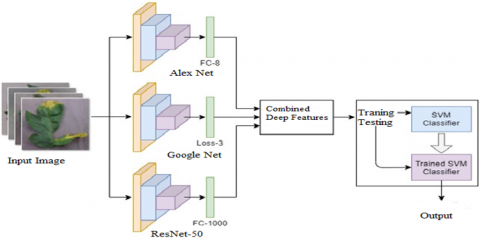
In addition to boost prediction performance, a deep learning model with the purpose of combines’ deep features from three CNN models has been presented. The entire structure of the model that is being suggested can be seen and demonstrated in Figure 2.
Figure 2. Structure of the complete proposed model
Underneath, we present a brief summary of their pre-trained CNN models employed in the analysis. AlexNet [24] is an early architecture for CNNs. The basic structure of AlexNet comprises of 3 completely connected layers and 5 convolution layers.
GoogLeNet [25] is an extension of the inception network that employs a 22-layer CNN structure. Google Net’s most distinctive feature is its innovative implementation of the inception module. All this module does is creating a simple connection between several levels. This raises the bar for network complexity while keeping the price of computation constant.
There are 50 levels in ResNet-50 [26] architecture. ResNet-50 stands itself from competing systems thanks to its modular, micro-level design. It is possible to skip over the transition between some architectural layers and directly access the bottom layer. By permitting transition operations between blocks with this structure, the performance rate of ResNet architecture was able to be boosted.
2.3 Support vector machines
For the sake of putting to use the data gleaned by deep feature extraction, a classifier algorithm must be trained on that data. This research employed an SVM classifier, as proposed by Vapnik [27]. Reports indicate that the SVM classifier excels at a variety of agricultural image classification issues [28].
Finding a hyper plane that optimally separates samples into two groups is the first step in using SVM to solve a classification problem. Eq. (1) gives the formula for the linear SVM's output, where w denotes the normal vector towards the hyper plane and x denotes the input vector. Maximize profits preserve the thought of at the same time as optimization issue, using Eq. (3), where yi and xi are the proper SVM output and input vector for the ith training sample, respectively, and the goal is to minimise Eq. (2) [29].
$u=w\overrightarrow{{}}\cdot x\overrightarrow{{}}-\text{b}$ (1)
$\frac{1}{2}\|w\overrightarrow{{}}\|2$ (2)
$(w\overrightarrow{{}}\cdot x\overrightarrow{{}}i-b)\ge 1,\forall i$ (3)
Support Vector Machine (SVM) be the one of the binary classifiers, meaning it is designed to distinguish between only two classes and does not provide help for multi-class classification issues. Using a 1-to-1 lay down of classifiers to forecast the group picked by the majority of classifiers is one approach to multi-class classification with SVMs [30]. Because the data set used for training each classifier will be less extensive, the amount of time spent on training the classifiers could be reduced.
The deep feature extraction method was utilised in this research to identify pests and diseases affecting tomato plants; this method is a transfer learning strategy that makes use of pre-trained CNN models are extracting the features. The deep features were extracted from the corresponding fully connected layers: FC-1000 for ResNet-50, FC-8 for AlexNet and Loss-3 for GoogLeNet and provided the deep features. Additionally, a model was presented using deep learning to combine 1000 deep characteristics from each of the three CNN models for improved prediction performance. During its training phase, the SVM classifier benefited from the obtained deep features. No custom settings are made for the SVM; all parameters are left at their default values. The i5-8550U CPU, 16GB RAM, 2GB GPU, and 240SDD were utilised in the experiments. All experiments were run in the MATLAB 2019b environment.
The dataset contains a sufficient number of images for a 1-to-1 comparison of the models using the hold-out validation technique. The dataset was split into the two equal parts; the first one is for training and the second one for the testing. When comparing models, we used metrics including accuracy (Accu.), precision (Prec.), sensitivity (Sens.), and F-Score. True positive is defined as TP, FN as abbreviated the false negative, FP as abbreviated the false positive, and as well as true negative is defined as TN are acquired from the confusion matrix and used to compute these performance metrics. The following are the mathematical expressions of the performance metrics used in model comparisons:
$ACCURACY(Accu.)=\frac{T P+T N}{T P+F N+F P+T N}$ (4)
$PRECISION(Prec.)=\frac{T N}{T N+F P}$ (5)
$SENSITIVITY(Sens.)=\frac{T P}{T P+F N}$ (6)
$F-S C O R E=\frac{2 T P}{2 T P+F P+F N}$ (7)
Typically, confusion matrix implications and performance indicators are computed independently for every class in multi-class classification problems. Performance measurements are only meaningful when applied to samples that belong to the class being measured. Following this, the model predictions are used to determine the TP, FN, FP, and TN indices for the representatives that were initially classified as positive and negative.
The dataset samples that have been annotated as Healthy are deemed positive although TP, FN, FP, and TN values are computed on behalf of the healthy class images. The TP value is equal to the count of test set samples that match the Healthy model's prediction. Number of tests set positive samples not anticipated as Healthy by the model constitutes FN. The number of unhealthy samples that were correctly predicted by the model from within the test set is equal to the false positive that is denoted by FP. The number of samples from the test set that were unexpectedly unhealthy is equivalent to the true negative that is denoted by TN of the model.
That is whether or not they were accurately predicted in their own class, any samples outer of the class the confusion matrix indexes are determined are labeled as TN that is negative. Accuracy and sensitivity are both improved by this circumstance.
The total accuracy benchmark is also used to estimate the effectiveness of a model in multi-class classification issues. The proportion of the model's predictions that came true is calculated using this statistic. What follows is the formula for determining that amount.
${Overall}\,{Acc}=\frac{\sum_{i=1}^N T p i}{\sum_{I=1}^N(T p i+F p i)}$ (8)
Here n represents the total figure of categories in the formula. The ith class's accurate prediction is displayed by TPi, while the incorrect prediction is shown by FPi.
Table 2 shows the outcomes of our classification efforts. The table lists the confusion matrix (TP, FN, FP, and TN), accuracy, precision, recall, and sensitivity, as well as the F-Score and overall accuracy (Overall Acc.)
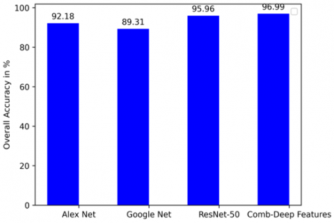
Experiments show that using the SVM classifier to categorise features of deep learning is taken from the final fully connected layers of the CNN models, that are first AlexNet, second GoogLeNet, and the third model is ResNet-50, all are pre-trained CNNs, that yields overall accuracy rates of 92.18%, 89.31%, and 96.96%. All of the CNN models tested in this investigation achieved excellent classification accuracy. However, the overall accuracy of 96.99% has been attained by concatenating deep features, resulting in the best performance. This combined accuracy outperforms the best individual CNN models.
The Accuracy performance comparison of the deep learning algorithms is exposed in the Figure 3. The AlexNet accuracy is starting at 97.07% and the maximum accuracy of recognition is 99.47%. The GoogLeNet accuracy is begin at 96.62% and reached to the maximum is 99.12%. The ResNet model is also same the minimum is 98.7% and maximum is 99.73% accuracy. We proposed model the maximum accuracy is 99.81% and minimum is 99.04% because of combined the deep features and efficient training, testing techniques used here.
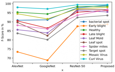
The precision comparison between deep learning algorithms is made known in the Figure 4. Then the AlexNet precision is starting at 98.37% and the maximum precision of prediction is 99.58%. The GoogLeNet precision is begin at 98.24% and reached to the maximum is 99.45%. The ResNet model is also same the minimum is 99.22% and maximum is 99.83% precision. We proposed model the maximum precision is 99.33% and minimum is 99.92% because of combined the deep features of ResNet, GoogleNet and AlexNet models and effective training, testing techniques applied. As same as sensitivity and F-Score performances are high in our proposed model when compared to the remaining models, the graph charts are shown in the Figure 5 and Figure 6.
Extraction of deep features of 3762 test imageset and save the consequential deep feature vector values to disk seeing that a separate new file took 13 minutes 12 seconds for AlexNet, 19 minutes 15 seconds for GoogLeNet, and 49 minutes 58 seconds for ResNet-50. The Overall evaluation of the AlexNet, GoogLeNet, ResNet-50 and we proposed method combined deep features algorithm is shown in the bar chart Figure 7.
Figure 3. Accuracy of different deep learning algorithms
Table 2. Results of classification
|
CNN Model |
Class |
TP |
FN |
FP |
TN |
Accu. (%) |
Prec. |
Sens. |
F-Sco |
Final Acc. (%) |
|
AlexNet |
Bacterial spot |
398 |
25 |
55 |
3318 |
97.89 |
98.37 |
94.09 |
90.87 |
92.18 |
|
Healthy |
303 |
15 |
15 |
3342 |
99.18 |
99.55 |
95.28 |
95.28 |
||
|
Leaf mold |
170 |
24 |
33 |
3548 |
98.49 |
99.08 |
87.63 |
85.64 |
||
|
Late blight |
347 |
37 |
36 |
3462 |
98.12 |
98.97 |
90.36 |
90.48 |
||
|
Early blight |
152 |
55 |
55 |
3512 |
97.09 |
98.46 |
73.43 |
73.43 |
||
|
Sep. leaf spot |
325 |
40 |
35 |
3635 |
98.14 |
99.05 |
89.04 |
89.66 |
||
|
Mosaic Virus |
187 |
7 |
15 |
3560 |
99.42 |
99.58 |
96.39 |
94.44 |
||
|
Target spot |
243 |
56 |
39 |
3430 |
97.48 |
98.88 |
81.27 |
83.65 |
||
|
Spider mites |
296 |
40 |
40 |
3387 |
97.87 |
98.83 |
88.1 |
88.1 |
||
|
Yellow Leaf Curl Virus |
1050 |
16 |
27 |
2678 |
98.86 |
99 |
98.5 |
97.99 |
||
|
GoogLeNet |
Bacterial spot |
385 |
39 |
36 |
3250 |
97.98 |
98.9 |
90.8 |
91.12 |
89.31 |
|
Healthy |
299 |
17 |
19 |
3426 |
99.04 |
99.45 |
94.62 |
94.32 |
||
|
Leaf mold |
169 |
32 |
33 |
3530 |
98.27 |
99.07 |
84.08 |
83.87 |
||
|
Late blight |
320 |
45 |
55 |
3341 |
97.34 |
98.38 |
87.67 |
86.49 |
||
|
Early blight |
140 |
68 |
59 |
3495 |
96.62 |
98.34 |
67.31 |
68.8 |
||
|
Sep. leaf spot |
294 |
66 |
60 |
3341 |
96.65 |
98.24 |
81.67 |
82.35 |
||
|
Mosaic Virus |
180 |
13 |
20 |
3550 |
99.12 |
99.44 |
93.26 |
91.6 |
||
|
Target spot |
226 |
58 |
54 |
3423 |
97.02 |
98.45 |
79.58 |
80.14 |
||
|
Spider mites |
289 |
49 |
45 |
3378 |
97.5 |
98.69 |
85.5 |
86.01 |
||
|
Yellow Leaf Curl Virus |
1040 |
29 |
32 |
2660 |
98.38 |
98.81 |
97.29 |
97.15 |
||
|
ResNet-50 |
Bacterial spot |
413 |
8 |
11 |
3328 |
99.49 |
99.67 |
98.1 |
97.75 |
95.96 |
|
Healthy |
312 |
4 |
6 |
3439 |
99.73 |
99.83 |
98.73 |
98.42 |
||
|
Leaf mold |
192 |
7 |
8 |
3505 |
99.6 |
99.77 |
96.48 |
96.24 |
||
|
Late blight |
367 |
22 |
14 |
3355 |
99.04 |
99.58 |
94.34 |
95.32 |
||
|
Early blight |
172 |
21 |
28 |
3540 |
98.7 |
99.22 |
89.12 |
87.53 |
||
|
Sep. leaf spot |
343 |
11 |
11 |
3396 |
99.42 |
99.68 |
96.89 |
96.89 |
||
|
Mosaic Virus |
192 |
4 |
7 |
3550 |
99.71 |
99.8 |
97.96 |
97.22 |
||
|
Target spot |
255 |
20 |
22 |
3462 |
98.88 |
99.37 |
92.73 |
92.39 |
||
|
Spider mites |
325 |
22 |
22 |
3402 |
98.83 |
99.36 |
93.66 |
93.66 |
||
|
Yellow Leaf Curl Virus |
1064 |
6 |
6 |
2682 |
99.68 |
99.78 |
99.44 |
99.44 |
||
|
Combined Deep Features |
Bacterial spot |
420 |
3 |
4 |
3332 |
99.81 |
99.88 |
99.29 |
99.17 |
96.99 |
|
Healthy |
313 |
4 |
5 |
3456 |
99.76 |
99.86 |
98.74 |
98.58 |
||
|
Leaf mold |
189 |
7 |
11 |
3552 |
99.52 |
99.69 |
96.43 |
95.45 |
||
|
Late blight |
367 |
14 |
14 |
3364 |
99.26 |
99.59 |
96.33 |
96.33 |
||
|
Early blight |
176 |
21 |
24 |
3538 |
98.8 |
99.33 |
89.34 |
88.66 |
||
|
Sep. leaf spot |
346 |
15 |
8 |
3389 |
99.39 |
99.76 |
95.84 |
96.78 |
||
|
Mosaic Virus |
197 |
5 |
3 |
3552 |
99.79 |
99.92 |
97.52 |
98.01 |
||
|
Target spot |
261 |
17 |
19 |
3461 |
99.04 |
99.45 |
93.88 |
93.55 |
||
|
Spider mites |
327 |
13 |
9 |
3411 |
99.41 |
99.74 |
96.18 |
96.75 |
||
|
Yellow Leaf Curl Virus |
1062 |
4 |
8 |
2684 |
99.68 |
99.7 |
99.62 |
99.44 |
Figure 4. Precision of different deep learning algorithms
Figure 5. Sensitivity of different deep learning algorithms
Figure 6. F-Score of different deep learning algorithms
Figure 7. Overall performance accuracy of different deep learning algorithms
Experiments reveal that it is more time-consuming to extract deep features from CNN models by a more no. of layers. Although our system performs admirably in the evaluated cases, it does encounter problems in a few instances, which could be the subject of future research. Because of the scarcity of samples, some classes with high pattern variation are frequently confused with others, resulting in false positives or reduced average accuracy.
There is inconsistency among comparable studies in terms of the total number of categories examined. There was a total of five groups in the study by Sardogan et al. [14], four of which represented disorders and one representing the healthy population. In their study, Rangarajan et al. [15] used seven groups, six of which represented disorders and one representing the healthy population at large. Ten classes were used in these and similar research, with one healthy and nine diseased. This is because the PlantVillage dataset does not contain pre-defined test samples, hence that test samples utilised in similar studies not yet comparable. There is a disparity in the number of samples used for analysis. When working with 600 photos in total, Sardogan et al. [14] split them into two sets: 400 for training and 100 for testing. In their study with a total of 17,600 photos, Agarwal et al. [17] used 10,000 for training, 7,000 images used for validation, and 600 images used for testing. Due to the aforementioned factors, direct comparisons between the relevant studies are impossible.
The performance outcomes of earlier studies that used related datasets were compared in the current study to the combined deep features and SVM method, and these comparative results are shown in Table 3. We give a comparison based on multiple parameters includes the existing methods, type of crops, used method, no. of classes used and total accuracy.
Table 3. Proposed model vs. existing studies
|
Existing study |
Type & class of crop |
Used algorithm |
Total Acc. (%) |
|
Fuentes et al. [12] |
Tomato (10 classes) |
Based on the region CNN |
83.60 |
|
Durmuş et al. [13] |
Tomato (10 classes) |
Retraining a scratch pre-trained CNN model |
95.65 |
|
Sardoğan et al. [14] |
Tomato (5 classes) |
LVQ algorithm |
86.00 |
|
Rangarajan et al. [15] |
Tomato (7 classes) |
Fine Tuned Pre-trained CNN model |
95.49 |
|
Aversano et al. [16] |
Tomato (10 classes) |
Fine Tuned Pre-trained CNN model |
95.16 |
|
Agarwal et al. [17] |
Tomato (10 classes) |
CNN |
91.20 |
|
Saeed et al. [18] |
Tomato (9 classes) Potato (4 classes) Corn (6 classes) |
Deep features selector by PLS-based & an all together belongings tree classifier |
87.11 91.67 91.67 |
|
This study |
Tomato (10 classes) |
Combined deep features and SVM |
96.99 |
This study aimed to explore the potential of using deep feature extraction for recognizing pests and diseases in tomato plants. To achieve this, we utilized well-known pre-trained convolutional neural network (CNN) models, including AlexNet, GoogLeNet, and ResNet-50. By extracting deep features from the final fully connected layers of these CNN models, a total of 1000 deep features were utilized to improve the capabilities of the SVM classifier. We developed a deep learning technique that combined the 1000 deep features from each of the three CNN models to enhance prediction accuracy. Experimental results demonstrated that while using deep features from each individual CNN model yielded good classification performance, the best results were achieved by combining information from multiple models. This could be attributed to the fact that different CNN model topologies reveal distinct sets of discriminative characteristics. The ultimate goal of this research is to identify diseases in tomato plant leaves and provide recommendations regarding suitable pesticides for field spraying, while also enhancing the classification performance compared to other CNN algorithms. Additionally, the efficiency of the constructed models will be assessed by testing them on real-world photographs taken under realistic conditions.
[1] Mohanty, S.P., Hughes, D.P., Salathé, M. (2016). Using deep learning for image-based plant disease detection. Frontiers in Plant Science, 7: 1419. https://doi.org/10.3389/fpls.2016.01419
[2] Ferentinos, K.P. (2018). Deep learning models for plant disease detection and diagnosis. Computers and Electronics in Agriculture, 145: 311-318. https://doi.org/10.1016/j.compag.2018.01.009
[3] Al-Hiary, H., Bani-Ahmad, S., Reyalat, M., Braik, M., Alrahamneh, Z. (2011). Fast and accurate detection and classification of plant diseases. International Journal of Computer Applications, 17(1): 31-38. https://doi.org/10.5120/2183-2754
[4] Dubey, S.R., Jalal, A.S. (2012). Detection and classification of apple fruit diseases using complete local binary patterns. In 2012 Third International Conference on Computer and Communication Technology. IEEE, pp. 346-351. https://doi.org/10.1109/ICCCT.2012.76
[5] Singh, V., Misra, A.K. (2017). Detection of plant leaf diseases using image segmentation and soft computing techniques. Information Processing in Agriculture, 4(1): 41-49. https://doi.org/10.1016/j.inpa.2016.10.005
[6] LeCun, Y., Bengio, Y., Hinton, G. (2015). Deep learning. Nature, 521(7553): 436-444. https://doi.org/10.1038/nature14539
[7] Ünal, Z. (2020). Smart farming becomes even smarter with deep learning-a bibliographical analysis. IEEE Access, 8: 105587-105609. https://doi.org/10.1109/ACCESS.2020.3000175
[8] Kamilaris, A., Prenafeta-Boldú, F.X. (2018). Deep learning in agriculture: A survey. Computers and Electronics in Agriculture, 147: 70-90. https://doi.org/10.1016/j.compag.2018.02.016
[9] Zhong, Y., Zhao, M. (2020). Research on deep learning in apple leaf disease recognition. Computers and Electronics in Agriculture, 168: 105146. https://doi.org/10.1016/j.compag.2019.105146
[10] Fujita, E., Kawasaki, Y., Uga, H., Kagiwada, S., Iyatomi, H. (2016). Basic investigation on a robust and practical plant diagnostic system. In 2016 15th IEEE International Conference on Machine Learning and Applications (ICMLA), pp. 989-992. https://doi.org/10.1109/ICMLA.2016.0178
[11] Lu, Y., Yi, S., Zeng, N., Liu, Y., Zhang, Y. (2017). Identification of rice diseases using deep convolutional neural networks. Neurocomputing, 267: 378-384. https://doi.org/10.1016/j.neucom.2017.06.023
[12] Fuentes, A., Yoon, S., Kim, S.C., Park, D.S. (2017). A robust deep-learning-based detector for real-time tomato plant diseases and pests recognition. Sensors, 17(9): 2022. https://doi.org/10.3390/s17092022
[13] Durmuş, H., Güneş, E.O., Kırcı, M. (2017). Disease detection on the leaves of the tomato plants by using deep learning. In 2017 6th International Conference on Agro-Geoinformatics. IEEE, pp. 1-5. https://doi.org/10.1109/Agro-Geoinformatics.2017.8047016
[14] Sardogan, M., Tuncer, A., Ozen, Y. (2018). Plant leaf disease detection and classification based on CNN with LVQ algorithm. In 2018 3rd International Conference on Computer Science and Engineering (UBMK). IEEE, pp. 382-385. https://doi.org/10.1109/UBMK.2018.8566635
[15] Rangarajan, A.K., Purushothaman, R., Ramesh, A. (2018). Tomato crop disease classification using pre-trained deep learning algorithm. Procedia Computer Science, 133: 1040-1047. https://doi.org/10.1016/j.procs.2018.07.070
[16] Aversano, L., Bernardi, M.L., Cimitile, M., Iammarino, M., Rondinella, S. (2020). Tomato diseases classification based on VGG and transfer learning. In 2020 IEEE International Workshop on Metrology for Agriculture and Forestry (MetroAgriFor), pp. 129-133. https://doi.org/10.1109/MetroAgriFor50201.2020.9277626
[17] Agarwal, M., Singh, A., Arjaria, S., Sinha, A., Gupta, S. (2020). ToLeD: Tomato leaf disease detection using convolution neural network. Procedia Computer Science, 167: 293-301. https://doi.org/10.1016/j.procs.2020.03.225
[18] Saeed, F., Khan, M.A., Sharif, M., Mittal, M., Goyal, L.M., Roy, S. (2021). Deep neural network features fusion and selection based on PLS regression with an application for crops diseases classification. Applied Soft Computing, 103: 107164. https://doi.org/10.1016/j.asoc.2021.107164
[19] Hughes, D., Salathé, M. (2015). An open access repository of images on plant health to enable the development of mobile disease diagnostics. arXiv Preprint arXiv: 1511.08060. https://doi.org/10.48550/arXiv.1511.08060
[20] Geetharamani, G., Pandian, A. (2019). Identification of plant leaf diseases using a nine-layer deep convolutional neural network. Computers & Electrical Engineering, 76: 323-338. https://doi.org/10.1016/j.compeleceng.2019.04.011
[21] Altuntaş, Y., Cömert, Z., Kocamaz, A.F. (2019). Identification of haploid and diploid maize seeds using convolutional neural networks and a transfer learning approach. Computers and Electronics in Agriculture, 163: 104874. https://doi.org/10.1016/j.compag.2019.104874
[22] Chatfield, K., Simonyan, K., Vedaldi, A., Zisserman, A. (2014). Return of the devil in the details: Delving deep into convolutional nets. arXiv Preprint arXiv: 1405.3531. https://doi.org/10.48550/arXiv.1405.3531
[23] Toğaçar, M., Ergen, B., Cömert, Z. (2020). Classification of flower species by using features extracted from the intersection of feature selection methods in convolutional neural network models. Measurement, 158: 107703. https://doi.org/10.1016/j.measurement.2020.107703
[24] Krizhevsky, A., Sutskever, I., Hinton, G.E. (2012). Imagenet classification with deep convolutional neural networks. Advances in Neural Information Processing Systems, 25.
[25] Szegedy, C., Liu, W., Jia, Y., Sermanet, P., Reed, S., Anguelov, D., Erhan, D., Vanhoucke, V., Rabinovich, A. (2015). Going deeper with convolutions. In Proceedings of the IEEE Conference on Computer Vision and Pattern Recognition, pp. 1-9. https://doi.org/10.48550/arXiv.1409.4842
[26] He, K., Zhang, X., Ren, S., Sun, J. (2016). Deep residual learning for image recognition. In Proceedings of the IEEE Conference on Computer Vision and Pattern Recognition, pp. 770-778. https://doi.org/10.48550/arXiv.1512.03385
[27] Vapnik, V.N. (2000). The nature of statistical learning theory. New York, NY: Springer.
[28] Huang, S., Cai, N., Pacheco, P.P., Narrandes, S., Wang, Y., Xu, W. (2018). Applications of support vector machine (SVM) learning in cancer genomics. Cancer Genomics & Proteomics, 15(1): 41-51. https://doi.org/10.21873/cgp.20063
[29] Bishop, C.M., Nasrabadi, N.M. (2006). Pattern recognition and machine learning. New York: Springer, 4(4): 738.
[30] Agarwal, M., Singh, A., Arjaria, S., Sinha, A., Gupta, S. (2020). ToLeD: Tomato leaf disease detection using convolution neural network. Procedia Computer Science, 167: 293-301. https://doi.org/10.1016/j.procs.2020.03.225