Istiqomah*![]() | Achmad Rizal
| Achmad Rizal![]() | Ratri Dwi Atmaja
| Ratri Dwi Atmaja![]()
© 2023 IIETA. This article is published by IIETA and is licensed under the CC BY 4.0 license (http://creativecommons.org/licenses/by/4.0/).
OPEN ACCESS
The way a person walks has unique characteristics for each individual and can be used to recognize them. There are various ways to classify characteristics for gait of each individual, one of them is the inertia sensor. The inertia sensor is used to collect data gait signals, which are angular velocity variations caused by human walking movements. Multi-distance Signal Level Difference Sample Entropy is proposed in this study as a feature extraction before classifying individual gaits. MSLD is used to measure the co-occurrence of two signal samples at a distance d, and SampEn quantizes signal complexity. The MSLD Entropy produce 60 features in the form of SampEn at distances of 1 until 20 from the three-axis. The testing procedure is carried out on the MSLD Entropy result signal for each classifier with a feature in the form of SampEn at distances of d=1–20, d=1–15, d=1–10, and d=1–5. Softmax regression as a classifier and feature at distance 1 until 20, the test results produce the greatest accuracy of 98.3%. Because a person's gait can be identified not just from one but three directions, using only one axis results in lesser accuracy than using data from all three axes.
individual recognition, gait, inertia sensor, MSLD entropy
The way a person walks has characteristics for each individual, influenced by weight, foot length, foot width, and body posture combined with each individual's gait characteristics. The difference in gait can be used as a biometric measure to identify a person, recognize unknown subjects, and even represent a person's overall path by adding other aspects of the parameter [1].
Various ways can be done to identify a person's gait. In this research [1], gait representation is taken from a video of human walking movement, which is extracted from the orthogonal silhouette of the walking movement. Different ways can be done [2] by examining the similarity of a person's self-image while walking. Sensors are used for gait analysis using video or image is Microsoft Kinect [3] or surveillance cameras [4]. Another method used is by utilizing inertia sensors to obtain changes in angular velocity from human walking movements. Inertia sensors have excess, such as smaller, lighter, cheaper, less power consumption, and easy to use; even inertia sensors are embedded in smartphones [5, 6].
Several approaches have been developed for the feature extraction process on the gait signal from the inertia sensor. One of the popular techniques for gait analysis is entropy [7]. The entropy used for gait analysis includes sample entropy (SamEn) [8], dispersion entropy [9]. Entropy is used for gait analysis because it quantifies the regularity or irregularity of a series of signals in the time domain. The regularity of the gait signal from this inertia sensor can be distinguished through entropy analysis.
The previous study [10, 11] proposed the Multidistance Signal Level Difference (MSLD) as a combination with sample entropy for future extraction. MSLD is a one-dimensional signal decomposition method that calculates the absolute value of the difference in signal samples at a certain distance [10]. The result of the signal from the MSLD process is calculated as its entropy and becomes an input to the classification process. MSLD entropy has been shown to produce high accuracy with average 97% in case EEG signal and Lung sound analysis [10, 11]. Because of the good performance of MSLD entropy in the previous case, in this research, the Multidistance Signal Level Difference Sample Entropy (MSLD Entropy) method is proposed for individual recognition based on the gait signal generated from the inertia sensor. It is expected that this method will also produce high accuracy for classifying individuals based on gait using an inertia sensor. This paper will elaborate about propose method of the research, the gather gait dataset, feature extraction algorithm, classification method, result dan discussion, and conclusion.
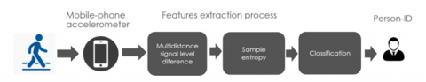
Figure 1 is a picture of the method proposed in this study. First, the individual gait data retrieval process is carried out. Then continue with the feature extraction process from the gait signal. The last is the process of classifying the introduction of gait from the subject using machine learning methods. A detailed description of each process is presented below.
Individual gait data were collected using a gyroscope sensor on a smartphone placed on the right quadriceps. The feature extraction process is carried out using multidistance signal level difference and sample entropy from the signal data obtained. Then perform various classifications using various methods and 5-fold cross-validation to avoid overfitting [12]. Machine learning methods used include AdaBoost, Stochastic Gradient Descent (SGD), Gradient Boosting, Random Forest, Decision Tree (DT), Gaussian Naïve Bayes, KNN, SVM, and Softmax Regression [13]. A detailed description of each process is presented in the following subsections.
Figure 1. Proposed method
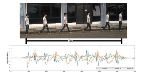
Data acquisition of gait is captured using the gyroscope sensor on the Xiaomi Redmi 1S smartphone. Data were obtained from 30 people, and every person is taken 12 signal data [6]. The sampling frequency used is 50 Hz with a recording length of 14 seconds. A person whose gait data is taken is attached to a smartphone on the right quadriceps, as shown in Figure 2. The data recording process is carried out in a way, the person walks 5 m, and the acceleration gait data is taken for the X-Axis, Y-Axis, Z- Axis, which can be illustrated in Figure 3.
Figure 2. Mobile phone as data acquisition tool and configuration
Figure 3. Illustration of gait data recording and accelerometer gait signal
This section elaborates algorithm multi-distance signal level distance Sample Entropy (MSDL Entropy) as feature extraction and classifier method. MSDL Entropy is feature extraction which combination from Multi-distance Signal Level Distance and Sample Entropy. Features which be produced, then be classified with some machine learning method, such as AdaBoost, Stochastic Gradient Descent (SGD), Gradient Boosting, Random Forest, Decision Tree (DT), Gaussian Naïve Bayes, KNN, SVM, and Softmax Regression.
4.1 Multi-distance signal level distance
Weszka et al. [14] compare texture measures with various feature classes, one of them is the gray-level difference (GLD). GLD is calculated using the absolute value of the discrepancy between two nearby pixels in the three dimensions: horizontal, vertical, and diagonal. GLD calculates one dimension signal. Whereas Multidistance signal level difference (MSLD) is a modification of gray-level difference(GLD) become multidistance. Eq. (1) is used to determine GLD in the horizontal direction, with D is distance between pixels. That formula is modified for MSLD in Eq. (2), by change pixels distance into distance index of data. Figure 4 illustrates the MSLD process for scale distance 1, 2, and 3.
$\begin{gathered}y(i, j)=|x(i, j)-x(i, j+D)| \\ D=\text { pixel distance }\end{gathered}$ (1)
$\begin{gathered}y_d(i)=|x(i)-x(i+d)| \\ i=1,2, \ldots, N-d \text { and } d=1,2, \ldots, K\end{gathered}$ (2)
Figure 4. MSLD proces
4.2 Sample entropy
To address ApEn's flaws, Richman and Moorman introduced sample entropy (SampEn) [15]. Because the signal's code template is deemed the same as itself, there is bias due to self-matches in ApEn. SampEn is the probability measure that a sequence of m data will be identical to another sequence in a signal sequence with a tolerance of r and that the sequence of m data will remain identical if the series of m data is increased to m+1. In this scenario, the two vectors being compared have a scalable distance between them [16]. Mathematically SampEn is expressed by Eq. (3).
$\operatorname{SampEn}(m, r)=\lim _{N \rightarrow \infty}-\ln \frac{A^m(r)}{B^m(r)}$ (3)
The probability will resemble that two sequences for a number of m+1 points within a tolerance of r are denoted Am(r). Bm(r) has a similar definition of probability and tolerance with Am(r) but with the number of m points difference, self-matches are avoided in both parameters. Furthermore, Eq. (3) can be simplify by substitute variable with Eq. (4) and Eq. (5) and so that SampEn can be expressed by Eq. (6).
$B=\{[(N-m-1)(N-m)] / 2\} B^m(r)$ (4)
And
$A=\left\{\frac{[(N-m-1)(N-m)]}{2}\right\} A^m(r)$ (5)
In addition, SampEn can be written as a formula (6)
$\operatorname{SampEn}(m, r, N)=-\ln \frac{A}{B}$ (6)
The following are some of the advantages of SampEn: It could be used for short data series and yet contain noise, it can distinguish huge system variations, it has better performance than ApEn, it has constant entropy values for various pattern lengths, and it does not calculate self-match. The inconsistency of entropy levels for short data is one of SampEn's weaknesses [17].
4.3 Classifier
The classifiers used in previous research [1, 4], namely SVM and KNN, have good performance in the classification process, which was later used in this study. However, in addition to using these two classifiers, this research also utilizes other classifiers, namely AdaBoost, Stochastic Gradient Descent, Gradient Boosting, Random Forest, Decision Tree, Gaussian Naive Bayes, and Softmax Regression [13]. Gait recognition results from each classifier are compared to get the best classifier in this method.
4.4 K-fold Cross-Validation
In machine learning, data used for training cannot be used for validation models. As a result, the data is divided into two pieces at the start of the process: train data and test data, which are utilized in the training and model evaluation phases, respectively. However, the training data is reduced as a result of this validation process [13]. So that the test data can still be used for the training process, in this study, cross-validation was used to validate the machine learning model.
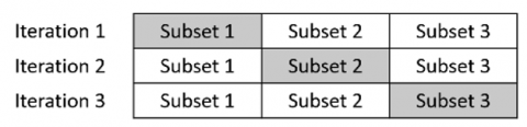
Figure 5. Illustration of 3-fold
The dataset is divided into several parts according to the desired number of K-folds for process cross-validation. One subset of the data is chosen as the validation dataset during an iteration of the training process, while the other is used for the training data. For the validation dataset, each iteration step utilizes a different subset. The training procedure is repeated until the complete subset has been used to validate the process. The 3-fold cross-validation was employed in this study, as shown in Figure 5. The selection of 3-fold validation is based on the fact that the training set and validation set have a more balanced size for data sizes that are not large.
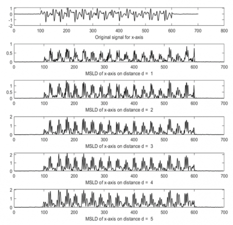
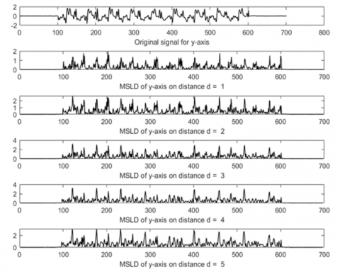
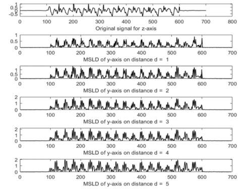
Figure 6, Figure 7, and Figure 8 show examples of MSLD processing results on subject number one on the X-Axis, Y-Axis, Z-Axis, respectively. Because of the absolute sign in Eq. (2), the signal from the MSLD result becomes positive. The shape of the MSLD process signal tends to stay the same for the value of d=1–5 because the sampling frequency is 50 Hz. Meanwhile, the change in the sensor signal changes relatively slowly, considering the normal walking pattern of the subject. With a sampling frequency of 50 Hz, the distance d=1 represents a sampling period of 0.01 seconds, while a normal running cycle is 1.2–1.5 meters per second [18]. With a distance of d=1–5, the data sample distance is up to 0.05 seconds, resulting in the difference in the MSLD signal at d=1–5 does not look significantly different visually. This difference could be seen in the SampEn calculation process in the next process.
Figure 6. Original signal for x-axis and MSLD result for d=1–5
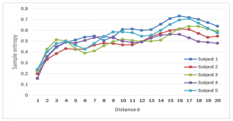
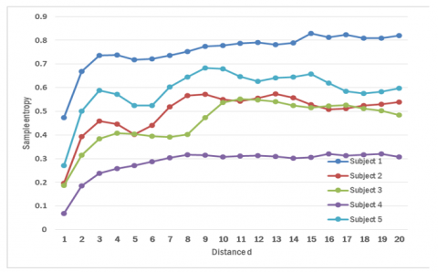
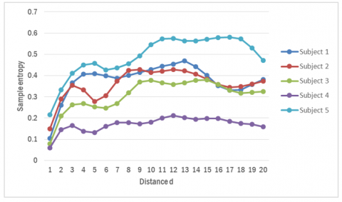
Figure 9, Figure 10, and Figure 11 show the mean scores of the five subjects on the X-Axis, Y-Axis, Z-Axis. The SampEn value tends to increase as the distance d additions from 1-16 and then decreases. The characteristics of the five subjects look different even though the values are a bit close together. The entropy value increases at a more significant distance due to the difference between samples' greater value in the MSLD process, resulting in higher signal fluctuations.
Figure 7. Original signal for y-axis and MSLD result for d=1–5
The subject's stance time (temporal symmetry), stride length when stepping (spatial symmetry), and limit motion of hip and knee (kinematic symmetry) can be used to determine the different patterns of each subject [19]. This difference will make a change in the value captured by the sensor. The walking rate affects the speed of signal change and makes the MSLD process signal change faster. It makes the SampEn value also change so that it can be used to distinguish between one subject and another.
Figure 8. Original signal for z-axis and MSLD result for d=1–5
Figure 9. Features of five subjects at x axis
Figure 10. Features of five subjects at y axis
Figure 11. Features of five subjects at z axis
The testing procedure is carried out on the MSLD result signal for each classifier with a feature in the form of SampEn at distances of d=1–20, d=1–15, d=1–10, and d=1–5. Table 1, Table 2, Table 3, and Table 4 exhibit the accuracy findings. Table 1 shows the accuracy when all three axes' characteristics are utilized together, whereas Tables 2, 3, and 4 show the accuracy when the X-Axis, Y-Axis, Z-Axis features are employed separately. When three three-axis characteristics are employed concurrently, the greatest accuracy is reached, which is 98.3 percent using Softmax Regression. Meanwhile, the x-axis with Softmax Regression as a classifier produces the highest accuracy of 89.7% when features on one axis are used. Both findings were obtained with d=1–20, indicating that more features lead to greater accuracy. This can be seen in all tables, where the higher the accuracy, the more features are used. The usage of the distance d=1–20 on the X-Axis, Y-Axis, Z-Axis means that the classification uses 60 different features.
Table 1. Accuracy (%) for each classifier using X-Y-Z axis and 3-fold CV
|
Classifier |
Distance d=1-20 |
Distance d=1-15 |
Distance d=1-10 |
Distance D=1-5 |
|
AdaBoost |
51.9% |
51.1% |
44.7% |
44.7% |
|
Stochastic Gradient Descent |
41.9% |
41.7% |
29.7% |
32.2% |
|
Gradient Boostin |
75.8% |
73.1% |
70.8% |
70.5% |
|
Random Forest |
92.7% |
91.4% |
84.4% |
86.1% |
|
KNN |
94.7% |
95.3% |
86.3% |
86.3% |
|
Decision Tree |
66.1% |
67.8% |
60.5% |
64.1% |
|
Gaussian NB |
76.9% |
73.9% |
63.6% |
63.6% |
|
SVM |
98.0% |
97.2% |
81.4% |
81.3% |
|
Softmax Regression |
98.3% |
97.8% |
81.6% |
81.6% |
Table 2. Accuracy (%) for each classifier using X axis and 3-fold CV
|
Classifier |
Distance d=1-20 |
Distance d=1-15 |
Distance d=1-10 |
Distance D=1-5 |
|
AdaBoost |
30.0% |
21.9% |
18.0% |
15.0% |
|
Stochastic Gradient Descent |
35.2% |
23.6% |
21.1% |
13.6% |
|
Gradient Boostin |
62.2% |
59.1% |
50.2% |
43.6% |
|
Random Forest |
77.2% |
74.1% |
64.1% |
51.3% |
|
KNN |
84.4% |
77.7% |
65.8% |
53.6% |
|
Decision Tree |
57.5% |
54.4% |
45.2% |
41.4% |
|
Gaussian NB |
55.8% |
49.0% |
43.8% |
35.3% |
|
SVM |
86.9% |
76.3% |
52.2% |
38.6% |
|
Softmax Regression |
89.7% |
82.2% |
66.9% |
45.5% |
Table 3. Accuracy (%) for each classifier using Y axis and 3-fold CV
|
Classifier |
Distance d=1-20 |
Distance d=1-15 |
Distance d=1-10 |
Distance D=1-5 |
|
AdaBoost |
24.4% |
20.8% |
16.9% |
13.8% |
|
Stochastic Gradient Descent |
25.3% |
16.9% |
18.9% |
10.3% |
|
Gradient Boostin |
56.7% |
54.4% |
47.2% |
44.1% |
|
Random Forest |
70.0% |
69.1% |
61.1% |
50.5% |
|
KNN |
79.8% |
74.7% |
63.9% |
51.1% |
|
Decision Tree |
50.5% |
50.8% |
47.2% |
43.3% |
|
Gaussian NB |
44.1% |
41.7% |
35.3% |
33.0% |
|
SVM |
80.5% |
67.2% |
50.3% |
32.5% |
|
Softmax Regression |
79.2% |
70.0% |
60.5% |
40.8% |
Table 4. Accuracy (%) for each classifier using Z axis and 3-fold CV
|
Classifier |
Distance d=1-20 |
Distance d=1-15 |
Distance d=1-10 |
Distance D=1-5 |
|
AdaBoost |
28.3% |
26.6% |
22.8% |
18.0% |
|
Stochastic Gradient Descent |
31.1% |
20.0% |
20.0% |
10.8% |
|
Gradient Boostin |
65.5% |
56.9% |
55.8% |
37.8% |
|
Random Forest |
79.1% |
74.4% |
70.0% |
51.9% |
|
KNN |
78.3% |
71.9% |
68.0% |
51.4% |
|
Decision Tree |
58.8% |
55.3% |
53.3% |
42.8% |
|
Gaussian NB |
51.9% |
44.2% |
43.8% |
36.1% |
|
SVM |
74.1% |
61.4% |
46.7% |
33.6% |
|
Softmax Regression |
78.9% |
72.2% |
62.5% |
39.1% |
Previous studies using the same data set get an accuracy of up to 99.58% [6]. The feature extraction method used is Linear Predictive Coding (LPC), commonly used in speech signal processing. The difference is in the use of signal magnitude, which is formulated as $\overline{S m}=\sqrt{\overline{S x}^2+\overline{S y}^2+\overline{S z}^2}$ so that the number of features used is more than the proposed method.
The proposed method has preferences in terms of ease of calculation and does not require signal transformation. MSLD determines the difference between two signal samples to capture events with two data samples. On a periodic signal, the MSLD result becomes zero at a distance d=signal period. Thus differences in one's gait produce different signals. The SampEn quantizes the MSLD signal for each person. The proposed method allows further exploration by changing various parameters such as the number of distances d in MSLD, m series, and tolerance r in SampEn. MSLD also has several variations with some calculation differences [20]. Further research of the use of various variations of MSLD becomes an interesting topic for more research.
This research proposes method a gait analysis feature extraction for biometrics with a gyroscope sensor. The gyroscope sensor used is a gyroscope installed on a mobile phone. Meanwhile, the proposed feature extraction methods are multi-distance signal level difference (MSLD) and sample entropy (SampEn). MSLD is used to measure the co-occurrence of two signal samples at a distance d, and SampEn is used to quantizes signal complexity. The test results produce the highest accuracy of 98.3% using 60 features and Softmax Regression as a classifier. Using one axis only results in lower accuracy than using features of the three axes because a person's gait can be distinguished not only from one direction but three directions. The proposed method still opens opportunities for the exploration of more optimal parameter selection in order to increase accuracy. The use of other MSLD variations can be tried for the feature extraction process in future studies.
[1] Lee, L., Grimson, W.E.L. (2002). Gait analysis for recognition and classification. In Proceedings of Fifth IEEE International Conference on Automatic Face Gesture Recognition, 155-162. https://doi.org/10.1109/AFGR.2002.1004148
[2] BenAbdelkader, C., Cutler, R.G., Davis, L.S. (2004). Gait recognition using image self-similarity. EURASIP Journal on Advances in Signal Processing, 2004(4): 1-14. https://doi.org/10.1155/S1110865704309236
[3] Xu, X., McGorry, R.W., Chou, L.S., Lin, J.H., Chang, C.C. (2015). Accuracy of the Microsoft Kinect™ for measuring gait parameters during treadmill walking. Gait & Posture, 42(2): 145-151. https://doi.org/10.1016/j.gaitpost.2015.05.002
[4] Lee, C.P., Tan, A.W.C., Lim, K.M. (2017). Review on vision-based gait recognition: Representations, classification schemes and datasets. American Journal of Applied Sciences, 14(2): 252-266. https://doi.org/10.3844/ajassp.2017.252.266
[5] Sprager, S., Juric, M.B. (2015). Inertial sensor-based gait recognition: A review. Sensors, 15(9): 22089-22127. https://doi.org/10.3390/s150922089
[6] Annas, M.S., Rizal, A., Atmaja, R.D. (2017). Pengenalan Individu Berdasarkan Gait Menggunakan Sensor Giroskop. Jurnal Nasional Teknik Elektro dan Teknologi Informasi (JNTETI), 6(2): 210-214. https://doi.org/10.22146/jnteti.v6i2.317
[7] Torres, B.D.L.C., López, M.S., Cachadiña, E.S., Orellana, J.N. (2013). Entropy in the analysis of gait complexity: A state of the art. British Journal of Applied Science & Technology, 3(4): 1097. https://doi.org/10.9734/bjast/2014/4698
[8] Ahmadi, S., Sepehri, N., Wu, C., Szturm, T. (2018). Sample entropy of human gait center of pressure displacement: a systematic methodological analysis. Entropy, 20(8): 579. https://doi.org/10.3390/e20080579
[9] Amezquita-Sanchez, J.P., Mammone, N., Morabito, F.C., Adeli, H. (2021). A new dispersion entropy and fuzzy logic system methodology for automated classification of dementia stages using electroencephalograms. Clinical Neurology and Neurosurgery, 201: 106446. https://doi.org/10.1016/J.CLINEURO.2020.106446
[10] Rizal, A., Hidayat, R., Nugroho, H.A. (2017). Hjorth descriptor measurement on multidistance signal level difference for lung sound classification. Journal of Telecommunication, Electronic and Computer Engineering (JTEC), 9(2): 23-27.
[11] Rizal, A., Hadiyoso, S. (2018). Sample entropy on multidistance signal level difference for epileptic EEG classification. The Scientific World Journal, 2018. https://doi.org/10.1155/2018/8463256
[12] Mehrabi, S., Maghsoudloo, M., Arabalibeik, H., Noormand, R., Nozari, Y. (2009). Application of multilayer perceptron and radial basis function neural networks in differentiating between chronic obstructive pulmonary and congestive heart failure diseases. Expert Systems with Applications, 36(3): 6956-6959. https://doi.org/10.1016/j.eswa.2008.08.039
[13] Géron, A. (2017). Hands-on Machine Learning, 53(9).
[14] Weszka, J.S., Dyer, C.R., Rosenfeld, A. (1976). A comparative study of texture measures for terrain classification. IEEE transactions on Systems, Man, and Cybernetics, 4: 269-285. https://doi.org/10.1109/TSMC.1976.5408777.
[15] Richman, J.S., Moorman, J.R. (2000). Physiological time-series analysis using approximate entropy and sample entropy. American Journal of Physiology-Heart and Circulatory Physiology, 278(6): H2039-H2049. https://doi.org/10.1152/ajpheart.2000.278.6.H2039
[16] Humeau-Heurtier, A. (2015). The multiscale entropy algorithm and its variants: A review. Entropy, 17(5): 3110-3123. https://doi.org/10.3390/e17053110
[17] Acharya, U.R., Fujita, H., Sudarshan, V.K., Bhat, S., Koh, J.E. (2015). Application of entropies for automated diagnosis of epilepsy using EEG signals: A review. Knowledge-based systems, 88: 85-96. https://doi.org/10.1016/j.knosys.2015.08.004
[18] Kim, J., Lee, G., Heimgartner, R., Arumukhom Revi, D., Karavas, N., Nathanson, D., Walsh, C.J. (2019). Reducing the metabolic rate of walking and running with a versatile, portable exosuit. Science, 365(6454): 668-672. https://doi.org/10.1126/science.aav7536
[19] Guzik, A., Drużbicki, M., Perenc, L., Podgórska-Bednarz, J. (2020). Can an Observational Gait Scale Produce a Result Consistent with Symmetry Indexes Obtained from 3-Dimensional Gait Analysis? A Concurrent Validity Study. Journal of Clinical Medicine, 9(4): 926. https://doi.org/10.3390/jcm9040926
[20] Rizal, A., Hidayat, R., Nugroho, H.A. (2019). Comparison of multi-distance signal level difference Hjorth descriptor and its variations for lung sound classifications. Indonesian Journal of Electrical Engineering and Informatics (IJEEI), 7(2): 345-356. https://doi.org/10.11591/ijeei.v7i2.771