Venkata Naresh Mandhala | Debnath Bhattacharyya | Divya Midhunchakkaravarthy | Hye-jin Kim*
© 2022 IIETA. This article is published by IIETA and is licensed under the CC BY 4.0 license (http://creativecommons.org/licenses/by/4.0/).
OPEN ACCESS
In this paper, the proposed algorithm to detect the bias from the datasets and to mitigate the bias in the datasets was observed. The consequences of this work shows that not only bias in a model can be decreased without forfeiting model performance rate, but improving the performance. Class imbalance, KL divergence, sample disparity and Kolmogorov-Smirnov (KS) are the pre-training metrics used in the work. Each metric is given weightage and the features are detected based on the maximum weightage. The model is trained to learn the unbiased data and shows the significant improvement in the performance of the system. ROC curve, False Positive Rate and False Negative Rate is used for bias trade-off. The comparison between FPR and FNR before mitigating bias and after mitigating bias is performed and its results are significantly improved.
bias mitigation, class imbalance, KL divergence, sample disparity, KS, ROC curve, FPR, FNR
Development of a basic yet viable AI model requires the capacity to choose just the features that convey the greatest expectation potential. Notwithstanding, when confronted with an informational index involving countless features, an experimentation approach prompts loss of time and handling resources. Generally, for any data analysis applications, the dataset is investigated systematically, and just a subset of features is saved for model choice, along these lines keeping the model basic yet successful.
Normally, during the advancement of the model, one piece of the data is used for validating or testing the model. During this stage ordinarily one needs to check if the model has taken in generalized information. At the end of the model development, it should perform well on data which is not used in the learning stage. In any case, prior to being prepared to utilize the model numerous tests ought to be done to check that the model is right.
We may find that our model in general give ideal forecasts to certain examples and less ideal for other people, in an orderly and inappropriate way. Great on the off chance that we find this issue called bias prior to utilizing the model.
Bias in data may be considered as systematic error. To debug these kinds of errors, first we have to find the bias. Unmitigated biases may weak the insight of objectivity and impartiality in model.
Bias ought to be distinguished before it very well may be tended to. Bias can be recognized by noticing the objective variable effect on the different feature subsets of information. So, Machine learning and Statistical methods are utilized to gauge and identify the bias in the information. So, the main objective of our proposal is to foster a framework to detect and mitigate bias which yields to improve the performance of a model.
In this paper, an algorithm is proposed to detect and also to mitigate the bias in the datasets, it also improves the performance rate. The model identifies the unbiased data by using class imbalance, KL divergence, sample disparity and Kolmogorov-Smirnov (KS) as pre-training metrics. The model is trained to reduce the disparity among the protected variables which are identified by the pre-training metrics.
Collection of data from various sources is an important aspect with respect to the dataset creation or preparation. When it comes to the social media huge amounts of data will be available in the form of likes, post as well as connections which allow people to connect from different parts of the globe. When large volumes of data are collected for analysis from different sources there is a possibility of bias presence in the data. Morstatter [1] proposed that bias can be formed in the social media themselves and mainly age-bias is one of the major aspects with the data.
Data from different sources with different types are always a challenging when we consider it for analysis of biomedical studies. When that type of data was fed to any black-box machine learning techniques it leads to the existing of bias and the results are unpredictable and will not help for better decision making. Venugopalan et al. [2] Considered the data to study in different aspects. One, identifying the bias that is present in the data that was generated due to illegitimate data which may create a nuisance in the results, and the other is due to the type of data that we take that leads to an unpredictable result.
Data in the recommender system helps the customer to choose their products effectively without spending much time. As the recommender system are used to facilitate the selection of products based on the browsing and helps the customers based on the acceptance rate. Social Influence Bias (SIB) is the challenging area in the recommender system. Krishnan et al. [3] proposed the LAM (Learn, Analyze and Mitigate) the effect of SIB. Each face holds a step of procedure to analyze the bias, first we build a dataset based on the rating of the customers and collect twice one before and the other after browsing the average rating.
Empathy is being the major challenging area in artificial intelligence, where detecting the human emotions and analyzing them is the need now a days. In order to perform there is a need of large volumes of data collection is required and the collected data has to be analyzed for accurate recognition of emotions. In this regard there is a chance of bias in the datasets [4].
To reduce the faulty decision making by the employees in the organization relying on a technologies like Artificial Intelligence has emerged and performing well with respect to analyze the problems present in the organization. To overcome the unconscious bias that is present in the organization AI has been delve into the employment decisions mainly to mitigate the bias that was mentioned [5].
Analyzing the data by using the small dataset will not yield good results as per the studies. In order to make our model more predictable to identify the diseases there is a need to large datasets by pooling them from different sources. In this connection Neuroimaging datasets are growing now a days and addressing them is quite difficult because of the bias present in the datasets. Wachinger et al. [6] considered 12,207 MRI images and concluded when considered for training due to the data collection from different sources the bias present in the dataset is high. To overcome this affect various steps have been proposed. First step is to define the cause of bias. Second step is to detect the bias and mitigating them and last step is to override the confounding factors using causal inference.
While considering the features to identify the bias in the databases, geography-based, gender-based and object-based are few metrics that are been considered in computer vision is object-based metrics. In this regard a new concept, Progressive Visualization has become a wide used visualization technique when the large amount of data is considered. By using this technique, the intermediate results can be examined for complex and also long run computations apart from considering the complete computational results. Using this we can take the intermediate results which will benefit the users of the model and also researchers to identify the potential risks that occur due to this. This leads to the misconception on the results and assumptions that may go wrong on the patterns that are not present. To avoid this comprehensive study was made to identify the advantages and misconceptions on the Progressive visualization by considering the widely used cognitive biases like anchoring bias, control bias, illusion bias and uncertainty bias which results a promising need of this method. This helps in mitigating the cognitive bias where ever it is necessary. The participants trail’s [7] were categorized into three such as no-interact with 66%, interact with bias is 6% with anchoring bias and interact with without bias with 28% when 798 trails were considered. As it is an advanced visualization techniques the entire results were promising with respect to ease of use, saving the time, tradeoff in accuracy, and finally interaction improves confidence. Thus, it gives encouraging results by using Progressive visualization while considering the potential bias.
To trace the bias by using existing algorithms and finding it in a full length on the facial analysis systems is one concept whereas tracing it on the insufficient databases is another case in using the insufficient training of the algorithms. To identify the bias that is present in the facial datasets, by performing the facial analysis on the available datasets to alleviate the bias that was created and by using the facial analysis software to aim for finding the bias in the full range few latest techniques and algorithms are implemented in facial analysis to mitigate the bias in the datasets as there are no strong review exists for investigating the bias systematically and also to discriminate on the available facial analysis software’s [8].
Fairness is an important metric in any machine learning algorithms and still lot of researchers are working on to improve the fairness of the model by developing new strategies by mitigating the unintended bias present in the data. For this purpose, working on the available datasets is one approach whereas generating the synthetic data and measuring the fairness is another approach. Dixon et al. [9] presents’ the templates for both toxic and non-toxic phrases in the specific templates to evaluate the unintended bias and found unbalanced data distributions. A Convolution Neural Network models are used on these datasets and found the balancing of the dataset which is an important need to evaluate the text classifiers for finding the toxicity. Imbalance in the dataset generally leads to the unintended bias which results the skewness in the model. A set of demographic terms are considered as a subset of the input and started measuring the bias and which helped to focus on the content of the text by using the unsupervised approach which balances the training dataset and which outperform the model quality without any compromise. Three models were built in this study such as baseline, bias-mitigated model and third is a control, which are trained on the CNN on the datasets like supervised Wikipedia TalkPage comments which contains some text as rude, disrespectful, and some synthetic data was added to the existing dataset to evaluate and finally the model had outperformed due to the addition of the data.
FaiRecSys is an algorithm which can be used to mitigate the bias in the algorithms by performing the post-processing. Edizel et al. [10] identifying the bias present in the data related to recommender systems. When we consider the recommender system it mainly deals with the personalized data which in return influences the day-to-day decisions. As we are using a large volume of data for recommendations there is a chance of bias existing in the recommendation systems and which will enable the users to trigger in return which is based on the algorithms that are used for recommendations.
In order to improve the fairness various Metrics [11] proposed for bias and classified as Sources of Bias, Measuring Bias, Pre-Training Metrics, and Post-Training Metrics. Machine Learning in Finance to measure the bias and improve the fairness, for this a Machine Learning Pipeline is proposed for pre-training and post-training activities by examining using simple bias mitigating approaches. A well known and standard dataset German credit dataset was considered for this study and discussed the possible approaches for satisfying the constraints for assessing the fairness in the model.
All unmitigated features in the informational collection are changed over to a numeric portrayal utilizing a numerical capacity. The downright features are encoded to numeric data utilizing a particular encoding plan, for example label encoder.
The first, most broad measurement for assessing any calculation is deciding the rightness of its outcomes We propose an assortment of methods for estimating bias furthermore, moderating inclination on ensured qualities, with a core interest on the account area. We present a contextual estimation and moderation of bias at various stages of Machine learning in particular pre-training and in-training stages.
3.1 Pre-training metrics
We need to foster measurements that can be figured on the dataset prior to preparing as it is critical to distinguish predisposition prior to exhausting time/resources on preparing, which may likewise worsen prior inclination in the preparation information. The various metrics we are incorporating are skewness, class imbalance, Kullback and Leibler Divergence (KL), and sample disparity, and Kolmogorov-Smirnov. These methods are used to identify the unbalanced data which is used in finding the bias in the datasets used for the proposed algorithm mentioned in the section 3.2.
3.1.1 Skewness
Skewness estimates the deviation of an irregular variable's given dissemination from the ordinary dispersion, which is balanced on the two sides. A given appropriation can be either be slanted to one side or the right. Skewness hazard happens when a symmetric dissemination is applied to the slanted information. This is used for measuring deviation in the distribution of data.
3.1.2 Class imbalance
Bias is regularly created from an under-portrayal of the deprived group in the dataset. For instance, identification of fraud among the transactions’ data, the fraud instances are very less. This imbalance can deter the model predictions.
$\mathrm{CI}=(\mathrm{na}-\mathrm{nb}) / \mathrm{n}$ (1)
where, na is no of instances class a and nb is no of instance of class b.
3.1.3 KL divergence
The Kullback-Leibler Divergence score, evaluates the amount one likelihood dispersion varies from another likelihood appropriation. The KL disparity between two circulations A and B is frequently expressed utilizing the accompanying documentation. KL difference can be determined as the negative amount of likelihood of every occasion in A duplicated by the log of the likelihood of the occasion in B over the likelihood of the occasion in A.
KL(Pa, Pb) = P y Pa(y) log h Pa(y) Pa(y) i ≥ 0 (2)
3.1.4 Sample size disparity
On the off chance that the preparation data coming from the minority bunch is significantly less than those coming from the larger set, it is more averse to demonstrate completely the minority set. This ratio of this difference gives this metric to measure disparity.
DI = (qˆb)/(qˆa) (3)
where, q^a is the ratio between advantage class and total class and q^b is the ratio between disadvantage class and total class.
3.1.5 Kolmogorov-Smirnov
KS test is used to compare a sample with probability distribution, or to compare two samples from different probability distributions. The protected data is considered as one sample and remaining data as another sample. KS gives the degree of separation between these two different distributions.
KS = max(|Pa − Pb|) (4)
3.2 Proposed Algorithm to detect bias
|
The notations used in the algorithm to detect bias are X$\leftarrow$Full Dataset Xs$\leftarrow$Sensitive features i.ewhere bias may occur like gender, race, age, colour etc. Y$\leftarrow$target variable Y e[a,b ] D$\leftarrow$distribution from which X, Xs, Y are generated.i.e.(X, Xs Y) ~ D. Na$\leftarrow$number labels for class a Nb$\leftarrow$number of labels for class b Sc$\leftarrow$skewness threshold KS$\leftarrow$Kolmogorov-Smirnov KL$\leftarrow$Kullback-Leibler Divergence |
Input:
The data set
Protected features
Threshold values
Output:
Detected bias
Protected features which have bias
Convert all non-numeric data to numeric by using label encoder.
For each feature f in data set
For each value i in f
Wt[f,i]=0
D[i]$\leftarrow$Find_dist(data[fi])
skewness[i]$\leftarrow$Skew(data[fi])
If skewness[i]>Sc_threshold then
Add ‘fi’ to Xs.
Wt[f,i]= Wt[f,i]+0.1
If D [i] is not normal
Add ‘fi’ to Xs
Wt[f,i]= Wt[f,i]+0.1
KS= max(Pd(X,y)- Pd(fi,y))
If ks$>\sqrt[2]{\left(\frac{n a+n b}{n a / n b}\right)}$ then
Add fi to Xs,
Wt[f,i]= Wt[f,i]+0.1
FA$\leftarrow$no of instances with fi belongs to class a/na
FB$\leftarrow$no of instances with fi belongs to class b/nb
If FA>FB then
Disparity =true
add fi to Xs
Wt[f,i]= Wt[f,i]+0.1
else
Disparity =false
If KL(Pd(x,y), Pd(fi,y))=$=\sum_{y} P d(y) \log \left[\frac{P d(x, y)}{P d(f i, y)}\right]$<0
Then
Add fi to Xs,
Wt[f,i]= Wt[f,i]+0.1
End loop
Xs= features with max(wt[f,i])
F[w]= max(wt[f,i])
End loop
Xs=features with max(F[w])
Return Xs
In the above algorithm, the datasets are normalized and preprocessed before computing the disparity among the protected variables. During the preprocess stage, all the non-numeric data is converted to numeric data. The algorithm calculates the skewness for each feature. If the skewness of a feature is greater than the threshold value, then it is considered as a protected variable. To identify the bias in this protected variable we used various pre-training metrics. Each feature is assigned with a weightage based on the pre-trained metric score, the features which are having the maximum score will be considered as protected variables.
3.3 Mitigating bias
The Xs is set of protected features where we detected bias. To mitigate the bias, we need to augment data to make balanced data and reduce disparity. The data should satisfy the model and its corresponding distributions.
X is the input data set and Y is target variable.
(X, Xs, Y) fallows probability distribution D.
This learning model is formulated as P(Xs|X,Y) and the loss function is the maximize the performance of model by estimated protected information which may be augmented to the real dataset.
$\hat{Y}=a r g \max _{y} \log p(X s \mid x, y)$ (5)
The cost function for this model is
$\operatorname{Cost}(\hat{Y}, Y)=-y \log (Y)-(1-y) \log (Y)$ (6)
To detect bias in classification and prediction applications, we used 3 data sets like German data set, Adult dataset [12], heart disease dataset.
German dataset contains people described by a set of attributes as good or bad credit risk. There are 1000 entries in the dataset, which have been grouped into train and test data. This is a version of the UCI South German Credit Dataset [13].
Heart information is set of highlights for location of beginning phase coronary illness. The dataset is gained from one of the multispecialty emergency clinics in India. More than 12 basic highlight which makes it one of the coronary illness dataset accessible so far for research purposes. This dataset comprises of 1000 subjects with 12 highlights. This dataset will be helpful for building beginning phase coronary illness recognition just as to produce prescient AI models. The grown-up of the informational collection and with 14 highlights are taken to decide if an individual makes over 50K every year. These informational collections contain highlights which may trigger predisposition like age, sex, race, area and so on This was removed utilizing the accompanying conditions: ((AAGE>16) && (AGI>100) && (AFNLWGT>1)&& (HRSWK>0)) Prediction task is to decide if an individual makes over 50K every year.
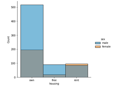
Before applying the algorithms, the data sets are pre-processed. The categorical values are converted into numerical values and statistical information of each data set is gathered. The distribution of data for German, Adult and Heart datasets is shown in the below Figure 1.
The skewness observed from German datasets are represented in the Figure 2.
(a) Distribution of Age w.r.to Credit Risk
(b) Distribution of Job w.r.to Gender
(c) Distribution of Gender w.r.to Credit Risk
(d) Distribution of Housing w.r.to Gender Factor
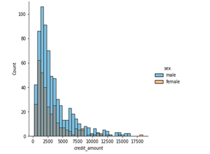
(e) Distribution of Credit Amount w.r.to Genderess
Figure 1. Distribution of attributes
(a) Skewness observed in Age distribution
(b) Skewness observed in Credit amount
Figure 2. Skewness observed from German Dataset
(a) Skewness observed in Age distribution
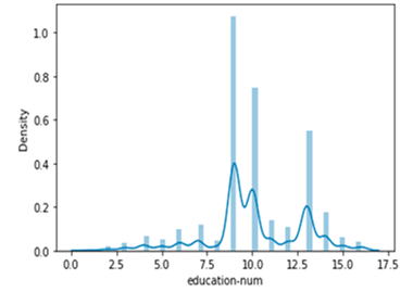
(b) Skewness observed in Educated People
Figure 3. Skewness observed from Adult Dataset
The skewness observed from adult datasets are represented in the Figure 3.
The skewness observed from Heart datasets are represented in the Figure 4.
(a) Skewness observed in Age distribution
(b) Skewness observed in Heart Risk Factor
Figure 4. Skewness observed from Heart Dataset
Table 1. Pre-training bias metrics of adult, heart disease and German datasets
|
Dataset |
Metric |
Features |
||||
|
F1(age) |
F2 |
F3 |
F4(risk) |
F5 |
||
|
Adult |
skewness |
1.02 |
1.94 |
-0.87 |
-0.37 |
0.1 |
|
CI |
2:7 |
1:3 |
1:22 |
3:7 |
2:133 |
|
|
KS |
> |
< |
> |
> |
< |
|
|
KL |
1.06 |
2.45 |
3.56 |
2.89 |
1.02 |
|
|
Disparity |
-0.324 |
-0.287 |
-0.21 |
-0.489 |
1.02 |
|
|
Heart disease |
skewness |
0.55 |
1.44 |
-0.31 |
0.22 |
0.089 |
|
CI |
1:25 |
3:26 |
2:51 |
1:82 |
1:28 |
|
|
KS |
> |
< |
> |
> |
< |
|
|
KL |
1.32 |
3.46 |
2.95 |
3.42 |
1.12 |
|
|
Disparity |
-0.4 |
-0.367 |
-0.23 |
-0.524 |
1.1 |
|
|
German dataset |
Skewness |
-0.145 |
0.493 |
-1.063 |
-1.23 |
-1.058 |
|
CI |
1:10 |
2:21 |
1:66 |
1:121 |
3:129 |
|
|
KS |
> |
< |
> |
> |
< |
|
|
KL |
1.45 |
4.561 |
2.45 |
4.56 |
1.23 |
|
|
Disparity |
-0.235 |
-0.41 |
-0.34 |
-0.46 |
-0.01 |
|
The metrics are tabulated for each feature from F1 to F5, the metrics such as skewness, CI, KS, KL and Disparity are considered and evaluated for the protected features of the Adult, Heat disease and also German datasets and are tabulated as shown in the Table 1. The Pre-training bias metrics of data sets is as above.
The model is evaluated using the traditional machine learning algorithms to test the performance of model before mitigating bias and after the mitigating the bias. The metrics used for measuring the performance are FP, FN and AUC. The FP rate is measured using the formula is as follows:
False Positive Rate = False Positives / (False Positives + True Negatives) (7)
The results are tabulated in the Table 2.
Table 2. Comparative analysis of datasets before and after mitigating bias
|
Dataset |
Before Mitigating Bias |
After Mitigating Bias |
||||
|
FP |
FN |
AUC |
FP |
FN |
AUC |
|
|
Adult |
73.12 |
35.2 |
7.6 |
51.4 |
31.45 |
4.54 |
|
Heart disease |
65.34 |
28.56 |
6.42 |
38.56 |
20.1 |
3.48 |
|
German dataset |
55.46 |
26.58 |
5.84 |
29.45 |
15.56 |
3.53 |
The below Figure 5 shows the ROC curve with biased data. The figure clearly shows that Black race has highest accuracy rate.
Figure 5. ROC curve for group wised biased data
After mitigating bias the ROC curve shows the reduced variance between the race and gender as shown in Figure 6.
Figure 6. ROC curve with mitigated bias in the data
In this paper, we have proposed algorithm to detect the bias from the given datasets, and mitigate the bias. The consequences of this work shows that not only bias in a model can be decreased without forfeiting model performance rate, but improving the performance. The various pre-training metrics used in the work are class imbalance, KL divergence, sample disparity and KS. Each metric is given weightage and the features are detected based on the maximum weightage. The model is trained to learn the unbiased data and show the significant improvement of the performance. ROC curve, False Positive Rate and False Negative Rate are used for bias trade-off. FPR and FNR are compared before mitigating bias and after mitigating bias and it is significantly decreased.
[1] Morstatter, F. (2016). Detecting and mitigating bias in social media. In 2016 IEEE/ACM International Conference on Advances in Social Networks Analysis and Mining (ASONAM), pp. 1347-1348. http://dx.doi.org/10.1109/ASONAM.2016.7752412
[2] Venugopalan, S., Narayanaswamy, A., Yang, S., Geraschenko, A., Lipnick, S., Makhortova, N., Hawrot, J., Marques, C., Pereira, J., Brenner, M., Rubin, L., Wainger, B., Berndl, M. (2019). It's easy to fool yourself: Case studies on identifying bias and confounding in bio-medical datasets. arXiv:1912.07661.
[3] Krishnan, S., Patel, J., Franklin, M.J., Goldberg, K. (2014). A methodology for learning, analyzing, and mitigating social influence bias in recommender systems. In Proceedings of the 8th ACM Conference on Recommender Systems, pp. 137-144. http://dx.doi.org/10.1145/2645710.2645740
[4] Hinduja, S. (2019). Mitigating the bias in empathy detection. In 2019 8th International Conference on Affective Computing and Intelligent Interaction Workshops and Demos (ACIIW), pp. 60-64. http://dx.doi.org/10.1109/ACIIW.2019.8925035
[5] Houser, K.A. (2019). Can AI Solve the Diversity Problem in the Tech Industry? Mitigating Noise and Bias in Employment Decision-Making. By permission of the Board of Trustees of the Leland Stanford Junior University, from the Stanford Technology Law Review at 22 STA, Available at SSRN: https://ssrn.com/abstract=3344751
[6] Wachinger, C., Becker, B.G., Rieckmann, A., Pölsterl, S. (2019). Quantifying confounding bias in neuroimaging datasets with causal inference. In International Conference on Medical Image Computing and Computer-Assisted Intervention, pp. 484-492. http://dx.doi.org/10.1007/978-3-030-32251-9_53
[7] Procopio, M., Mosca, A., Scheidegger, C.E., Wu, E., Chang, R. (2021). Impact of cognitive biases on progressive visualization. IEEE Transactions on Visualization and Computer Graphics. http://dx.doi.org/10.1109/TVCG.2021.3051013
[8] Khalil, A., Ahmed, S.G., Khattak, A.M., Al-Qirim, N. (2020). Investigating bias in facial analysis systems: A systematic review. IEEE Access, 8: 130751-130761. http://doi.org/10.1109/ACCESS.2020.3006051
[9] Dixon, L., Li, J., Sorensen, J., Thain, N., Vasserman, L. (2018). Measuring and mitigating unintended bias in text classification. In Proceedings of the 2018 AAAI/ACM Conference on AI, Ethics, and Society, pp. 67-73. https://doi.org/10.1145/3278721.3278729
[10] Edizel, B., Bonchi, F., Hajian, S., Panisson, A., Tassa, T. (2020). FaiRecSys: Mitigating algorithmic bias in recommender systems. International Journal of Data Science and Analytics, 9(2): 197-213. http://dx.doi.org/10.1007/s41060-019-00181-5
[11] Dixon, M.F., Halperin, I., Bilokon, P. (2020). Machine Learning in Finance. Springer International Publishing. https://doi.org/10.1007/978-3-030-41068-1
[12] https://archive.ics.uci.edu/ml/machine-learning-databases/adult/, accessed on 10/10/2021.
[13] https://archive.ics.uci.edu/ml/datasets/statlog+(german+credit+data), accessed on 10/10/2021.