Erick P. Herrera-Granda* | Leandro L. Lorente-Leyva | Jenny Yambay | Jesús Aranguren | Marcelo Ibarra | Julio Peña
© 2022 IIETA. This article is published by IIETA and is licensed under the CC BY 4.0 license (http://creativecommons.org/licenses/by/4.0/).
OPEN ACCESS
Dynamic modeling and control are research fields that hake kept the attention of researchers over the last decades. In this paper we describe a detailed approach to model, design and simulate a feedback controller for a quadrotor with the aim of giving the reader a detailed procedure to obtain the dynamic model and link this model with a controller design strategy. For this purpose, the dynamic model of the Parrot AR. Drone 2.0 was obtained using the Newton-Euler formulations. Next, the model was converted to the state space, and it was linearized to get the equations to perform a controller gain estimation process. Finally, the performance of state feedback controller visualized for both the linear and nonlinear models. Results shown that, the challenging goal of stabilizing the quadrotor at a desired trajectory, in short time without overshoot problems, can be achieved by means of a simple control strategy.
space states, controller modeling, quadrotor, trajectory tracking
Nowadays, unmanned aerial vehicles (UAVs) have gained an important space, as they can perform an autonomous track of pre-programmed routes. This allows performing complex aerial exploration tasks, transport of objects that represent a high risk for the crew and reconnaissance [1]. The box is a UAV consisting of four rotors located at the ends of a cruciform structure. A quadrotor is a UAV consisting of four rotors located at the ends of a cruciform structure that have become very popular in the recent years, due to its simplicity and easiness of use even when performing challenging tasks.
The quadrotor has been studied in a timely manner by the scientific community. As they are easy to control compared to other UAVs and their ability to perform complex maneuvers [2], for their ability to navigate autonomously in structured and unstructured environments [3, 4]; for their ability to perform cooperative tasks and proper transportation of objects [5]. Also, in the detection and tracking of human targets in real time [6]. The most important advantages of the quadrotor are stationary flights, vertical takeoff, and landing, which allows them to be used in densely populated environments. However, a disadvantage of this type of UAV is its flight time since they cannot perform long duration flight.
The AR. Drone 2.0 is a quadrotor manufactured by the French company Parrot. It has been selected as an experimental platform by several researchers due to the large number of sensors it carries and its low cost. However, because it has an internal controller to stabilize it, it is not possible to use the generic dynamic model to model its controller [7]. In the literature, it is possible to find works related to the modeling and control of these quadrotors [8]. Hernandez et al. [9] present a method to identify the modeling of the AR. Drone, they also propose a path tracing strategy to control its position. Bristeau et al. [10] show the architecture of the quadrotor. However, the values of its parameters are not disclosed.
In quadrotor research it is common to use filters and observers, because of the noise present in the sensor measurements and in some cases, it is not possible to compute all the states of the system [11-13]. Mokhtari et al. [14] present a feedback linearization and a linear observer for the control of a quadrotor. Wang and Shirinzadeh [15] use nonlinear observers to estimate the uncertainties and velocities of a framer knowing its position [16]. For the case of the AR. Drone, Santana et al. [17] use a Kalman filter to determine the system states based on the combination of inertial and visual data.
In the present research, the main contribution is the detailed description of a useful method, to perform modelling, simulation, and state feedback controller gain estimation of a quadcopter, by reducing the system to a linear simplification at the equilibrium point, to estimate the controller parameters that are used to control the real nonlinear model. As a first step, a complete dynamic model of the AR.Drone is proposed, which is obtained from the combination of the dynamic model of a generic quadrotor helicopter and the modeling of the internal controller of the AR. Drone. Then, the model is converted to the state space, and linearized at the equilibrium point. Next, the state feedback controller gains are calculated. Finally, the obtained gains are tested and simulated on both the linear and nonlinear model.
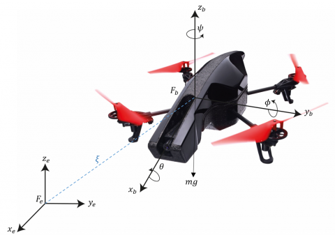
If a motion of the quadrotor in a three-dimensional space is considered, in which a fixed inertial frame of the earth Fe and to a body frame attached to the quadrotor Fb are established, as shown in Figure 1 [18, 19].
Figure 1. Quadricopter coordinate system
The position of the quadrotor center of mass would be at coordinates $\xi=[x, y, z]^{T}$ and that its orientation is given by the Euler angles yaw, roll and pitch $\eta=[\psi, \theta, \phi]^{T}$ and thus the dynamic equations of the quadrotor are [20]:
$m \ddot{\xi}=m g \boldsymbol{D}+\boldsymbol{R} F$ (1)
$I \dot{\Omega}=-\Omega \times I \Omega+\tau$ (2)
where, $\boldsymbol{D}=[0,0,-1]^{T}, \boldsymbol{R} \in S O(3)$ is the rotation matrix of the quadrotor Fb with respect to ground Fe, furthermore the vector of forces applied on the quadrotor is $F=[0,0, u]^{T}$ where u is the main thrust generated by the drone on the ground to propel itself. The total mass of the quadrotor is denoted as m and g is the gravitational acceleration. The variable $\Omega=[r, q, p]^{T}$ represents the vector that contains angular velocities of the drone, l represents the moment of inertia and $\tau$ is the total torque. Taking the functions $\sin (*)$ and $\cos (*)$ as $S *$ and $C *$ respectively, the rotation matrix is:
$R=\left(\begin{array}{ccc}C \theta C \phi & S \phi S \theta C \psi-C \phi S \psi & C \phi S \theta C \psi+S \phi S \psi \\ C \theta S \psi & S \phi S \theta S \psi+C \phi C \psi & C \phi S \theta S \psi-S \phi C \psi \\ -S \theta & S \phi C \theta & C \phi C \theta\end{array}\right)$
Moreover, an additional vector $\tilde{\tau}=\left[\tilde{\tau}_{\psi}, \tilde{\tau}_{\theta}, \tilde{\tau}_{\phi}\right]^{T}$ can be defined representing the generalized torque in the roll, pitch and yaw directions. Defined by the following expression:
$\tilde{\tau}=I^{-1} W^{-1}(-I \dot{W} \dot{\eta}-W \dot{\eta} \times I W \dot{\eta}+\tau)$ (3)
where the equivalence between the angular velocities with respect to the coordinate system and in the mobile reference system in the drone is:
$\Omega=W \dot{\eta}$
And the transformation matrix W as defined as:
$W=\left(\begin{array}{ccc}-\sin \theta & 0 & 1 \\ \cos \theta \sin \phi & \cos \phi & 0 \\ \cos \theta \cos \phi & -\sin \phi & 0\end{array}\right)$
By substituting the dynamic equilibrium equations of forces and torques, and their respective clearance, the dynamic model of the quadrotor can be reduced by the following equations:
$\ddot{x}=\frac{u}{m}(\cos \psi \sin \theta \cos \phi+\sin \psi \sin \phi)$ (4)
$\ddot{y}=\frac{u}{m}(\sin \psi \sin \theta \cos \phi-\cos \psi \sin \phi)$ (5)
$\ddot{z}=\frac{u}{m}(\cos \theta \cos \phi)-g$ (6)
$\ddot{\psi}=\tilde{\tau}_{\psi}$ (7)
$\ddot{\theta}=\tilde{\tau}_{\theta}$ (8)
$\ddot{\phi}=\tilde{\tau}_{\phi}$ (9)
where the principal thrust and angular moments $\tilde{\tau}_{\psi}, \tilde{\tau}_{\theta}, \tilde{\tau}_{\phi}$, s are the control inputs. In order to model an internal controller on board the drone, Eqns. (10) to (13) which relate to the vertical acceleration and angular accelerations, can be proposed with the inputs of the control system:
$\ddot{z}=-a_{1} \dot{z}+a_{3} u_{z}$ (10)
$\ddot{\phi}=-b_{1} \dot{\phi}-b_{2} \phi+b_{3} u_{\phi}$ (11)
$\ddot{\theta}=-c_{1} \dot{\theta}-c_{2} \theta+c_{3} u_{\theta}$ (12)
$\ddot{\psi}=-b_{1} \dot{\psi}-b_{2} \psi+b_{3} u_{\psi}$ (13)
$\dot{x}_{3}=x_{4}$ (14)
$\dot{x}_{4}=\left(\frac{-\cos \left(x_{11}\right) \sin \left(x_{7}\right)+\sin \left(x_{11}\right) \sin \left(x_{9}\right) \cos \left(x_{7}\right)}{m}\right) U(1)$ (15)
$\dot{x}_{5}=x_{6}$
$\dot{x}_{6}=-g+\left(\frac{\cos \left(x_{9}\right) \cos \left(x_{7}\right)}{m} \quad\right) U(1)$ (16)
$\dot{x}_{7}=x_{8}$
$\dot{x}_{8}=\frac{I_{y y}-I_{z z}}{I_{x x}} x_{10} x_{12}-\frac{J_{t p}}{I_{x x}} x_{8} \omega+\frac{U(2)}{I_{x x}}$ (17)
$\dot{x}_{9}=x_{10}$
$\dot{x}_{10}=\frac{I_{z z}-I_{x x}}{I_{y y}} x_{8} x_{12}-\frac{J_{t p}}{I_{y y}} x_{8} \omega+\frac{U(3)}{I_{x x}}$ (18)
$\dot{x}_{11}=x_{12}$
$\dot{x}_{12}=\frac{I_{x x}-I_{y y}}{I_{z z}} x_{8} x_{10}+\frac{U(4)}{I_{z z}}$ (19)
2.1 Modeling of the control system
As can be noticed in the state equations proposed above, the flight control system is nonlinear and has special complexity due to the presence of the trigonometric functions sine and cosine. Therefore, the proposed controller developed consists of a feedback controller whose control laws will be obtained by means of an equivalent controller linearized only at an equilibrium point.
To obtain the equilibrium point the first thing that was done is to equalize the derivatives of each state to zero where the equilibrium point of the system is obtained so that the equations are:
$0=x_{2}$
$\mathrm{x} 0=\left(\frac{\sin \left(x_{11}\right) \sin \left(x_{7}\right)+\cos \left(x_{11}\right) \sin \left(x_{9}\right) \cos \left(x_{7}\right)}{m} \quad\right) U(1)_{Q}$ (20)
$0=x_{4}$
$0=\left(\frac{-\cos \left(x_{11}\right) \sin \left(x_{7}\right)+\sin \left(x_{11}\right) \sin \left(x_{9}\right) \cos \left(x_{7}\right)}{m} \quad\right) U(1)_{Q}$ (21)
$0=x_{6}$
$\mathrm{x} 0=-g+\left(\frac{\cos \left(x_{9}\right) \cos \left(x_{7}\right)}{m}\right) U(1)_{Q}$ (22)
$0=x_{8}$
$0=\frac{l_{y y}-l_{z z}}{l_{x x}} x_{10} x_{12}-\frac{J_{t p}}{l_{x x}} x_{10} \omega+\frac{U(2)_{Q}}{l_{x x}}$ (23)
$0=x_{10}$
$0=\frac{l_{z z}-l_{x x}}{l_{y y}} x_{8} x_{12}-\frac{J_{t p}}{l_{y y}} x_{8} \omega+\frac{U(3)_{Q}}{l_{x x}}$ (24)
$0=x_{12}$
$0=\frac{l_{x x}-l_{y y}}{l_{z z}} x_{8} x_{10}+\frac{U(4)_{Q}}{l_{z z}}$ (25)
To obtain the equilibrium point we equated the derivatives of each state xi to zero where we have the equilibrium point of the system xQ, for the corresponding equilibrium inputs $U(1)_{Q}, U(2)_{Q}, U(3)_{Q}$ and $U(4)_{Q}$, thus replacing and simplifying Eqns. (14) to (25) we obtain:
$0=x_{2}$
$0=\sin \left(x_{11}\right) \sin \left(x_{7}\right)+\cos \left(x_{11}\right) \sin \left(x_{9}\right) \cos \left(x_{7}\right)$ (26)
$\begin{aligned} 0 &=x_{4} \\ 0=-\cos \left(x_{11}\right) \sin \left(x_{2}\right) &+\sin \left(x_{11}\right) \sin \left(x_{9}\right) \cos \left(x_{7}\right) \end{aligned}$ (27)
$0=x_{6}$
$0=-g+\left(\frac{\cos \left(x_{9}\right) \cos \left(x_{7}\right)}{m}\right) U(1)_{Q}$
$0=x_{8}$
$0=\frac{U(2)_{Q}}{l_{x x}}$
$0=x_{10}$
By subtracting $\sin \left(x_{9}\right) \cos \left(x_{7}\right)$ from (26) and replacing in (27) we have the value of x7 at the equilibrium point:
$\sin \left(x_{9}\right) \cos \left(x_{7}\right)=\frac{\cos \left(x_{11}\right) \sin \left(x_{7}\right)}{\sin \left(x_{11}\right)}$
$0=\sin \left(x_{11}\right) \sin \left(x_{7}\right)+\cos \left(x_{11}\right) \frac{\cos \left(x_{11}\right) \sin \left(x_{7}\right)}{\sin \left(x_{11}\right)}$
$0=\sin ^{2}\left(x_{11}\right) \sin \left(x_{7}\right)+\cos ^{2}\left(x_{11}\right) \sin \left(x_{7}\right)$
$0=\sin \left(x_{7}\right)\left(\sin ^{2}\left(x_{11}\right)+\cos ^{2}\left(x_{11}\right)\right)$
$0=\sin \left(x_{7}\right)$
$x_{7}=k \pi$
Replacing this value in (27) gives $0=\operatorname{sen}\left(x_{11}\right) \operatorname{sen}\left(x_{9}\right)$, so $x_{9}, x_{11}=k \pi$. Finally, the equilibrium point for the twelve state variables of the system is $x_{Q}=[X, 0, Y, 0, Z, 0, k \pi, 0, k \pi, 0, k \pi, 0]^{T}$.
For the linearization of the system, we proceed to obtain the matrices A B C D of a system of equivalent behavior at the equilibrium point, so the matrices for the linearized system are obtained as:
The system in state space:
$\dot{x}=A x+B u$
$\dot{y}=C x+D u$
It is equivalent at the break-even point with:
$\Delta \dot{x}=\bar{A} \Delta x+\bar{B} u$
$\Delta \dot{y}=\bar{C} \Delta x+\bar{D} u$
where:
$\bar{A}={{\left. \frac{\partial F}{\partial x} \right|}_{\begin{matrix} {{x}_{Q}} \\{{u}_{Q}} \\\end{matrix}}}$
$\bar{B}={{\left. \frac{\partial F}{\partial u} \right|}_{\begin{matrix} {{x}_{Q}} \\{{u}_{Q}} \\\end{matrix}}}$
$\bar{C}={{\left. \frac{\partial G}{\partial x} \right|}_{\begin{matrix} {{x}_{Q}} \\{{u}_{Q}} \\\end{matrix}}}$
$\bar{D}={{\left. \frac{\partial G}{\partial u} \right|}_{\begin{matrix} {{x}_{Q}} \\{{u}_{Q}} \\\end{matrix}}}$
Then the value of the equivalent state matrix of the linearized system is determined by obtaining the partial derivatives of each equation of states with respect to each of the states:
$\bar{A}={{\left. \frac{\partial F}{\partial x} \right|}_{\begin{matrix} {{x}_{Q}} \\{{u}_{Q}} \\\end{matrix}}}=\left[\begin{array}{cccc}\frac{\partial F_{1}}{\partial x_{1}} & \frac{\partial F_{1}}{\partial x_{2}} & \cdots & \frac{\partial F_{1}}{\partial x_{n}} \\ \frac{\partial F_{2}}{\partial x_{1}} & \frac{\partial F_{2}}{\partial x_{2}} & \cdots & \frac{\partial F_{2}}{\partial x_{n}} \\ \vdots & \vdots & \ddots & \vdots \\ \frac{\partial F_{n}}{\partial x_{1}} & \frac{\partial F_{n}}{\partial x_{2}} & \cdots & \frac{\partial F_{n}}{\partial x_{n}}\end{array}\right]$
Performing this process for the twelve states we obtain the matrices A, B, C and D, which can be observed respectively in the linearized state space:
$\mathrm{A}=\left(\begin{array}{cccccccccccc}0 & 1 & 0 & 0 & 0 & 0 & 0 & 0 & 0 & 0 & 0 & 0 \\ 0 & 0 & 0 & 0 & 0 & 0 & 0 & 0 & \pm g & 0 & 0 & 0 \\ 0 & 0 & 0 & 1 & 0 & 0 & 0 & 0 & 0 & 0 & 0 & 0 \\ 0 & 0 & 0 & 0 & 0 & 0 & -g & 0 & 1 & 0 & 0 & 0 \\ 0 & 0 & 0 & 0 & 0 & 1 & 0 & 0 & 0 & 0 & 0 & 0 \\ 0 & 0 & 0 & 0 & 0 & 0 & 0 & 0 & 0 & 0 & 0 & 0 \\ 0 & 0 & 0 & 0 & 0 & 0 & 0 & 1 & 0 & 0 & 0 & 0 \\ 0 & 0 & 0 & 0 & 0 & 0 & 0 & 0 & 0 & -J t p * \frac{\omega}{l y y} & 0 & 0 \\ 0 & 0 & 0 & 0 & 0 & 0 & 0 & 0 & 0 & 1 & 0 & 0 \\ 0 & 0 & 0 & 0 & 0 & 0 & 0 & 0 & 0 & 0 & 0 & 0 \\ 0 & 0 & 0 & 0 & 0 & 0 & 0 & 0 & 0 & 0 & 0 & 1 \\ 0 & 0 & 0 & 0 & 0 & 0 & 0 & 0 & 0 & 0 & 0 & 0\end{array}\right)$
$\mathrm{B}=\left(\begin{array}{cccc}0 & 1 & 0 & 0 \\ 0 & 0 & 0 & 0 \\ 0 & 0 & 0 & 1 \\ 0 & 0 & 0 & 0 \\ 0 & 0 & 0 & 0 \\ 1 / m & 0 & 0 & 0 \\ 0 & 0 & 0 & 0 \\ 0 & 1 / l_{x x} & 0 & 0 \\ 0 & 0 & 0 & 0 \\ 0 & 0 & 1 / l_{y y} & 0 \\ 0 & 0 & 0 & 0 \\ 0 & 0 & 0 & 1 / l_{z z}\end{array}\right)$
$C=\left(\begin{array}{llllllllllll}1 & 0 & 0 & 0 & 0 & 0 & 0 & 0 & 0 & 0 & 0 & 0 \\ 0 & 0 & 0 & 0 & 0 & 0 & 0 & 0 & 0 & 0 & 0 & 0 \\ 0 & 0 & 1 & 0 & 0 & 0 & 0 & 0 & 0 & 0 & 0 & 0 \\ 0 & 0 & 0 & 0 & 0 & 0 & 0 & 0 & 0 & 0 & 0 & 0 \\ 0 & 0 & 0 & 0 & 1 & 0 & 0 & 0 & 0 & 0 & 0 & 0 \\ 0 & 0 & 0 & 0 & 0 & 0 & 0 & 0 & 0 & 0 & 0 & 0 \\ 0 & 0 & 0 & 0 & 0 & 0 & 0 & 0 & 0 & 0 & 0 & 0 \\ 0 & 0 & 0 & 0 & 0 & 0 & 0 & 0 & 0 & 0 & 0 & 0 \\ 0 & 0 & 0 & 0 & 0 & 0 & 0 & 0 & 0 & 0 & 0 & 0 \\ 0 & 0 & 0 & 0 & 0 & 0 & 0 & 0 & 0 & 0 & 0 & 0 \\ 0 & 0 & 0 & 0 & 0 & 0 & 0 & 0 & 0 & 0 & 0 & 0 \\ 0 & 0 & 0 & 0 & 0 & 0 & 0 & 0 & 0 & 0 & 0 & 0\end{array}\right) \quad D=\left(\begin{array}{llll}0 & 0 & 0 & 0 \\ 0 & 0 & 0 & 0 \\ 0 & 0 & 0 & 0 \\ 0 & 0 & 0 & 0 \\ 0 & 0 & 0 & 0 \\ 0 & 0 & 0 & 0 \\ 0 & 0 & 0 & 0 \\ 0 & 0 & 0 & 0 \\ 0 & 0 & 0 & 0 \\ 0 & 0 & 0 & 0 \\ 0 & 0 & 0 & 0 \\ 0 & 0 & 0 & 0\end{array}\right)$
Finally, the linearized equivalent state space is:
$\Delta \dot{x}=\left(\begin{array}{cccccccccccc}0 & 1 & 0 & 0 & 0 & 0 & 0 & 0 & 0 & 0 & 0 & 0 \\ 0 & 0 & 0 & 0 & 0 & 0 & 0 & 0 & \pm g & 0 & 0 & 0 \\ 0 & 0 & 0 & 1 & 0 & 0 & 0 & 0 & 0 & 0 & 0 & 0 \\ 0 & 0 & 0 & 0 & 0 & 0 & -g & 0 & 1 & 0 & 0 & 0 \\ 0 & 0 & 0 & 0 & 0 & 1 & 0 & 0 & 0 & 0 & 0 & 0 \\ 0 & 0 & 0 & 0 & 0 & 0 & 0 & 0 & 0 & 0 & 0 & 0 \\ 0 & 0 & 0 & 0 & 0 & 0 & 0 & 1 & 0 & 0 & 0 & 0 \\ 0 & 0 & 0 & 0 & 0 & 0 & 0 & 0 & 0 & -J t p * \omega / l y y & 0 & 0 \\ 0 & 0 & 0 & 0 & 0 & 0 & 0 & 0 & 0 & 1 & 0 & 0 \\ 0 & 0 & 0 & 0 & 0 & 0 & 0 & 0 & 0 & 0 & 0 & 0 \\ 0 & 0 & 0 & 0 & 0 & 0 & 0 & 0 & 0 & 0 & 0 & 1 \\ 0 & 0 & 0 & 0 & 0 & 0 & 0 & 0 & 0 & 0 & 0 & 0\end{array}\right) \Delta x+\left(\begin{array}{cccc}0 & 1 & 0 & 0 \\ 0 & 0 & 0 & 0 \\ 0 & 0 & 0 & 1 \\ 0 & 0 & 0 & 0 \\ 0 & 0 & 0 & 0 \\ 1 / m & 0 & 0 & 0 \\ 0 & 0 & 0 & 0 \\ 0 & 1 / l_{x x} & 0 & 0 \\ 0 & 0 & 0 & 0 \\ 0 & 0 & 1 / l_{y y} & 0 \\ 0 & 0 & 0 & 0 \\ 0 & 0 & 0 & 1 / l_{z z}\end{array}\right)\left(\begin{array}{c}U(1) \\ U(2) \\ U(3) \\ U(4)\end{array}\right)$ (28)
$\Delta \dot{y}=\left(\begin{array}{llllllllllll}1 & 0 & 0 & 0 & 0 & 0 & 0 & 0 & 0 & 0 & 0 & 0 \\ 0 & 0 & 0 & 0 & 0 & 0 & 0 & 0 & 0 & 0 & 0 & 0 \\ 0 & 0 & 1 & 0 & 0 & 0 & 0 & 0 & 0 & 0 & 0 & 0 \\ 0 & 0 & 0 & 0 & 0 & 0 & 0 & 0 & 0 & 0 & 0 & 0 \\ 0 & 0 & 0 & 0 & 1 & 0 & 0 & 0 & 0 & 0 & 0 & 0 \\ 0 & 0 & 0 & 0 & 0 & 0 & 0 & 0 & 0 & 0 & 0 & 0 \\ 0 & 0 & 0 & 0 & 0 & 0 & 0 & 0 & 0 & 0 & 0 & 0 \\ 0 & 0 & 0 & 0 & 0 & 0 & 0 & 0 & 0 & 0 & 0 & 0 \\ 0 & 0 & 0 & 0 & 0 & 0 & 0 & 0 & 0 & 0 & 0 & 0 \\ 0 & 0 & 0 & 0 & 0 & 0 & 0 & 0 & 0 & 0 & 0 & 0 \\ 0 & 0 & 0 & 0 & 0 & 0 & 0 & 0 & 0 & 0 & 0 & 0 \\ 0 & 0 & 0 & 0 & 0 & 0 & 0 & 0 & 0 & 0 & 0 & 0\end{array}\right) \Delta x+\left(\begin{array}{llll}0 & 0 & 0 & 0 \\ 0 & 0 & 0 & 0 \\ 0 & 0 & 0 & 0 \\ 0 & 0 & 0 & 0 \\ 0 & 0 & 0 & 0 \\ 0 & 0 & 0 & 0 \\ 0 & 0 & 0 & 0 \\ 0 & 0 & 0 & 0 \\ 0 & 0 & 0 & 0 \\ 0 & 0 & 0 & 0 \\ 0 & 0 & 0 & 0 \\ 0 & 0 & 0 & 0\end{array}\right)\left(\begin{array}{l}U(1) \\ U(2) \\ U(3) \\ U(4)\end{array}\right)$ (29)
Once the linearized equivalent system has been obtained, a linear feedback controller is applied, whose objective is to transform the state variable in the available input by means of a gain matrix k, as follows:
$u=-k x$
Then the proposed matrix presents twelve gains $k_{1}, k_{2}, k_{3}, \ldots, k_{12}$ that will allow to have control of the outputs from the desired inputs for the twelve states and were placed in the matrix from the effect that each input has on the respective states. So for example if it is known that if the input U(1) corresponds to vertical thrust, this will have an effect on the state variables x5 and x6 corresponding to the vertical position Z and its respective velocity $\dot{Z}$, the input U(2) corresponds to a momentum in roll so this will have an effect on the state variables x7 and x8 causing an angular displacement in roll $\theta$ and its respective angular velocity $\dot{\theta}$. Input U(3) corresponds to a momentum in pitch so this will have effect on state variables x9 and x10 causing an angular displacement in pitch $\emptyset$ and its respective angular velocity $\dot{\emptyset}$. Finally, the input U(4) corresponds to a moment in yaw, so this will have effect on the state variables x11 and x12 causing an angular displacement in pitch $\psi$ and its respective angular velocity $\dot{\psi}$. Then the proposed gain matrix is:
$k=\left(\begin{array}{cccccccccccc}0 & 0 & 0 & 0 & k_{5} & k_{6} & 0 & 0 & 0 & 0 & 0 & 0 \\ 0 & 0 & 0 & 0 & 0 & 0 & k_{7} & k_{8} & 0 & 0 & 0 & 0 \\ 0 & 0 & 0 & 0 & 0 & 0 & 0 & 0 & k_{9} & k_{10} & 0 & 0 \\ 0 & 0 & 0 & 0 & 0 & 0 & 0 & 0 & 0 & 0 & k_{11} & k_{12}\end{array}\right)$
So the controller is, for the values of the state variables xi at the desired stabilization point $x_{\mathrm{i} \delta}$ for $i=1,2,3, \ldots, 12$, is:
$u=-\left(\begin{array}{cccccccccccc}0 & 0 & 0 & 0 & k_{5} & k_{6} & 0 & 0 & 0 & 0 & 0 & 0 \\ 0 & 0 & 0 & 0 & 0 & 0 & k_{7} & k_{8} & 0 & 0 & 0 & 0 \\ 0 & 0 & 0 & 0 & 0 & 0 & 0 & 0 & k_{9} & k_{10} & 0 & 0 \\ 0 & 0 & 0 & 0 & 0 & 0 & 0 & 0 & 0 & 0 & k_{11} & k_{12}\end{array}\right) \left(\begin{array}{c} x_{1 \delta}\\ x_{2 \delta} \\ x_{3 \delta} \\ x_{4 \delta} \\ x_{5 \delta} \\ x_{6 \delta} \\ x_{7 \delta} \\ x_{8 \delta} \\ x_{9 \delta} \\ x_{10 \delta} \\ x_{11 \delta} \\ x_{12 \delta}\end{array}\right)=\left(\begin{array}{c}-k_{5} x_{5 \delta}-k_{6} x_{6 \delta} \\ -k_{7} x_{7 \delta}-k_{8} x_{8 \delta} \\ -k_{9} x_{9 \delta}-k_{10} x_{10 \delta} \\ -k_{11} x_{11 \delta}-k_{12} x_{12 \delta}\end{array}\right)$
Since the system to be controlled is $\dot{x}=A x+B u$, then by means of the input found as a function of gains it can be rewritten as:
$B u=\left(\begin{array}{cccc}0 & 1 & 0 & 0 \\ 0 & 0 & 0 & 0 \\ 0 & 0 & 0 & 1 \\ 0 & 0 & 0 & 0 \\ 0 & 0 & 0 & 0 \\ 1 / m & 0 & 0 & 0 \\ 0 & 0 & 0 & 0 \\ 0 & 1 / l_{x x} & 0 & 0 \\ 0 & 0 & 0 & 0 \\ 0 & 0 & 1 / l_{y y} & 0 \\ 0 & 0 & 0 & 0 \\ 0 & 0 & 0 & 1 / l_{z z}\end{array}\right) \left(\begin{array}{c}-k_{5} x_{5 \delta}-k_{6} x_{6 \delta} \\ -k_{7} x_{7 \delta}-k_{8} x_{8 \delta} \\ -k_{9} x_{9 \delta}-k_{10} x_{10 \delta} \\ -k_{11} x_{11 \delta}-k_{12} x_{12 \delta}\end{array}\right) =\left(\begin{array}{c}0 \\ 0 \\ 0 \\ 0 \\ 0 \\ \frac{-k_{5} x_{5 \delta}-k_{6} x_{6 \delta}}{m} \\ 0 \\ \frac{-k_{7} x_{7 \delta}-k_{8} x_{8 \delta}}{l_{x x}} \\ 0 \\ \frac{-k_{9} x_{9 \delta}-k_{10} x_{10 \delta}}{l_{y y}} \\ 0 \\ \frac{ -k_{11} x_{11 \delta}-k_{12} x_{12 \delta}}{ l_{z z}}\end{array}\right)$
Finally, by summing the matrices $A x_{\delta}+B u$, the following is obtained:
$\dot{x}=\left(\begin{array}{cccccccccccc}0 & 1 & 0 & 0 & 0 & 0 & 0 & 0 & 0 & 0 & 0 & 0 \\ 0 & 0 & 0 & 0 & 0 & 0 & 0 & 0 & g & 0 & 0 & 0 \\ 0 & 0 & 0 & 1 & 0 & 0 & 0 & 0 & 0 & 0 & 0 & 0 \\ 0 & 0 & 0 & 0 & 0 & 0 & -g & 0 & 0 & 0 & 0 & 0 \\ 0 & 0 & 0 & 0 & 0 & 1 & 0 & 0 & 0 & 0 & 0 & 0 \\ 0 & 0 & 0 & 0 & -k_{5} / m & -k_{6} / m & 0 & 0 & 0 & 0 & 0 & 0 \\ 0 & 0 & 0 & 0 & 0 & 0 & 0 & 1 & 0 & 0 & 0 & 0 \\ 0 & 0 & 0 & 0 & 0 & 0 & -k_{7} / l_{x x} & -k_{8} / l_{x x} & 0 & -J_{t p} / l_{x x} & 0 & 0 \\ 0 & 0 & 0 & 0 & 0 & 0 & 0 & 0 & 0 & 1 & 0 & 0 \\ 0 & 0 & 0 & 0 & 0 & 0 & 0 & w & -k_{9} / l_{y y} & -k_{10} / l_{y y} & 0 & 0 \\ 0 & 0 & 0 & 0 & 0 & 0 & 0 & 0 & 0 & 0 & 0 & 1 \\ 0 & 0 & 0 & 0 & 0 & 0 & 0 & 0 & 0 & 0 & -k_{11} / l z z & -k_{12} / l z z\end{array}\right) \left(\begin{array}{c} x_{1 \delta}\\ x_{2 \delta} \\ x_{3 \delta} \\ x_{4 \delta} \\ x_{5 \delta} \\ x_{6 \delta} \\ x_{7 \delta} \\ x_{8 \delta} \\ x_{9 \delta} \\ x_{10 \delta} \\ x_{11 \delta} \\ x_{12 \delta}\end{array}\right)$
Furthermore, if we limit the range of rotation about the axes between $-\pi<\emptyset<\pi$ then $\pm g=g$ and applying the equilibrium point the matrix A the final system is:
$A=\left(\begin{array}{cccccccccccc}0 & 1 & 0 & 0 & 0 & 0 & 0 & 0 & 0 & 0 & 0 & 0 \\ 0 & 0 & 0 & 0 & 0 & 0 & 0 & 0 & g & 0 & 0 & 0 \\ 0 & 0 & 0 & 1 & 0 & 0 & 0 & 0 & 0 & 0 & 0 & 0 \\ 0 & 0 & 0 & 0 & 0 & 0 & -g & 0 & 0 & 0 & 0 & 0 \\ 0 & 0 & 0 & 0 & 0 & 1 & 0 & 0 & 0 & 0 & 0 & 0 \\ 0 & 0 & 0 & 0 & -k_{5} / m & -k_{6} / m & 0 & 0 & 0 & 0 & 0 & 0 \\ 0 & 0 & 0 & 0 & 0 & 0 & 0 & 1 & 0 & 0 & 0 & 0 \\ 0 & 0 & 0 & 0 & 0 & 0 & -k_{7} / l_{x x} & -k_{8} / l_{x x} & 0 & -J_{t p} / l_{x x} & 0 & 0 \\ 0 & 0 & 0 & 0 & 0 & 0 & 0 & 0 & 0 & 1 & 0 & 0 \\ 0 & 0 & 0 & 0 & 0 & 0 & 0 & w & -k_{9} / l_{y y} & -k_{10} / l_{y y} & 0 & 0 \\ 0 & 0 & 0 & 0 & 0 & 0 & 0 & 0 & 0 & 0 & 0 & 1 \\ 0 & 0 & 0 & 0 & 0 & 0 & 0 & 0 & 0 & 0 & -k_{11} / l z z & -k_{12} / l z z\end{array}\right)$
where, A is an element of great importance for the analysis due to the fact that by finding the eigenvalues of the matrix the characteristic polynomial can be found, which when equated to the poles located in the appropriate geometric location will allow a control action. The eigenvalues and the characteristic polynomial are obtained as shown in the following equation:
$(s+a)^{12}=|S I-A|$ (30)
where, (s+a)12 represents the location of the poles of the new stable and controlled system, which will be located in the position s=-a, which is appropriate since in this way it is a stable system since the poles are all located in the negative half-plane for x, where as a has a higher value stability will be reached in less time, and |SI-A| is the method by which the characteristic polynomial of the system is obtained.
By making the poles of the controlled system equal to the poles of the characteristic polynomial the system is controlled by the gains $k_{1}, k_{2}, k_{3}, \ldots, k_{12}$.
Developing the left-hand side of the equation we have the polynomial:
$\begin{aligned}(s+a)^{12}=s^{12} &+12 a s^{11}+66 a^{2} s^{10}+220 a^{3} s^{9}+220 a^{3} s^{9} \\ &+495 a^{4} s^{8}+792 a^{5} s^{7}+924 a^{6} s^{6}+792 a^{7} s^{5} \\ &+495 a^{8} s^{4}+220 a^{9} s^{3}+66 a^{10} s^{2}+12 a^{11} s \\ &+a^{12} \end{aligned}$
Given the complexity of the system and the equations involved, a code was developed in Matlab software to obtain the characteristic polynomial. Then, from the coefficients of each degree of the equation, eight equations are generated to calculate the eight gains.
By executing the eight equations of the controller were obtained, since although the equations are of degree 12 the elements of degree $s^{0}, s^{1}, s^{2}, s^{3}$, and $s^{4}$ do not have coefficients. Being the following equations:
$e q 1=(k 5 * k 7 * k 9 * k 11) /\left(I_{x x} * I_{y y} * I_{z z} * m\right)=495 * a ^{\wedge} 8$
$\begin{aligned} e q 2=(k 5 * k 7 *& k 9 * k 12+k 5 * k 7 * k 10 * k 11+k 5 * k 8 * k 9 \\ * &k 11+k 6 * k 7 * k 9 * k 11) \\ & /\left(I_{x x} * I_{y y} * I_{z z} * m\right)==792 * a^{\wedge} 7\end{aligned}$
$e q 3=(k 5 * k 7 * k 10 * k 12+k 5 * k 8 * k 9 * k 12+k 5 * k 8 * k 10 * k 11+k 6 * k 7 * k 9 * k 12+k 6 * k 7 * k 10 * k 11+k 6 * k 8 * k 9 * k 11$
$\left.+k 7 * k 9 * k 11 * m+I_{x x} * k 5 * k 9 * k 11+I_{y y} * k 5 * k 7 * k 11+I_{z z} * k 5 * k 7 * k 9+I_{y y} * J_{t p} * k 5 * k 11 * w\right)$
$/\left(I_{x x} * I_{y y} * I_{z z} * m\right)==924 * a^{\wedge}6$
$\begin{aligned} e q 4=(k 5 * k 8 *& k 10 * k 12+k 6 * k 7 * k 10 * k 12+k 6 * k 8 * k 9 * k 12+k 7 * k 9 * k 12 * m+k 8 * k 9 * k 11 * m+I_{x x} * k 5 * k 9 * k 12 \\ &+I_{x x} * k 5 * k 10 * k 11+I_{x x} * k 6 * k 9 * k 11+I_{y y} * k 5 * k 7 * k 12+I_{y y} * k 5 * k 8 * k 11+I_{y y} * k 6 * k 7 * k 11+I_{z z} \\ &\left.* k 5 * k 7 * k 10+I_{z z} * k 5 * k 8 * k 9+I_{z z} * k 6 * k 7 * k 9+I_{y y} * J_{t p} * k 5 * k 12 * w+I_{y y} * J_{t p} * k 6 * k 11 * w\right) \\ & /\left(I_{x x} * I_{y y} * I_{z z} * m\right)==792 * a^{\wedge}5\end{aligned}$
$\begin{aligned} e q 5=(k 6 * k 8& * k 10 * k 12+k 7 * k 10 * k 12 * m+k 8 * k 9 * k 12 * m+k 8 * k 10 * k 11 * m+I_{x x} * I_{y y} * k 5 * k 11+I_{x x} * I_{z z} * k 5 \\ & * k 9+I_{y y} * I_{z z} * k 5 * k 7+I_{x x} * k 5 * k 10 * k 12+I_{x x} * k 6 * k 9 * k 12+I_{x x} * k 6 * k 10 * k 11+I_{y y} * k 5 * k 8 * k 12 \\ &+I_{y y} * k 6 * k 7 * k 12+I_{y y} * k 6 * k 8 * k 11+I_{z z} * k 5 * k 8 * k 10+I_{z z} * k 6 * k 7 * k 10+I_{z z} * k 6 * k 8 * k 9+I_{x x} * k 9 \\ & * k 11 * m+I_{y y} * k 7 * k 11 * m+I_{z z} * k 7 * k 9 * m+I_{y y} * I_{z z} * J_{t p} * k 5 * w+I_{y y} * J_{t p} * k 6 * k 12 * w+I_{y y} * J_{t p} * k 11 \\ & * m *\left(/\left(I_{x x} * I_{y y} * I_{z z} * m\right)==495 * a^{\wedge}4\right.\end{aligned}$
$\begin{aligned} e q 6=(k 8 * k 10& * k 12 * m+I_{x x} * I_{y y} * k 5 * k 12+I_{x x} * I_{y y} * k 6 * k 11+I_{x x} * I_{z z} * k 5 * k 10+I_{x x} * I_{z z} * k 6 * k 9+I_{y y} * I_{z z} * k 5 * k 8 \\ &+I_{y y} * I_{z z} * k 6 * k 7+I_{x x} * k 6 * k 10 * k 12+I_{y y} * k 6 * k 8 * k 12+I_{z z} * k 6 * k 8 * k 10+I_{x x} * k 9 * k 12 * m+I_{x x} \\ & * k 10 * k 11 * m+I_{y y} * k 7 * k 12 * m+I_{y y} * k 8 * k 11 * m+I_{z z} * k 7 * k 10 * m+I_{z z} * k 8 * k 9 * m+I_{y y} * I_{z z} * J_{t p} \\ &\left.* k 6 * w+I_{y y} * J_{t p} * k 12 * m * w\right) /\left(I_{x x} * I_{y y} * I_{z z} * m\right)==220 * a^{\wedge} 3 \end{aligned}$
$\begin{aligned} e q 7=\left(I_{x x} * I_{y y} *\right.& I_{z z} * k 5+I_{x x} * I_{y y} * k 6 * k 12+I_{x x} * I_{z z} * k 6 * k 10+I_{x x} * I_{y y} * k 11 * m+I_{x x} * I_{z z} * k 9 * m+I_{y y} * I_{z z} * k 7 * m+I_{x x} \\ &\left.* k 10 * k 12 * m+I_{y y} * k 8 * k 12 * m+I_{z z} * k 8 * k 10 * m+I_{y y} * I_{z z} * J_{t p} * m * w\right) /\left(I_{x x} * I_{y y} * I_{z z} * m\right)==66 * a^{\wedge}2 \end{aligned}$
$e q 8=\left(I_{x x} * I_{y y} * I_{z z} * k 6+I_{x x} * I_{y y} * k 12 * m+I_{x x} * I_{z z} * k 10 * m+I_{y y} * I_{z z} * k 8 * m\right) /\left(I_{x x} * I_{y y} * I_{z z} * m\right)==12 * a$
Finally, MATLAB is asked to solve the system obtaining the exact value of the controller gains: $k_{5}=40.00289$, $k_{6}=12.051$, $k_{7}=30.30082$, $k_{8}=5.00023$, $k_{9}=30.30082$, $k_{10}=5.00023$, $k_{11}=30.30082$, $k_{12}=5.00023$.
Thus, the control laws are determined as follows:
$U(1)=\frac{m\left(g-k_{5}\left(x_{5}-Z_{d}\right)-k_{6} x_{6}\right.}{\cos \left(x_{9}\right) \cos \left(x_{7}\right)}$ (31)
$U(2)=-k_{7}\left(x_{7}-\theta_{d}\right)-k_{8} x_{8}$ (32)
$U(3)=-k_{9}\left(x_{9}-\emptyset_{d}\right)-k_{10} x_{10}$ (33)
$U(4)=-k_{11}\left(x_{11}-\psi_{d}\right)-k_{12} x_{12}$ (34)
The design of the linear and nonlinear controllers, whose mathematical equations were previously formulated, was developed in MATLAB where the calculation of the above gains is presented.
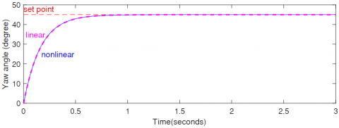
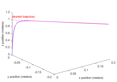
This section presents, an example of the results obtained through the flight simulations done in MATLAB, using the controller defined by Eqns. (31) to (34). The differential equation system of the model was solved using ode45 function using state space Eqns. (14) to (25) for the nonlinear model and the linear model was solved to get the simulations trough Eqns. (28) and (29), which let us compare how much the linearized system approximates in performance to the real nonlinear model. As a first example we took the input desired values: $z_{d}=1 m, \theta_{d}=45^{0}, \emptyset_{d}=45^{0}, \psi_{d}=45^{0}$, thus the simulation output is presented in Figures 2 to 8.
Results shown that the feedback controller works very well. Figures 4 and 8 show how the drone stabilizes at a height of 1 meter, while it turns 45º in yaw linearly and at the same it turns 45º in pitch then it keeps this orientation describing the trajectory shown in Figure 8, which was the desired trajectory. In addition, the correct operation of the controller is verified since the desired yaw angle of this example defined an inclination of 45 degrees which would orient the drone to ascend obliquely, but as a flight height of 1 meter was defined for the controller, the yaw angle only provides orientation keeping the same height through the whole trajectory.
Summarizing, in Figures 2 to 8 it can be seen that, linear and nonlinear models performed pretty similar. This occurs die to the fact that the desired trajectory used for this example is close enough to the equilibrium point, thus demonstrating that linearization process was successful, but when a trajectory far enough from the equilibrium point is chosen, trajectories of the linear and nonlinear models would differ considerably, but in both cases the desired trajectory must be achieved.
It must be mentioned that it is well known that some of the disadvantages that comes with the feedback linearization method, is its lack of robustness over parameter uncertainties, so the parameters considered for this model should maintain their values. As most of these parameters were geometric values, the model should perform safely, but some parameters as the weight or wind conditions must be considered for further implementations. Another simplification that must be considered is the simplification performed in Eqns. (26) and (27) which constraints the model to a range of operation of 0 to $\pi$ for the roll and pitch angles.
Figure 2. x-position of the quadrotor for the linear and nonlinear models
Figure 3. y-position of the quadrotor for the linear and nonlinear models
Figure 4. z-position of the quadrotor for the linear and nonlinear models
Figure 5. roll Angle for the linear and nonlinear models
Figure 6. pitch Angle the linear and nonlinear models
Figure 7. yaw Angle for the linear and nonlinear models
Figure 8. Flight simulation for the linear and nonlinear models
In this paper we described a detailed approach of the modelling and design of a state feedback controller for a Parrot AR. Drone 2.0, as well as its dynamic modeling process, with the aim of giving the reader a detailed procedure to obtain the kinematics and link this model with the controller design strategies. The state feedback controller was selected as a good example that achieved the goal of controlling the drone trajectories, however, any other control strategy (like LQR, Fuzzy, Neural, and so on) could be used, and a comparison should be performed as further work.
The results of both linear and nonlinear controllers are very similar, as the desired trajectory values are not far enough from the equilibrium point. If they are too far away, the linear model would fail.
Results show that by applying an input for vertical thrust and moments in roll, pitch and yaw a vertical displacement of the quadrotor occurs because of the action of the U(1) thrust, while moving in x and y axis, due to the moments U(2), U(3), and at the same time, a rotation on yaw is performed by the momentum U(4); which corresponds to the expected results for the dynamic model with control.
It can be mentioned that feedback controller performed well for this kind of drone, because the desired trajectory was achieved in a short time, without presenting overshoot or stabilization problems.
[1] Schacht-Rodriguez, R., Ortiz-Torres, G., Garcia-Beltran, C.D., Astorga-Zaragoza, C.M., Ponsart, J.C., Perez-Estrada, A.J. (2018). Design and development of a UAV experimental platform. IEEE Latin America Transactions, 16(5): 1320-1327. https://doi.org/10.1109/TLA.2018.8408423
[2] Mellinger, D., Michael, N., Kumar, V. (2012). Trajectory generation and control for precise aggressive maneuvers with quadrotors. The International Journal of Robotics Research, 31(5): 664-674. https://doi.org/10.1177/0278364911434
[3] Achtelik, M., Bachrach, A., He, R., Prentice, S., Roy, N. (2009). Stereo vision and laser odometry for autonomous helicopters in GPS-denied indoor environments. In Unmanned Systems Technology XI, 7332: 733219. International Society for Optics and Photonics. https://doi.org/10.1117/12.819082
[4] Blösch, M., Weiss, S., Scaramuzza, D., Siegwart, R. (2010). Vision based MAV navigation in unknown and unstructured environments. In 2010 IEEE International Conference on Robotics and Automation, pp. 21-28. https://doi.org/10.1109/ROBOT.2010.5509920
[5] Michael, N., Fink, J., Kumar, V. (2011). Cooperative manipulation and transportation with aerial robots. Autonomous Robots, 30(1): 73-86. https://doi.org/10.1007/s10514-010-9205-0
[6] Herrera-Granda, E.P., Herrera-Granda, I.D., Lorente-Leyva, L.L., Granda-Gudiño, P.D., Caraguay-Procel, J.A., García-Santillán, I. (2019). Implementación de un Sistema de Visión Artificial y Seguimiento de Objetivos Humanos, utilizando un cuadricóptero. Revista Iberica de Sistemas e Tecnologias de Informacao, E19: 198-211.
[7] Malisoff, M., Mazenc, F. (2009). Constructions of Strict Lyapunov Functions. Springer Science & Business Media.
[8] de Jesus Rubio, J., Cruz, J.H.P., Zamudio, Z., Salinas, A.J. (2014). Comparison of two quadrotor dynamic models. IEEE Latin America Transactions, 12(4): 531-537. https://doi.org/10.1109/TLA.2014.6868851
[9] Hernandez, A., Copot, C., De Keyser, R., Vlas, T., Nascu, I. (2013). Identification and path following control of an AR. Drone quadrotor. In 2013 17th International Conference on System Theory, Control and Computing (ICSTCC), pp. 583-588. https://doi.org/10.1109/ICSTCC.2013.6689022
[10] Bristeau, P.J., Callou, F., Vissière, D., Petit, N. (2011). The navigation and control technology inside the ar. drone micro UAV. IFAC Proceedings Volumes, 44(1): 1477-1484. https://doi.org/10.3182/20110828-6-IT-1002.02327
[11] Kokotovic, P.V. (1992). The joy of feedback: Nonlinear and adaptive. IEEE Control Systems Magazine, 12(3): 7-17. https://doi.org/10.1109/37.165507
[12] Krstic, M., Kokotovic, P.V., Kanellakopoulos, I. (1995). Nonlinear and Adaptive Control Design. John Wiley & Sons, Inc.
[13] Khalil, H.K., (2002) Nonlinear Systems. 3ed. New Jewsey: Prentice Hall.
[14] Mokhtari, A., M'Sirdi, N.K., Meghriche, K., Belaidi, A. (2006). Feedback linearization and linear observer for a quadrotor unmanned aerial vehicle. Advanced Robotics, 20(1): 71-91. https://doi.org/10.1163/156855306775275495
[15] Wang, X., Shirinzadeh, B. (2015). Nonlinear augmented observer design and application to quadrotor aircraft. Nonlinear Dynamics, 80(3): 1463-1481. https://doi.org/10.1007/s11071-015-1955-y
[16] Ortiz, J.P., Minchala, L.I., Reinoso, M.J. (2016). Nonlinear robust H-Infinity PID controller for the multivariable system quadrotor. IEEE Latin America Transactions, 14(3): 1176-1183. https://doi.org/10.1109/TLA.2016.7459596
[17] Santana, L.V., Brandao, A.S., Sarcinelli-Filho, M., Carelli, R. (2014). A trajectory tracking and 3d positioning controller for the ar. drone quadrotor. In 2014 International Conference on Unmanned Aircraft Systems (ICUAS), pp. 756-767. https://doi.org/10.1109/ICUAS.2014.6842321
[18] Raffo, G.V. (2007). Modelado y control de un helicóptero quadrotor. Universidad de Sevilla.
[19] Santiaguillo-Salinas, J., Rosaldo-Serrano, M.A., Aranda-Bricaire, E. (2017). Observer-based time-varying backstepping control for parrot’s AR. drone 2.0. IFAC-PapersOnLine, 50(1): 10305-10310. https://doi.org/10.1016/j.ifacol.2017.08.1497
[20] Carrillo, L.R.G., López, A.E.D., Lozano, R., Pégard, C. (2013). Modeling the quad-rotor mini-rotorcraft. In Quad Rotorcraft Control, pp. 23-34. Springer, London. https://doi.org/10.1007/978-1-4471-4399-4_2