Annabathula Phani Sheetal* | Kongara Ravindranath
© 2021 IIETA. This article is published by IIETA and is licensed under the CC BY 4.0 license (http://creativecommons.org/licenses/by/4.0/).
OPEN ACCESS
In this paper, high efficient Virtual Machine (VM) migration using GSO algorithm for cloud computing is proposed. This algorithm contains 3 phases: (i) VM selection, (ii) optimum number of VMs selection, (iii) VM placement. In VM selection phase, VMs to be migrated are selected based on their resource utilization and fault probability. In phase-2, optimum number of VMs to be migrated are determined based on the total power consumption. In VM placement phase, Glowworm Swarm Optimization (GSO) is used for finding the target VMs to place the migrated VMs. The fitness function is derived in terms of distance between the main server and the other server, VM capacity and memory size. Then the VMs with best fitness functions are selected as target VMs for placing the migrated VMs. The proposed algorithms are implemented in Cloudsim and performance results show that PEVM-GSO algorithm attains reduced power consumption and response delay with improved CPU utilization.
cloud computing, VM migration, VM placement, Glowworm Swarm Optimization (GSO), power consumption, resource utilization
A major advantage of cloud computing is the ability to pay as you go, which makes it a perfect fit for a wide range of utility computing needs. The fifth feature of the programme might be used to characterise it. Several well-known services are available on the cloud, some of which include both software and infrastructure. These things can be made available in a variety of ways. Public, private, commodity, and hybrid are the four basic cloud deployment options. Infrastructure and maintenance costs can be decreased by utilising cloud computing. Customers benefit from cloud computing's scalability, dependability, and mobility. The low-level hardware and software infrastructure is often ignored by companies in favour of new product development and creating economic value. The move of all computer services to the cloud is being slowed down by numerous unresolved problems. The security, privacy, and energy efficiency concerns of many companies prevent them from moving their computing services to the cloud. One of the most contentious issues in today's society is energy conservation. There are superior economic incentives for data centre operators, in addition to increased environmental sustainability [1].
It's much easier to manage and use resources more efficiently when servers are virtualized in the datacenter. While this is true for physical systems, virtualized ones benefit from increased stability and availability. To run virtual machines (VMs) independently on the same physical computer, hardware resources are shared (VM). By moving virtual machines back and forth between a datacenter's physical servers, you can save money on datacenter energy costs. There is a feature in nearly all modern CPUs called dynamic voltage/frequency scaling (DVFS), which decreases CPU usage depending on workload. In standby mode, servers can consume up to 66% of their maximum energy capacity. Critical server software services and hardware components require a constant supply of electricity [2].
The two halves of a cloud computing system are linked via the Internet or Intranet. With cloud computing, the primary objective is to maximise the existing computing resources by utilising them to their fullest potential. It is vital to have algorithms for scheduling jobs if you want to optimise anything. In order to avoid this, users must plan their duties using an effective planning strategy. In order to spread the workload across as many processors as possible, scheduling techniques maximise each processor's performance while also minimising the overall execution time. To say that task scheduling is an NP-complete problem is an understatement. In order to perform tasks under problem-specific limits, scheduling arranges things in a logical order. Work scheduling in a cloud context has taken several years to create and solve utilising heuristic optimization techniques. Clonal Selection Algorithm makes advantage of the AI system's clonal selection mechanism as its core mechanism (CSA) [3].
1.1 Problem identification and objectives
VM migration is the process of moving a VM from one physical server to another. In cloud computing, the data center places VM to satisfy the demands of users without compromising the service provided to the user.
VM migration consists of two main steps: (1) VM migration from overloaded hosts to prevent service deprivation (2) VM migration from under loaded hosts to enhance the resource utilization and reduced energy consumption [4].
The main issues of VM migration are:
(1) Selection of VMs for migration. Once the migration choice has been made, you must select one or more VMs from the pool of all the ones currently allocated to the server and move them to new servers. Finding which virtual machines should be moved to servers with the optimal system specifications is the problem [5].
(2) Time and position for migration: Where new virtual machines should be installed on the server or where existing virtual machines should be transferred to other servers has an impact on the quality of VM consolidation and the energy consumption of the system Several migration techniques are available for migrating VM from one host to another. But they fail to consider the migration cost while determining the energy consumption during migration [6].
During VM migration, the main objectives are:
This paper proposes a high efficient VM migration using Glow worm Swarm Optimization (GSO) algorithm for Cloud Computing.
Akhter et al. [1] have simulated existing energy efficient algorithms and come up with new findings. Their re-evaluation suggested that we might use some other statistical methods for saving energy in cloud based data centers. Cloud users are becoming more aware about environmental issues. The energy consumption of data centers is growing rapidly and produced higher energy consumption in the economic sector, which is a major source for CO2 emissions. Many countries around the world are very concerned about energy policies in order to reduce greenhouse gas emissions.
Alshayeji et al. [2] have presented an Energy Efficient Virtual Machine Migration (EVM) technique for dealing with critical issues that affect the datacenter's servers when migrating VMs. EVM-based Energy Based Server Selection would be used to select victims and targets (ESS). According to their comparing data, EVM outperforms other systems like Arbitrary Server Selection (ASS) and the First Fit Strategy in terms of reduced server state changes, VM migration, and oscillations (FFS).
In response to this issue, Sayadnavard et al. [7] developed a DTMC model to anticipate future resource demand. A more precise classification of PMs can be achieved by combining the DTMC model with the PMs' reliability model. For the best VM-to-PM mapping, we present the e-MOABC algorithm, which efficiently balances total energy consumption, resource waste, and system dependability to meet SLA and QoS requirements. Based on the -dominance multi-objective approach, the algorithm for the artificial bee colony was developed. The CloudSim toolbox's performance was examined, and it turned out that this strategy worked well.
PSO is a multi-objective method for the VMP problem that was developed by Elsedimy and colleagues [8]. VMPMOPSO uses the crowding entropy method to optimise the VMP and broaden the range of possible solutions while simultaneously accelerating convergence time. As well as two other multi-objective algorithms, including ant colony and genetic, it was also compared against a single-objective algorithm known as First Fit Decreasing (FFD) (FFD). Two simulation studies were conducted to determine the efficacy of the proposed VMPMOPSO.
There are two CPU utilisation thresholds in Double Threshold Migration (DTM), one at the top and one at the bottom. DTM was invented by Dad and colleagues [9]. It's possible to pick and select which VMs get migrated with them. Physical machines that are not in use can be turned off as part of the VM live migration to reduce server use (PMs). The VM placement problem is addressed with a modified version of the Best Fit Decreasing (MBFD) method.
Researchers like Thiam et al. [10] have studied the problem of reducing data centre power consumption without affecting quality of service. It is necessary to use the CloudSim cloud simulator in order to create a cloud-based environment. It provides an interface for working with both physical and virtual machines. This was done to see which VM placement and migration strategy worked best for them, and then they compared their results.
In order to reduce cloud data centre energy consumption, reduce service-level agreement violations with a minimum number of migrated virtual machines, and improve resource utilisation, Jayamala et al. [11] proposed decentralised enhanced virtual machine migration (EDVMM) based on a linear prediction model [12] VM selection is simplified thanks to a more decentralised method, and the VMs that will run on a host may be predicted via prediction. This EDVM technique utilises virtualization and virtual migration to shift virtual machines from overcrowded and underloaded hosts to physical machines (PMs).
Gu et al. [12] have considered multi-sleep modes base scheduling. Given the arrival of incoming requests, their goal is to minimize the energy consumption of a cloud data center by the scheduling of servers with multi-sleep modes.
3.1 Overview
This technique consists of the following 3 phases:
Phase-1: The VMs to be migrated are selected based on their resource utilization and Fault probability (FP) (ie) the VMs which are underutilized and over utilized are considered. Similarly, the VM with higher FoP are also considered for migration.
Phase-2: In order to minimize the total power consumption involved in migration, we have to determine the optimum number of VMs based on the total power consumption. In other words, after selecting the VMs for migration, the total migration power (based on the distance from server and task size) is computed. The power consumption of the remaining VMs are also computed. Then the total power consumption is the sum of these two powers. If the total power consumption becomes greater than an upper threshold, then the number of VMs from the selected VM are reduced until it again becomes less than the threshold.
Phase-3: Glowworm Swarm Optimization (GSO) is used for finding the target VMs to place the migrated VMs. The fitness function is derived in terms of distance between the main server and the other server, VM capacity and memory size. Then the VMs with best fitness functions are selected as target VMs for placing the migrated VMs.
3.2 Fault probability (FP)
Cloud computing environment may suffer from internal and external faults [13]. The fault probability (FP) of task ti is modelled by an exponential distribution given as follows.
$FP({{t}_{i}})=1-{{e}^{^{(-\lambda .T)}}}$ (1)
where, λ is the failure coefficient of cloud computing environment.
T(ti,vmj) is the execution time of task ti at vmj.
Then fault probability of vmj for m tasks is given by:
FP(vmj) = $\sum\limits_{i=1}^{m}{F{{P}_{{}}}{{(ti)}_{{}}}}$ (2)
3.3 Total power consumption
The execution power (EP) of a task Tjwith size TS can be determined as:
EPj = TS(tj) * Pj (3)
where, Pj is the power required for executing a task in unit time.
The execution power of a vmi running n tasks is given by:
EP(vmi) = $\sum\limits_{j=1}^{n}{T{{S}_{{}}}(tj)*{{P}_{j}}}$ (4)
The execution power of k VMs are given by:
EPk = $\sum\limits_{i=1}^{k}{EP(v{{m}_{i}})}$ (5)
The migration power of vmi is given by:
MP(vmi) = d(Hs, Ht) * S(vmi) (6)
where, d(Hs, Ht) is the distance between the source host (Hs) and target host (Ht).
S(vmi) is the total task size of vmi.
Total power consumption is given by the sum of migration power of vmi and the execution power of remaining k VMs.
totPower = MP(vmi) + EPk (7)
3.4 Selection of VMs for migration
______________________________________________
Algorithm: Optimum VM selection for Migration
_______________________________________________
Let MigrationVMs = NULL
For each vmi of host Hj
Find FP(vmi) using Eq. (2)
If (sizeof(Hj) >upperThresholdhostXCPUTotal) OR
If (sizeof(Hj) < lowerThresholdXhostCPUTotal) OR
If (FP(vmi) > FPThreshold)
add vmi to MigrationVMs
RemainingVMs = TotalVMs –MigrationVMs
k = RemainingVMs
Find totPower using Eq. (7)
If (totPower>= MaxPower)
remove vmifromMigrationVMs
Else
Hj = Hj +1
End if
End if
End for
_______________________________________________
3.5 GSO algorithm for VM placement
The migrated VMs are placed over the selected target VMs in another host. The target VMs are selected using GSO algorithm.
Glow-worms employ luciferin, a brightness quantity, to communicate with each other and transmit information. The Krishnanand and Ghose [14] method does the same. GSO can avoid missing the perfect response by intelligently adjusting the decision radius. This is an excellent method for locating the global optimum of a function in a small area of vector space.
3.5.1 Basic GSO operations
An initial swarm of glowworms is released into the solution space in GSO, and it spreads out at random. A small amount of luciferin is found in each glowworm, indicating that the objective function in the search space has been solved. The amount of luciferin an agent possesses is associated with their present level of fitness.
In this paradigm, you can only be lured to a nearby neighbour whose lumiferin activity is greater than your own. Because of this, the agent decides to stroll over to their next-door neighbour and introduce himself. The decision radii and radii of a glow-worm’s neighbours are related to its local-decision domain size. Local-decision domain increases to discover new neighbours when the density of neighbours is low; otherwise, it decreases to allow the horde to divide into smaller groups to allow for more efficient communication. Iterating on the algorithm until it reaches the algorithm's termination condition [15].
(i) Luciferin-Update Phase.
This phase depends on the fitness function and the earlier luciferin value. The updating equation is given as:
$\mathop{l}_{i}(t+1)=(1-\rho )\mathop{l}_{i}(t)+\gamma Fitness(\mathop{x}_{i}(t+1))$ (8)
Here, li(t) denotes the luciferin value of glowworm i at time t, $\rho$ is the luciferin decay constant, $\gamma$ is the luciferin enhancement constant; $x_{i}(t+1) \in R^{M}$ is the location of glowworm i at time t+1, and Fitness$\left(x_{i}(t+1)\right)$ represents the value of the fitness at glowworm i's location at time t+1.
(ii) Neighborhood-Selection Phase.
In this phase, the neighbours of the glow worm i which are having better brightness can be selected as:
$\mathop{N}_{i}(t)=\{j:\mathop{d}_{ij}(t)\prec \mathop{r}_{d}^{i}(t);\mathop{l}_{i}(t)<\mathop{l}_{j}(t)\}$ (9)
where, dij(t) is the distance between the worms i and j at time t, and $r_{d}^{i}(t)$ is the decision making radius of worm i at time t.
(iii) Moving Probability-Computer Phase.
A glowworm uses a probability rule to move towards other glowworms having higher luciferin level. The probability Pij(t) of glowworm i moving towards its neighbor j can be stated as follows:
$\mathop{p}_{ij}(t)=\frac{\mathop{l}_{j}(t)-\mathop{l}_{i}(t)}{\sum\nolimits_{k\in \mathop{N}_{i}(t)} \quad {\mathop{l}_{k}(t)-\mathop{l}_{i}(t)}}$ (10)
where
$\begin{align} & j\in \mathop{N}_{i}(t)\ne \Theta ,\mathop{N}_{i}(t) \\ & =\{j:\mathop{d}_{ij}(t)\prec \mathop{r}_{d}^{i}(t);\mathop{l}_{i}(t)<\mathop{l}_{j}(t)\} \\\end{align}$
is the set of neighbors of glowworm i.
(iv) Movement Phase.
Let glowworm i chooses another worm $j \in(t)$ for moving, with $(t)$. Then the movement of i is defined by:
$\mathop{x}_{i}(t+1)=\mathop{x}_{i}(t)+s\left( \frac{\mathop{x}_{j}(t)-\mathop{x}_{i}(t)}{||\mathop{x}_{j}(t)-\mathop{x}_{i}(t)||} \right)$ (11)
where, $(t)$ denotes the location of i at time t, s is the step size, and ‖⋅‖ is the Euclidean norm operator.
(v) Decision Radius Updating Phase.
The decision making radius of i is updated as follows:
$\begin{align} & \mathop{r}_{d}^{i}(t+1)=\min \{\mathop{r}_{s},\max \{0,\mathop{r}_{d}^{i}(t) \\ & +\beta (\mathop{n}_{t}-|\mathop{N}_{i}(t)|)\}\} \\\end{align}$ (12)
Here, $\beta$ is a constant, $r_{S}$ denotes the sensory radius of i, and $n_{t}$ is a factor for controlling the neighbors.
3.5.2 Determining fitness function
The fitness function F for the GSO algorithm is derived in terms of memory size (Mem), CPU capacity (C), Available bandwidth (BW), Power consumption (P) and distance between the hosts (Dist) [16].
$F=$$\begin{align} & {{\mu }_{1}}.\left( \frac{C}{{{C}_{\max }}}+\frac{BW}{B{{W}_{\max }}}+\frac{Mem}{Me{{m}_{\max }}}+ \right) \\ & +{{\mu }_{2}}\left( \frac{Dis{{t}_{\max }}}{Dist}+\frac{{{P}_{\max }}}{P} \right) \\\end{align}$ (13)
where, Cmax, BWmax, Memmax, Distmax and Pmax are maximum threshold values of C, BW, Mem, Dist and P. $\mu_{1}$ and $\mu_{2}$ are the weight values ranging from 0 to 1.
3.5.3 GSO algorithm
The fundamental GSO algorithm involves the below steps [15]:
Step 1: (parameters’ definition). The main parameters which affect the performance of GSO algorithm are, $s, \rho, \beta, R 0$, and $R s$.
Step 2: Set up the glow-worms from scratch. To begin, the luciferin and sensor range are distributed equally among the glow-worms, which are randomly deployed throughout the fitness function region. This time period is referred to as the phase. Furthermore, this is the first iteration of the project.
Step 3: This is luciferin update phase. This means that as the glowworms move around in space, their positions vary, which means that as they do, the luciferin must also adjust its value. Each luciferin-updating glowworm follows the Eq. (8).
Step 4: The fourth and last step is (movement phase). rs denotes a radial sensor range, and brighter glowworms are more attractive to each glowworm because they have a larger local-decision domain. Glowworms use a probabilistic technique to find a neighbour with a greater luciferin value and move to that one. When a glowworm I moves toward a neighbour, the probability equation is given in Eq. (10) Then, the glowworm movement equation is given in Eq. (11).
Step 5: The final stage is to: (local-decision domain update). The GSO algorithm's local-decision domain changes based on the number of gathered peaks. Glowworm local-decision domain ranges are adaptively updated according to Eq. (12).
Pseudocode of GSO algorithm
Set number of dimensions m
Set number of glowworms n
Let (t) be the location of glowworm i at time t
Generate initial population of glowworms (i = 1, 2, . . . ,n) randomly
for i= 1 to n do $\ell \dot{\imath}(0)=\ell$
0(0) = r0;
set maximum iteration number = iter max
set t= 1
While (t< iter max) do
{
(t) = 3 − (3 − 0.001) ∗ (t/iter max)1
for each glowworm i do
$\ell(t+1)$=$(1-\rho) \ell_{i}(t)$+ $\gamma J_{i}(t+1)$;
for each glowworm i do
{
$\mathop{N}_{i}(t)=\{j:\mathop{d}_{ij}(t)\prec \mathop{r}_{d}^{i}(t);\mathop{l}_{i}(t)<\mathop{l}_{j}(t)\}$
for each glowworm $j \in N_{i}(t) d o$
$\mathop{p}_{ij}(t)=\frac{\mathop{l}_{j}(t)-\mathop{l}_{i}(t)}{\sum\nolimits_{k\in \mathop{N}_{i}(t)} \quad {\mathop{l}_{k}(t)-\mathop{l}_{i}(t)}}$
j= select glowworm ($p^{\rightarrow}$)
$\mathop{x}_{i}(t+1)=\mathop{x}_{i}(t)+s\left( \frac{\mathop{x}_{j}(t)-\mathop{x}_{i}(t)}{||\mathop{x}_{j}(t)-\mathop{x}_{i}(t)||} \right)$
$r_{d}^{i}(t+1)=R S=255$
for k = 1 to m do
$x_{i m a x}, \leftarrow x_{i m a x}, k+\alpha($ rand $-0.5)$;
end
}
$t \leftarrow t+1$;
}
The proposed PEVM-GSO technique is implemented in Cloudsim and compared with the MOABC and VMPMOPSO techniques. The NASA workload [7] has been used as the emulator of Web users requests to the Access Point (AP). This workload represents realistic load deviations over a period time. It comprises 100960 user requests sent to the Web servers during a day. Table 1 displays experimental parameters.
Table 1. Shows the experimental parameters assigned in this work
|
Parameter |
Value |
|
Work load |
NASA traces |
|
Resource Utilization Thresholds |
$U^{\text {low-thr }}=20 \%$ and $U^{\text {high_thr }}$ $=80 \%$ |
|
Response Time Thresholds |
$R T^{\text {low-thr }}$ $=200 \mathrm{msand} R T^{\text {high_thr }}$ $=1000 \mathrm{~ms}$ |
|
Scaling Intervals |
$\Delta t=10 \mathrm{~min}$ |
|
Desired Response Time |
DRT = 1000ms=1s |
|
Fault rate |
1 to 2 |
|
Configuration of VMs |
Medium and Large |
|
Maximum On-demand VM Limitation |
MaxVM=10VM |
|
Task and Resources Scheduling Policy |
Time-Shared |
4.1 Results
In this experiment, we vary the CPU Threshold Values as 0.25, 0.40, 0.55, 0.70, 0.85 and 1.0 that are mentioned in Table 2.
Table 2. Power consumption values for CPU threshold
|
CPU Threshold |
PEVM-GSO |
MOABC |
VMPMOPSO |
|
0.25 |
0.71 |
0.82 |
0.93 |
|
0.40 |
0.67 |
0.8 |
0.92 |
|
0.55 |
0.65 |
0.77 |
0.88 |
|
0.70 |
0.62 |
0.76 |
0.85 |
|
0.85 |
0.61 |
0.72 |
0.82 |
|
1.00 |
0.55 |
0.68 |
0.79 |
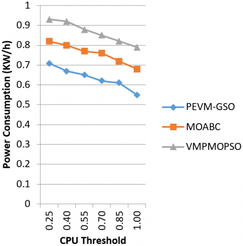
Figure 1. Power consumption for CPU threshold
Figure 1 shows the Power consumption for PEVM-GSO and MOABC techniques when the CPU Threshold is varied [8, 9]. As seen from the figure, the power consumption of PEVM-GSO ranges from 0.71 to 0.55 and the energy consumption of MOABC ranges from 0.82 to 0.68. and the power consumption of VMPMOPSO ranges from 0.93 to 0.79. Hence PEVM-GSO is 16% better than MOABC technique and 27% better than VMPMOPSO technique. Table 3 shows migration values of corresponding threshold values.
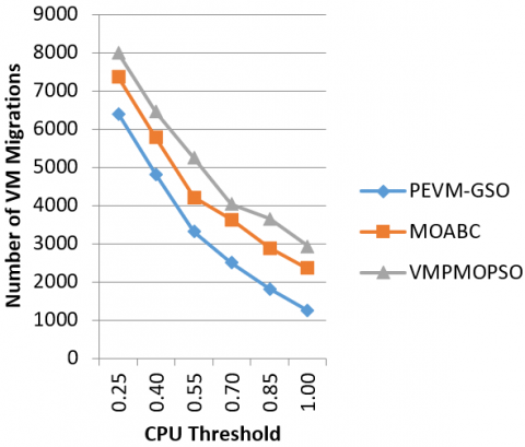
Figure 2 shows the VM Migrations for PEVM-GSO and MOABC techniques when the CPU Threshold is varied. As seen from the figure, the VM Migrations of PEVM-GSO ranges from 6400 to 1250 and the VM Migrations of MOABC ranges from 7345 to 2350 and the VM migration of VMPMOPSO ranges from 7985 to 2945. Hence PEVM-GSO is 28% better than MOABC technique and 38% better than VMPMOPSO technique. Table 4 shows CPU utilization at corresponding threshold values.
Table 3. No of VM migration values for CPU threshold
|
CPU Threshold |
PEVM-GSO |
MOABC |
VMPMOPSO |
|
0.25 |
6400 |
7345 |
7985 |
|
0.40 |
4810 |
5781 |
6454 |
|
0.55 |
3310 |
4210 |
5241 |
|
0.70 |
2480 |
3630 |
4021 |
|
0.85 |
1810 |
2875 |
3652 |
|
1.00 |
1250 |
2350 |
2945 |
Figure 2. Number of VM migrations for CPU threshold
Table 4. CPU utilization values for CPU threshold
|
CPU Threshold |
PEVM-GSO |
MOABC |
VMPMOPSO |
|
0.25 |
70.55 |
65.28 |
55.65 |
|
0.40 |
71.33 |
67.73 |
61.48 |
|
0.55 |
72.52 |
70.36 |
64.98 |
|
0.70 |
73.11 |
71.66 |
68.65 |
|
0.85 |
76.5 |
73.11 |
71.84 |
|
1.00 |
78 |
75.25 |
73.76 |
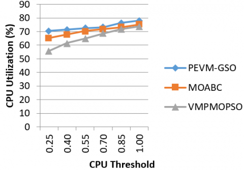
Figure 3. CPU utilization for CPU threshold
Figure 3 shows the CPU Utilization for PEVM-GSO and MOABC techniques [17] when the CPU Threshold is varied. As seen from the figure, the CPU Utilization of PEVM-GSO ranges from 70.55 to 78 and the CPU Utilization of MOABC ranges from 65.28 to 75.25 and CPU utilization of VMPMOPSO ranges from 55.65 to 73.76. Hence PEVM-GSO is 4% better than MOABC technique and 10% better than VMPMOPSO technique [18, 19]. Table 5 shows values of delay for corresponding threshold.
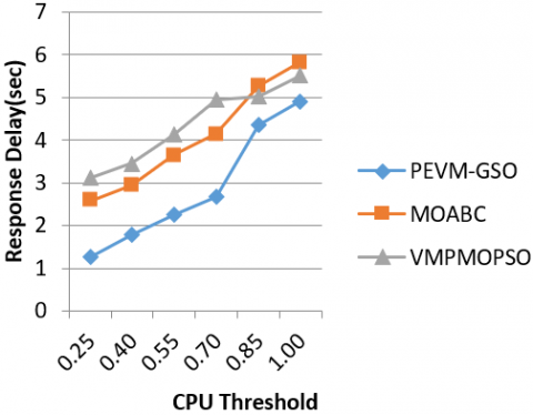
Figure 4 shows the Response Delay for PEVM-GSO and MOABC techniques when the CPU Threshold is varied. As seen from the figure, the Response Delay of PEVM-GSO ranges from 1.25 to 4.92 and the Response Delay of MOABC ranges from 2.58 to 5.82 and the Response delay of VMPMOPSO ranges from 3.12 to 5.52. Hence PEVM-GSO is 33% better than MOABC technique and 37% better than VMPMOPSO technique.
Table 5. Response delay values for CPU threshold
|
CPU Threshold |
PEVM-GSO |
MOABC |
VMPMOPSO |
|
0.25 |
1.25 |
2.58 |
3.12 |
|
0.40 |
1.78 |
2.94 |
3.45 |
|
0.55 |
2.25 |
3.65 |
4.12 |
|
0.70 |
2.66 |
4.15 |
4.95 |
|
0.85 |
4.34 |
5.25 |
5.01 |
|
1.00 |
4.92 |
5.82 |
5.52 |
Figure 4. Response Delay for CPU Threshold
In this paper, power efficient Virtual Machine (VM) migration using GSO algorithm for cloud computing is proposed. In VM selection phase, VMs to be migrated are selected based on their resource utilization and fault probability. In phase-2, optimum number of VMs to be migrated are determined based on the total power consumption. In VM placement phase, GSO is used for finding the target VMs to place the migrated VMs. The fitness function is derived in terms of distance between the main server and the other server, VM capacity and memory size. Then the VMs with best fitness functions are selected as target VMs for placing the migrated VMs. The proposed PEVM-GSO algorithm is implemented in Cloudsim and compared with MOABC algorithm. Performance results show that PEVM-GSO algorithm attains reduced power consumption and response delay with improved CPU utilization, when compared to MOABC algorithm.
[1] Akhter, N., Othman, M., Naha, R.K. (2018). Evaluation of Energy-efficient VM Consolidation for Cloud Based Data Center-Revisited. arXiv preprint arXiv:1812.06255.
[2] AlShayeji, M.H., Samrajesh, M.D. (2017). Energy efficient virtual machine migration algorithm. Journal of Engineering Research, 19-42.
[3] Jena, R.K. (2017). Energy efficient task scheduling in cloud environment. Energy Procedia, 141: 222-227. https://doi.org/10.1016/j.egypro.2017.11.096
[4] Balaji, K., Kiran, P.S., Kumar, M.S. (2020). Resource aware virtual machine placement in IaaS cloud using bio-inspired firefly algorithm. Journal of Green Engineering, 10: 9315-9327.
[5] Li, Z., Yu, X., Yu, L., Guo, S., Chang, V. (2020). Energy-efficient and quality-aware VM consolidation method. Future Generation Computer Systems, 102: 789-809. https://doi.org/10.1016/j.future.2019.08.004
[6] Khajeh-Hosseini, A. (2010). Cloud migration: a case study of migrating an enterprise IT system to IaaS. 2010 IEEE 3rd International Conference on Cloud Computing, pp. 1-5. https://doi.org/10.1109/CLOUD.2010.37
[7] Sayadnavard, M.H., Haghighat, A.T., Rahmani, A.M. (2021). A multi-objective approach for energy-efficient and reliable dynamic VM consolidation in cloud data centers. Engineering Science and Technology, an International Journal. https://doi.org/10.1016/j.jestch.2021.04.014
[8] Elsedimy, E.I., Algarni, F. (2021). Toward enhancing the energy efficiency and minimizing the SLA violations in cloud data centers. Applied Computational Intelligence and Soft Computing, pp. 1-14. https://doi.org/10.1155/2021/8892734
[9] Dad, D., Yagoubi, D.E., Belalem, G. (2014). Energy efficient VM live migration and allocation at cloud data centers. International Journal of Cloud Applications and Computing (IJCAC), 4(4): 55-63. https://doi.org/10.4018/ijcac.201410010516
[10] Thiam, C., Thiam, F. (2019). An energy-efficient VM migrations optimization in cloud data centers. In 2019 IEEE AFRICON, pp. 1-5. https://doi.org/10.1109/AFRICON46755.2019.9133776
[11] Jayamala, R., Valarmathi, A. (2021). An enhanced decentralized virtual machine migration approach for energy-aware cloud data centers. Intelligent Automation And Soft Computing, 27(2): 347-358. https://doi.org/10.32604/iasc.2021.012401
[12] Gu, C., Li, Z., Huang, H., Jia, X. (2018). Energy efficient scheduling of servers with multi-sleep modes for cloud data center. IEEE Transactions on Cloud Computing, 8(3): 833-846. https://doi.org/10.1109/TCC.2018.2834376
[13] Sheetal, A.P., Ravindranath, K. (2021). Cost effective hybrid fault tolerant scheduling model for cloud computing environment. International Journal of Advanced Computer Science and Applications, pp. 416-422. https://doi.org/10.14569/IJACSA.2021.0120646
[14] Krishnanand, K.N., Ghose, D. (2005). Detection of multiple source locations using a glowworm metaphor with applications to collective robotics. In Proceedings 2005 IEEE Swarm Intelligence Symposium, pp. 84-91. https://doi.org/10.1109/SIS.2005.1501606
[15] Li, Z., Huang, X. (2016). Glowworm swarm optimization and its application to blind signal separation. Mathematical Problems in Engineering. https://doi.org/10.1155/2016/5481602
[16] Fahmideh, M., Daneshgar, F.S., Rabhi, F. (2018). A generic cloud migration process model. European Journal of International Systems. https://doi.org/10.1080/0960085X.2018.1524417
[17] Li, Z., Yu, J., Hu, H., Chen, J., Hu, H., Ge, J., Chang, V. (2018). Fault-tolerant scheduling for scientific workflow with task replication method in cloud. In IoTBDS, pp. 95-104.
[18] He, L., Huang, S. (2016). Improved glowworm swarm optimization algorithm for multilevel color image thresholding problem. Mathematical Problems in Engineering. https://doi.org/10.1155/2016/3196958
[19] Alshathri, S., Ghita, B., Clarke, N. (2018). Sharing with live migration energy optimization scheduler for cloud computing data centers. Future Internet, 10(9): 86. https://doi.org/10.3390/fi10090086