RatnaKumari Challa | Kanusu Srinivasa Rao*
© 2021 IIETA. This article is published by IIETA and is licensed under the CC BY 4.0 license (http://creativecommons.org/licenses/by/4.0/).
OPEN ACCESS
Owing to the near connection between object recognition and video processing and picture perception, a lot of research interest has been received in recent years. Standard methods of object detection are focused on manufactured technologies and slow-moving architectures. Fisher Vectors (FV) and Convolutional Neural Networks (CNN) are two picture arrangement pipelines with various qualities. While CNNs have indicated predominant exactness on various order assignments, FV classifiers are normally less exorbitant to prepare and assess. In this paper we propose a mechanism for detection of objects in image based on Fisher kernel and CNN with a PSO optimization technique. Here fisher kernel draws the global or statically features from the image object and CNN is used for local and more complex feature extraction from an image and here we use CNN with PSO to reduce the training complexity. Performance results shows that the proposed model is detect the object better than the existing models.
cnvolutional neural networks (CNN), fisher vectors (FV), PSO, object detection, deep learning, image processing
To gain a total picture understanding, we ought to focus on ordering various pictures, yet additionally attempt to correctly evaluate the ideas and areas of objects contained in each picture. This errand is alluded as object discovery [1], which as a rule comprises of various subtasks, for example, face recognition [2], person on foot location [3] and skeleton identification [4]. As one of the basic PC vision issues, object location can give significant data to semantic comprehension of pictures and recordings, and is identified with numerous applications, including picture arrangement [5, 6], human conduct investigation [7], face acknowledgment [8] and self-ruling driving [9, 10]. In the interim, inheriting from neural systems and related learning frameworks, the advancement in these fields will create neural system calculations, and will likewise impact sly affect object location procedures which can be considered as learning frameworks [11-14]. Be that as it may, because of huge varieties in perspectives, stances, impediments, and lighting conditions, it's hard to impeccably achieve object recognition with an extra object limitation task. So much consideration has been pulled into this field lately [15-18]. The issue meaning of object discovery is to figure out where objects are situated in each picture (object limitation) and which class each object has a place with (object characterization). So, the pipeline of conventional object location models can be for the most part partitioned into three phases: instructive locale determination, highlight extraction and order. Enlightening area determination. As various objects may show up in any places of the picture and have distinctive perspective proportions or sizes, it is a characteristic decision to filter the entire picture with a multi-scale sliding window. Although this thorough technique can discover every single imaginable position of the objects, its deficiencies are likewise self-evident. Because of countless competitor windows, it is computationally costly and delivers such a large number of excess windows. Be that as it may, if just a fixed number of sliding window formats are connected, inadmissible locales might be delivered. Highlight extraction. To perceive various objects, we must remove visual highlights which can give a semantic and vigorous portrayal. Filter [19], HOG [20] and Haar-like [21] highlights are the agent ones. This is because of the way that these highlights can deliver portrayals related with complex cells in human cerebrum [19]. Be that as it may, because of the assorted variety of appearances, light conditions, and foundations, it's hard to physically structure a powerful element descriptor to impeccably depict a wide range of objects. Arrangement. Plus, a classifier is expected to recognize an objective object from the various classifications and to make the portrayals increasingly progressive, semantic, and enlightening for visual acknowledgment. As a rule, the Supported Vector Machine (SVM), AdaBoost and Deformable Part-based Model (DPM) are great decisions. Among these classifiers, the DPM is an adaptable model by joining object parts with disfigurement cost to deal with extreme misshapenness. In DPM, with the guide of a graphical model, deliberately planned low-level highlights and kinematic ally propelled part disintegrations are consolidated. What's more, discriminative realizing of graphical models considers constructing high-accuracy part-based models for an assortment of object classes. In light of these discriminant neighborhood highlight descriptors and shallow learnable models, cutting edge results have been gotten on PASCAL VOC object recognition rivalry and continuous inserted frameworks have been acquired with a low weight on equipment. Be that as it may, little gains are gotten during 2010-2012 by just structure troupe frameworks and utilizing minor variations of effective strategies [15]. This reality is because of the accompanying reasons: 1) the age of competitor bouncing boxes with a sliding window procedure is repetitive, wasteful and erroneous. 2) The semantic hole can't be connected by the mix of physically designed low-level descriptors and discriminatively prepared shallow models.
1.1 PSO
For example, flocks of birds or schools of fish are examples of intelligent collective behavior that may be driven by particle swarm optimization (PSO), a population-based stochastic optimization method that uses a population-based stochastic optimization algorithm. Since it was first introduced in 1995, it has undergone a plethora of improvements.
The construction of complex networks and the functioning of these networks contribute to a rise in computational complexity. Among the limitations of the particle swarm optimization (PSO) method include its tendency to slip into a local optimal state in high-dimensional space, as well as its relatively slow convergence rate throughout the repetitive process.
1.2 Fisher kernel
The Fisher kernel, named after Ronald Fisher, is a function in statistical classification that determines the similarity of two items based on sets of measurements for each object and a statistical model. The class for a new item (whose true class is unknown) may be approximated by minimizing, across classes, an average of the Fisher kernel distance between the new object and each existing member of the given class, according to a classification method.
1.3 Convolution Neural Network
CNNs (Convolutional Neural Networks) are used in a wide variety of applications. It's the most widely used deep learning architecture, without a doubt. Deep learning has recently seen a resurgence in popularity, thanks to convnets' enormous popularity and efficacy. Of 2012, AlexNet sparked a surge in interest in CNN, and that enthusiasm has only increased since then. Researchers advanced from the 8-layer AlexNet to the 152-layer ResNet in only three years. For every image-related issue, people increasingly turn to CNN. They outperform the competitors when it comes to precision. There are many more uses as well, such as using recommender systems or natural language processing. Comparing CNN to its predecessors, the most significant benefit is that it automatically identifies the most essential characteristics without human oversight. Using numerous images of cats and dogs, for example, it can figure out what makes each one unique. The computational efficiency of CNN is very impressive. It performs parameter sharing and specific convolution and pooling techniques. As a result, CNN models may be used on any device, making them more appealing to a wider audience.
In this paper we propose a mechanism for detection of objects in image based on Fisher kernel and CNN with a PSO optimization technique. Here fisher kernel draws the global or statically features from the image object and CNN is used for local and more complex feature extraction from an image and here we use CNN with PSO to reduce the training complexity. The rest of the paper is organized as follows section-2 details the state of the art, section-3 illustrates the proposed work, section-4 gives the results and discussion, and section-5 concludes the paper.
In the nineteenth century large numbers of advanced imaging or computerised image management systems were developed. A few inquiries were transmitted on satellite images, improvements in the instructions on wire-photography, clinical imagery, camera telephones, identification of characteristics and software upgrades [1].
Chen et al. [14] FanS-CNN: Target exploration subcategory memorial systems Deep coevolutionary neural system (CNN) and surround proposal have made advances to the entity position after the latter. Although the highlights of the discriminative artefacts are observed by means of a profound CNN, the vast intra-class variety of the item recognition also involves the show. In order for developers to consider the intra-class differ problem of the item, they suggest a sub-category mindful CNN (S-CNN). In this new illustration discussing the most severe edge grouping technique, the preparedness assessments will first be categorised in different sub-categories. A multi-part locator for Aggregated Channel Functionality (ACF) is then ready for increasingly inactive planning testing, where each section of ACF contrasts itself with a bunch of subcategories.
Nakadate et al. [15] examined the utilization of computerized picture preparing strategies for electronic spot design interferometry. An advanced TV-picture preparing framework with a huge edge memory enables them to perform exact and adaptable tasks, for example, subtraction, summation, and level cutting. Computerized picture preparing procedures made it simple contrasted with simple systems with create high differentiation borders.
Robinson [16] talked about the attributes of the iterative picture reclamation strategy altered by the deblurring technique through an investigation in recurrence space. An iterative technique for settling concurrent direct conditions for picture rebuilding has an intrinsic issue of union. The presentation of the system called "deblur" tackled this combination issue. This deblurring technique likewise served to stifle commotion enhancement. Two-dimensional re-enactments utilizing this strategy showed that a boisterous picture corrupted by straight movement can be all around re-established without recognizable commotion enhancement.
Bishop et al. [5] regions of use were inspected where the utilization of a framework dependent on an irregular access edge store has empowered a handling calculation to be created to suit a particular issue. Besides, it empowered programmed examination to be performed with perplexing and loud information. The applications considered were strain estimation by dot interferometry, position area in three tomahawks, and shortcoming discovery in holographic non-destructive testing. A concise depiction of every issue is exhibited, trailed by a portrayal of the preparing calculation, results, and timings.
Chatfield et al. [7] exhibited an overview of thresholding strategies and refreshed the prior study work. An endeavour was made to assess the exhibition of some programmed worldwide thresholding techniques utilizing the standard capacities, for example, consistency and shape measures. The assessment depended on some true pictures.
Lee et al. [17] explored distinctive impediment situation and performed following under six diverse video reproduction techniques. They assessed the presentation utilizing SFDA (Sequence Frame Detection Accuracy). Besides, they exhibited mean move, molecule and Kalman sifting for assessing following execution. Furthermore, they found that for self-assertive development of the article Particle Filter (PF) neglects to perform successfully.
Kim [18] objects are arbitrarily picked by a client are followed utilizing SIFT highlights what's more, a Kalman channel. In particular, they focused on following human, vehicle, or pre-learned objects. The items are amassed, abused the figuring out how to effectively track items notwithstanding when the articles missing for certain edges. Be that as it may, this investigation requirements to concentrate on higher goals with finding the area of stationary articles.
Nagendran et al. [19] proposed a strategy for adequately following moving articles in recordings. They utilized relative change for settling the video. At that point separate these highlights utilizing outline determination. Further, they utilized Kalman channel and Gaussian blend model for following the moving articles. Nonetheless, this investigation needs to focus on decrease of computational time just as expanding acknowledgment for different classes.
Poschmann et al. [20] built up a PF approach utilizing combination strategy for expanding versatile following strength. This exploration relatively broke down the different variations and showed the practicality of applying a system for a real-world situation. The real trouble recognized in this exploration is the edge for learning is critical which will be either excessively high or excessively low. Another issue distinguished is in view of video, edge isn't refreshed whether terrible or none. The expressed issue can be overwhelmed by misuse of versatile edge practicality in proposed approach or else need to locate a substitute path to this test.
Mei and Lin [21] proposed a LAD (least total deviation) learning technique dependent on a performing various tasks and Multiview method for following. The proposed methodology utilizes PF for viable item following. The proposed methodology is actualized under four various highlights of items like shading histogram, force, LBP (Local twofold examples) and HOG (Histogram of Oriented Gradients). Further, this examination is analyzed under a few testing circumstances like clamor accessibility in genuine world, manufactured boisterous grouping, accessibility of arrangement out in the open and complete following of accessible informational collections. The re-enacted outcomes show that proposed strategy was given the upside of Multiview information taking care of and task exception. Further, the proposed approach displays prevalent execution for similar assessment of existing following techniques.
The BPnP [22] is a network module that approximates backpropagation gradients by guiding variations using a PnP solver. If the optimization block is discrete, the PnP solver's gradients may be computed implicitly. Despite incorporating a PnP solver layer, the proposed method may effectively train embeddings for problems such as architecture from motion, geometric collimation, and posture prediction [23]. A BPnP-based trainable pipeline with feature map loss and 2D–3D reprojection defects increases pose estimation accuracy.
In this paper we propose a mechanism for detection of objects in image based on Fisher kernel and CNN with a PSO optimization technique. Here fisher vector draws the global or statically features from the image object and CNN is used for local and more complex feature extraction from an image and here we use CNN with PSO to reduce the training complexity.
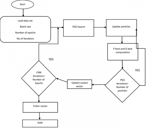
Figure 1 shows the proposed model Architecture of object detection using FA-PSOCNN.
Figure 1. Architecture of object detection using FA-PSOCNN
3.1 PSO
By using particles as a competition arrangement for these particles to travel through spaces, as seen in numerical conditions, this changing of locations is caused by their own best place and directed to the best place worldwide in certain search spaces discovered and concurred by various particles. It maximises the mechanism by using particles as a competitors' arrangement. The probability of this estimate would be to recreate the social behaviour, using any of the health abilities, of flying rushes and fish colleges, which seem like a suitable place for footsteps.
The swarm particles work together to achieve the optimal value, as demonstrated by the data they exchange. Each molecule in the swarm has a near best (Pbest) location, the least costly that has been obtained in the past. In addition to this, it is good to control all the particles against the world-wide ideal through the swarm, which is considered worldwide best location. Condition (1) is to determine the molecule's pace and condition (2) is used to measure the molecule state.
vn+1=vn+c1r1(Pbest-xn)+c2r2(Gbest-xn)
xn+1=xn+vn+1
where, c1 and c2 are two constants and r1 and r2 are irregular qualities. The molecule is refreshed at every cycle utilizing its neighborhood best accomplished position "Pbest" and the worldwide best position in the swarm "Gbest".
3.2 Features
We propose in this paper a combined strategy that takes use of two recent significant state of the art systems. It was proposed to use the Fisher Kernel in conjunction with a Gaussian mixture model as the underlying generative model. A strong multilayer discriminative model is trained in order to provide findings that are at the cutting edge of the field. In order to build a classification system that selects the best of the two methods, it is tempting to combine them in order to produce a classifier that is superior than the two approaches combined. Using random CNNs, it is shown how to extract FK based features and how to utilize these features as image descriptors in this paper.
3.3 Expressing generative likelihood from a CNN
In order to be able to construct a Fisher Kernel from a probability model, it is first required to define the loglikelihood function of the probability model. Considering that the CNN is a discriminative model, there should not be a method to define the function P (T|$\emptyset$) (recall that T are observable data variables, such as pictures, and that is the collection of CNN's parameters) mathematically. The SoftMax layer at the top of the CNN is examined in order to demonstrate that there is a way of expressing the generative loglikelihood function. Remember that the CNN SoftMax function has the following appearance:
$p\left(C_{k} / x, \emptyset\right)=\left(\exp \left(\left(w_{k}\right)^{T} x^{1}+b_{k}\right)\right) /\left(\sum_{j} \exp \left(\left[w_{k}\right]^{T} x^{1}+b_{j}\right)\right)$ (1)
where, Ck denotes the k-th class, wk and bk denote the tunable weights and bias, respectively, of the class. If we consider CNN, T is an image and T are activations of the penultimate CNN layer, where T is the picture.
As previously shown in Ponce et al. [5], the SoftMax function may be seen as an expression for the Bayes rule with tunable parameters wk, as illustrated in Bose et al. [6]. In addition, bk:
$p\left(C_{k} / x, \emptyset\right)=\frac{\exp \left(w_{k}{ }^{T} x^{1}+b_{k}\right)}{\sum_{j} \exp \left(w_{k}{ }^{T} x^{1}+b_{j}\right)}=\frac{p\left({x} / \emptyset, C_{k}\right) p\left(\emptyset, C_{k}\right)}{\sum_{j} p\left({x} / \emptyset, C_{j}\right) p\left(\emptyset, C_{j}\right)}=p\left({ }{C_{k}} / \emptyset, x\right)$ (2)
This also demonstrates that the joint probability P (T, $\emptyset$, Ck) (which is equal to the nominator of Eq. (2) is equal to:
$p\left(C_{k}, \emptyset, x\right)=\exp \left(w_{k}^{T} x^{1}+b_{k}\right)=p\left({x} / \emptyset, C_{k}\right) p\left(\emptyset, C_{k}\right)$ (3)
One need for constructing a generative loglikelihood function is that one be able to define the generative probability P (T|Ω), where Ω is an acronym for the set of model parameters that has just been introduced. With respect to CNN, it is suggested to include the variables C1...CK into the set of model parameters (i.e, =Ω, C1...CK) in order to represent the likelihood of a set of pictures Ω conditional on the parameter (i.e., C1...CK). P (T|Ω) is defined as follows at this point:
$P\left(x / \Phi, C_{1}, \ldots, C_{k}\right)=P(x / \Omega)=\frac{P\left(x, C_{1}, \ldots, C_{k}, \Phi\right)}{P\left(C_{1}, \ldots, C_{k}, \Phi\right)}=\frac{P(\Phi, x) \prod_{k=1}^{K} P\left(C_{k} / \Phi, x\right)}{P\left(C_{1}, \ldots, C_{k}, \Phi\right)}$ (4)
here, it is assumed that the probabilities P (P (C1|$\emptyset$, T)... P (CK |$\emptyset$, T)) are independent of one another. Keep in mind that this assumption comes from the probabilistic interpretation of the SoftMax activation function, which is provided in Eq. (2) and has the following formula:
Assuming that samples P (T|$\emptyset$, C1... CK) are independent P (T|$\emptyset$, C1, ..., CK ) then becomes:
$P\left(X / \Phi, C_{1}, \ldots, C_{k}\right)=\prod_{i=1}^{n} P\left(x_{i} / \Phi, C_{1}, \ldots, C_{k}\right)$ (5)
It would be necessary to proceed in accordance with the Fisher Kernel framework at this stage in order to get the formula for the derivative of the loglikelihood of P (T|$\emptyset$, C1, ..., CK). However, there are a number of considerations that make this step very difficult:
P (C1,..., CK, T) and P (C1,..., CK, $\emptyset$) are both unknown. Neither the probabilities P (T, $\emptyset$) nor the probability P (C1, C2,..., CK, $\emptyset$) from Eq. (4) are known. Although it is feasible to assume a uniform prior over P (C1,..., CK,) in the Fisher Kernel setting, the prior P (T) is dependent on the data T, which is a feature that cannot be ignored in the Fisher Kernel setup.
Derived from the loglikelihood Although there may be a way to get around the problem of unknown probabilities, getting the derivatives of the loglikelihood function with respect to the parameter set would be a very difficult job to do.
As an alternative to creating unreasonable assumptions that would aid us in getting the final evaluable formulation of P (T|$\emptyset$, C1,...), we define our own function f($\emptyset$, T, C1,...) that has characteristics comparable to the probability P (T|$\emptyset$, C1,..., CK), which has the following features:
$\wedge\left(x, \Phi, C_{1}, \ldots, C_{k}\right)=\prod_{k=1}^{K} P\left(x, \Phi, C_{k}\right)$ (6)
Function Λ in our formulation of Fisher Kernel-based features replaces the term probabilities with the term function. P (T|$\emptyset$, C1, ..., CK).
The FK classifier makes use of derivatives of the generative loglikelihood function in order to classify data based on its parameters. Because we are using a function that we have defined, Λ(T, $\emptyset$, C1, ..., CK), As pseudo-likelihood is defined as L(T|$\emptyset$, C1, ..., CK), we refer to the et pression that is the equivalent to the generative likelihood.
$\hat{\mathcal{L}}_{\wedge}\left(X, \Phi, C_{1}, \ldots, C_{k}\right)=\prod_{i=1}^{n} \wedge\left(x_{i}, \Phi, C_{1}, \ldots, C_{k}\right)$ (7)
Please keep in mind that in the case of CNNs, the set of samples T really contains just one observation, which is the image Ti, which means that in our instance the number of observations is equal to one. Input the contents of Eq. (3) into the pseudo-likelihood formula Eq. (7) and you will get the following result:
$\hat{\mathcal{L}}_{\wedge}\left(X, \Phi, C_{1}, \ldots, C_{k}\right)=\prod_{i=1}^{n} \prod_{k=1}^{K} \exp \left(\omega_{k}^{T} \hat{x}+b_{k}\right)$ (8)
The pseudo-loglikelihood function corresponding to Eq. (8) is constructed by taking the logarithm of the equation.
$\log \hat{\mathcal{L}}_{\Lambda}\left(X, \Phi, C_{1}, \ldots, C_{k}\right)=\sum_{i=1}^{n} \sum_{k=1}^{K} \omega_{k}^{T} \hat{x}_{i}+b_{k}$ (9)
In order to get Fisher Kernel-based features, it is necessary to take a derivative of the function log (T,$\emptyset$, C1... CK) with regard to its Parameters $\emptyset$, C1... CK).
Please keep in mind that the derivatives of Eq. (9) are not the correct Fisher Kernel features since we choose to substitute probabilities P (T|$\emptyset$, C1,...,Ck) with probability measures Λ(T, $\emptyset$, C1, ..., CK) that cannot be considered as generative probability measures. However, our choice of Λ(T, $\emptyset$, C1, ..., CK) may be acceptable in certain circumstances.
This method's goal is to assign larger values of P (T∅ |, C1,...CK) to pictures T that are more likely than other images to be seen. The product of normalised class posteriors P (T, $\emptyset$, ck) is computed by our function P (T, $\emptyset$, ck). As a result, when P (T, y, and c) are all raised, the value of achieves a maximum. From the point of view of, the pictures that are most likely to emerge are those that include items from the classes C1 through C6. As a rationale for our selection of the function as an acceptable substitute for P (T| $\emptyset$, C1,..., CK), we hope that the fact that it assigns high values to pictures that include real visual objects may be considered.
From the perspective of the Fisher Kernel, the gradients of the loglikelihood should take on a “meaningful” shape when plotted. This implies that their directions should be constructed in such a way that linear classification may be performed in this space. It is necessary to utilise the gradients of models that have been trained to optimise generative loglikelihoods in the case of the Fisher Kernel. The fact that the loglikelihood of the model reaches its maximum ensures that this feature of the gradient directions is preserved. However, it is not immediately clear if the gradients of the aforementioned pseudo-loglikelihood show the same property as the gradients of the aforementioned pseudo-loglikelihood. In spite of the fact that we do not provide any theoretical reasons, the empirical findings presented in Section 5 demonstrate that our Fisher Kernel-based features are appropriate for linear classification.
Another advantage of is the simplicity of the pseudo-loglikelihood formula Eq. (9) that is produced as a consequence of it. Because the exponential components have been removed from the equation, the statement is reduced to the form of a simple sum of linear functions. The process of obtaining its derivative is therefore straightforward.
As a theoretical issue, the fact that n=1 in formula Eq. (7) may be viewed as problematic, since the Fisher Kernel was initially designed to compare sets of samples T that often include more than one element. To address this problem, for example, random cropping or flipping of the original picture T may be performed and then added to the set T. This would be an additional stage in the process of developing our suggested technique, and it is not addressed in detail in this thesis. Remember that the variables T and T are ambiguous in this specific instance since they both represent the same picture, which is T.
For the reasons stated above, the gradients of cannot be considered as Fisher Kernel features, and this conclusion is supported by the data. We suggest that the sole difference between the Fisher Kernel and our proposed approach is that we substitute our own function for the probability P (c1,...,ck) in the Fisher Kernel. As a result, due of the striking similarity between the gradients of Fisher Kernel based features and the original approach, we have chosen to refer to them as such throughout this thesis.
3.4 Obtaining Fisher Kernel-based characteristics from CNN
Using the gradients of the pseudo-loglikelihood generated by a CNN in conjunction with an SVM solver and applying it to image classification is shown in the next section. Equation Eq. (9) contains the pseudo-loglikelihood formula, which may be found here. Similarly to the Fisher Kernel, the kernel function Kj compares two sample sets Ti and Tj using gradients of the pseudo-loglikelihood and using gradients of the pseudo-loglikelihood.
$K_{\Lambda}\left(X_{i}, X_{j}\right)=U_{X_{i}}^{T} I^{-1} U_{X_{j}}$ (10)
When applied to the CNN Eq. (9) with respect to its parameters Ti, UT is denoted by the derivative of the pseudo-log likelihood of the CNN Eq. (9) with respect to its parameters Ti.
$U_{x}=\nabla \sigma \log L / x_{i}$ (11)
Also feasible is to use the Cholesky decomposition of the matrix I once again and represent the kernel function K(Ti, Tj ) as the product of two column vectors YTi and Tj, as shown in the following example. where
$K_{A}\left(x_{t}, x_{j}\right)=y^{t} x_{i} y x_{j}$ (12)
$Y_{x}=L U_{x} I=L^{1} L$ (13)
Following the acquisition of YT, the following l2 normalisation is performed:
$Y^{l 2}{ }_{x}=\frac{Y_{x}}{\left[Y_{x}^{2}\right]}$ (14)
It should be noted that, for the sake of simplicity, the vector Yl2 shall be represented by the symbol T. The CNN-FK classifier, which is created by utilising derivatives of the pseudo-loglikelihood of CNN, will be referred to as the CNN-FK classifier, and the vectors T Fisher Kernel based features, or simply CNN-FK features, will be referred to as CNN-FK features.
4.1 COCO data set
Microsoft COCO Folder: Folder comprising 80 categories of items Microsoft COCO entity recognition. We obey to use 80k training pictures and 60k to evaluate [10].
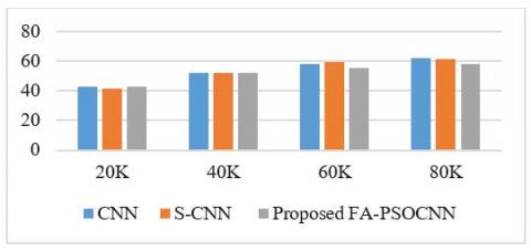
Figure 2 shows the training time comparison of CNN and state of the art S-CNN and proposed FA-PSOCNN with respect to number of data samples. Here CNN takes more time initially and also time increasing with respect to data set size. And state of the art S-CNN takes better time with respect to data set. But proposed mechanism takes less time with respect to other two mechanisms while increasing the data set size also.
Figure 2. Training time (Ms)
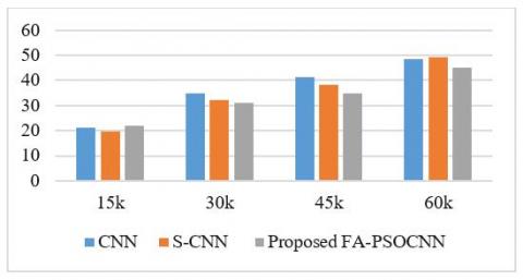
Figure 3. Testing time (Ms)
Figure 3 shows the testing time comparison of CNN and state of the art S-CNN and proposed FA-PSOCNN with respect to number of data samples. Here CNN takes more time initially and also time increasing with respect to data set size. And state of the art S-CNN takes better time with respect to data set. But proposed mechanism takes less time with respect to other two mechanisms while increasing the data set size also.
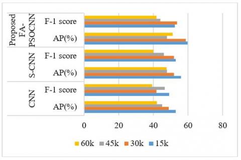
Figure 4 displays the AP and F1-score comparison values. In calculating the accuracy of object detector such as CNN, S-CNN and the proposed CNN, AP (average precision) is a common metric. The average accuracy measures the average recall value of 0 to 1. F1 score blends accuracy and reminder in conjunction with a similar optimistic rating-The F 1 value can be called a weighted average accuracy and reminder. The process suggested here is beyond the normal CNN and state-of-the-art S-CNN level.
Figure 4. AP% and F1-score
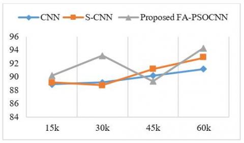
Figure 5. Accuracy%
Figure 5 shows the accuracy of proposed CNN and standard CNN and S-CNN. Accuracy refers to the exact detection of objects from an image. Here proposed mechanism outperformed the state-of the artwork. Detection accuracies increase with respect to the number of images increases.
An improved hybrid technique for obtaining Fisher Kernel based statistics from convolutional neural networks was given, which was combined with a PSO optimization mechanism that was used to the CNN's training process in this study. It has been rigorously tested on the COCO picture classification task as well as the object recognition challenge, with good results in both instances. When constructed on top of Fisher Kernel based feature vectors, an image classification process may provide results that are similar to those produced by current state of the art techniques in the field. This method has also been proven to enhance the performance of the conventional CNN image classification architecture, which has been shown before.
[1] Alexe, B., Deselaers, T., Ferrari, V. (2012). Measuring the objectness of image windows. IEEE Transactions on Pattern Analysis and Machine Intelligence, 34(11): 2189-2202. https://doi.org/10.1109/CVPR.2010.5540226
[2] Babenko, A., Slesarev, A., Chigorin, A., Lempitsky, V. (2014). Neural codes for image retrieval. In European Conference on Computer Vision, pp. 584-599. https://doi.org/10.1007/978-3-319-10590-1_38
[3] Bengio, Y. (2009). Learning deep architectures for AI. Now Publishers Inc. https://doi.org/10.1561/2200000006
[4] Bengio, Y., Simard, P., Frasconi, P. (1994). Learning long-term dependencies with gradient descent is difficult. IEEE Transactions on Neural Networks, 5(2): 157-166. https://doi.org/10.1109/72.279181
[5] Ponce, J., Hebert, M., Schmid, C., Zisserman, A. (Eds.). (2007). Toward Category-Level Object Recognition (Vol. 4170). Springer.
[6] Boser, B.E., Guyon, I.M., Vapnik, V.N. (1992). A training algorithm for optimal margin classifiers. In Proceedings of the Fifth Annual Workshop on Computational Learning Theory, pp. 144-152. https://doi.org/10.1145/130385.130401
[7] Chatfield, K., Simonyan, K., Vedaldi, A., Zisserman, A. (2014). Return of the devil in the details: Delving deep into convolutional nets. arXiv preprint arXiv:1405.3531. https://doi.org/10.5244/C.28.6
[8] Cheng, M.M., Zhang, Z., Lin, W.Y., Torr, P. (2014). BING: Binarized normed gradients for objectness estimation at 300fps. In Proceedings of the IEEE Conference on Computer Vision and Pattern Recognition, pp. 3286-3293. https://doi.org/10.1109/CVPR.2014.414
[9] Gokberk Cinbis, R., Verbeek, J., Schmid, C. (2013). Segmentation driven object detection with fisher vectors. In Proceedings of the IEEE International Conference on Computer Vision, pp. 2968-2975. https://doi.org/10.1109/ICCV.2013.369
[10] Csurka, G., Dance, C., Fan, L., Willamowski, J., Bray, C. (2004). Visual categorization with bags of keypoints. In Workshop on Statistical Learning in Computer Vision, ECCV, 1(1-22): 1-2.
[11] Dalal, N., Triggs, B. (2005). Histograms of oriented gradients for human detection. In 2005 IEEE Computer Society Conference on Computer Vision and Pattern Recognition (CVPR'05), pp. 886-893. https://doi.org/10.1109/CVPR.2005.177
[12] Deng, J., Dong, W., Socher, R., Li, L.J., Li, K., Li, F.F. (2009). Imagenet: A large-scale hierarchical image database. In 2009 IEEE Conference on Computer Vision and Pattern Recognition, Miami, FL, USA, pp. 248-255. https://doi.org/10.1109/CVPRW.2009.5206848
[13] Donahue, J., Jia, Y., Vinyals, O., Hoffman, J., Zhang, N., Tzeng, E., Darrell, T. (2014). Decaf: A deep convolutional activation feature for generic visual recognition. In International Conference on Machine Learning, pp. 647-655. http://proceedings.mlr.press/v32/donahue14
[14] Chen, T., Lu, S., Fan, J. (2017). S-CNN: Subcategory-aware convolutional networks for object detection. IEEE Transactions on Pattern Analysis and Machine Intelligence, 40(10): 2522-2528. https://doi.org/10.1109/TPAMI.2017.2756936
[15] Nakadate, S., Tokudome, T., Shibuya, M. (2004). Displacement measurement of a grating using moire modulation of an optical spectrum. Measurement Science and Technology, 15(8): 1462. https://doi.org/10.1088/0957-0233/15/8/005
[16] Robinson, D.W. (1983). Automatic fringe analysis with a computer image-processing system. Applied Optics, 22(14): 2169-2176. https://doi.org/10.1364/AO.22.002169
[17] Lee, B.Y., Liew, L.H., Cheah, W.S., Wang, Y.C. (2012). Measuring the effects of occlusion on kernel based object tracking using simulated videos. Procedia Engineering, 41: 764-770. https://doi.org/10.1016/j.proeng.2012.07.241
[18] Kim, Y.M. (2007). Object tracking in a video sequence. CS, 229: 366-384.
[19] Nagendran, A., Dheivasenathipathy, N., Nair, R.V., Sharma, V. (2014). Recognition and tracking moving objects using moving camera in complex scenes. International Journal of Computer Science, Engineering and Applications, 4(2): 31. https://doi.org/10.5121/ijcsea.2014.4203
[20] Poschmann, P., Huber, P., Rätsch, M., Kittler, J., Böhme, H.J. (2014). Fusion of tracking techniques to enhance adaptive real-time tracking of arbitrary objects. Procedia Computer Science, 39: 162-165. http://dx.doi.org/10.1016/j.procs.2014.11.025
[21] Mei, X., Ling, H. (2011). Robust visual tracking and vehicle classification via sparse representation. IEEE Transactions on Pattern Analysis and Machine Intelligence, 33(11): 2259-2272. http://dx.doi.org/10.1109/TPAMI.2011.66
[22] Chen, B., Parra, A., Cao, J., Li, N., Chin, T.J. (2020). End-to-end learnable geometric vision by backpropagating PnP optimization. In Proceedings of the IEEE/CVF Conference on Computer Vision and Pattern Recognition, pp. 8100-8109. arXiv:1909.06043
[23] Gopil, A., Narayana, V.L. (2017). Protected strength approach for image steganography. Traitement du Signal, 34(3-4): 175-181. http://dx.doi.org/10.3166/ts.34.175-181