Xiaogai Shen
© 2020 IIETA. This article is published by IIETA and is licensed under the CC BY 4.0 license (http://creativecommons.org/licenses/by/4.0/).
OPEN ACCESS
To satisfy the demand of virtual simulation (VS) teaching system for storage capacity and computing power, it is of great significance to probe deep into the VS system oriented to cloud service (CS). This paper designs a CS-based VS teaching system, drawing on the relevant results on distributed VS system, the formalization of VS system architecture, and the semantic organizability of VS system. Firstly, the functional requirements of the CS-based VS teaching system were analyzed, and decomposed into three layers, namely, goal, function type, and function name. Then, a dynamic model of CS-based VS teaching system was constructed, whose simulation accuracy and precision were verified through experiments. The experimental results demonstrate the excellent simulation performance of the proposed system. The research findings provide reference for applying CS system design in other fields.
virtual simulation (VS), cloud service (CS), VS teaching system, simulation system design
Virtual simulation (VS) aims to analyze the system architecture and functions of the object, providing a reference for the decision-making of applications based on that object. The VS process can be broken down into four stages: object modeling, model structuring and programming, model running and verification, and comparative analysis of experimental results [1-5].
The VS has been widely used in the field of teaching. Teachers and researchers rely on the VS to explore actual complex nonlinear systems and use them to teach students. If the target system has complex functions, it will be complicated and compute-intensive to simulate the system [6-8]. The massive data have challenged various aspects of VS teaching system applications, ranging from program development, architecture design, to the accuracy and combination of simulation elements.
As a new computing service model, cloud service (CS) has become a research hotspot [9-12]. CS and VS are two research fields with different purposes and contents [13-15]. But it is CS that provides the basic platform and application environment for the VS based on logical framework. Currently, there is no unified standard for CS platforms of VS teaching. Many key details need to be solved before applying CS to VS teaching [16, 17].
The existing studies on CS-based VS mainly focus on distributed VS system, the formalization of VS system architecture, and the semantic organizability of VS system [18, 19]. Most of the VS systems on the market are developed under the high-level architecture (HLA). After extending the HLA, Schaefer, Schaefer et al. [20] designed simulation systems for application scenarios like high-energy chemical data analysis, tide warning, and ultraviolet lighting analysis. Bajpai et al. [21] introduced the Cosim-Grid, a simulation grid project of China National Grid (CNGrid) for industrial production scenarios (e.g. product supply, product output, and manufacturing cycle), and emphasized that the project can complete such services as resource allocation to varied production and marketing modes, and management of supply chain members. Loukriz et al. [22] designed the Aurora system to overcome the performance defect of distributed simulation system in CS environment; through the system, the workers that undertake lots of computing tasks are controlled through the master, and all cached VS data and processes are integrated into one data packet to be exchanged between different simulation elements.
On the formalization of VS system architecture, Maeda et al. [23] developed a universal hierarchical modular VS framework called discrete event VS (DEVS) for the numerous discrete events in the real world, and successfully described the time-varying effects and associations between the modules within the object. Ghosh et al. [24] put forward a parallel DEVS modeling paradigm oriented to the logic process paradigm, which makes up the insufficiency of DEVS in depicting the execution capability of parallel events.
On the semantic organizability of VS system, Ferraresi et al. [25] proposed a hierarchical extended simulation model based on high-level concepts for combined discrete events, and demonstrated that the proposed model has high accuracy and strong ability to handle complex problems.
To satisfy the demand of VS teaching system for storage capacity and computing power, it is of great significance to probe deep into the VS system oriented to CS, and rationalize the description and data processing of the object. Thus, this paper designs a VS teaching system based on CS. Firstly, the functional requirements of the CS-based VS teaching system were analyzed, and decomposed into three layers, namely, goal, function type, and function name. Then, a dynamic model of the CS-based VS teaching system was established, plus the sequence diagram of the modeling process. After that, the simulation accuracy and precision of the proposed system were verified through experiments. The experimental results show that the proposed system is fast in response, and powerful in resource management and operation execution.
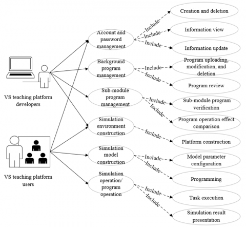
The CS-based VS teaching system mainly targets program developers and users. Figure 1 shows the use cases of VS teaching system functions. Five kinds of functions can be summarized for VS teaching system:
(1) The CS-based VS teaching system needs to support four basic functions: interfacing module interactions; managing developer and user configurations; environment design and program running; data collection and processing.
(2) Four levels of interfaces should be provided for the interactive services between modules: control interface, connection interface, data interface, and basic interface.
(3) The configurations of developers and users should be managed in four aspects: account and password; program uploading and modification; platform parameters and strategies; type and number of tasks.
(4) The cloud simulation service engine and its functions should be expanded and packaged through environment design and program running.
(5) The data on VS teaching system should be collected, processed, and presented accurately.
Figure 1. The use cases of VS teaching system functions
The specific functions of CS-based VS teaching system are as follows:
Layer 1 (goal)
D={D1, D2, D3, D4}={interfacing module interactions, managing developer and user configurations, environment design and program running, data collection and processing}
Layer 2 (type)
D1={D11, D12, D13, D14}={control interface, connection interface, data interface, basic interface};
D2={D21, D22, D23, D24, D25, D26, D27, D28}={user creation and deletion, user information view, user information update, user simulation operation, managing program upload and configuration modification, managing platform parameter configuration, managing computer resource configuration, managing type and number of tasks}
D3={D31, D32}={environment design, program running}
D4={D41, D42, D43}={data collection, data processing, data presentation}
Layer 3 (name)
D11={D111, D112, D113, D114, D115, D116}={platform, task, program configuration interface, user control command management interface, program operation control interface, simulation result output and query interface}
D12={D121, D122, D123}={simulation element combination interface, task scheduling and configuration interface, simulation module control interface}
D13={D131, D132, D133, D134, D135}={main task interface, simulation data library interface, task creation interface, task execution interface, simulation element and module scheduling management interface}
D14={D141, D142}={simulation module output data interface, platform output data interface}
D21={D211, D212}={user creation, user deletion}
D22={D221, D222, D223, D224}={viewing user basic information, viewing user program information, viewing user model information, viewing user program running state}
D23={D231}={updating user basic information}
D24={D241, D242}={running user simulation, stopping user simulation}
D25={D251, D252, D253, D254}={program uploading, program modification, program deletion, program query}
D26={D261, D262}={simulation database parameter configuration, computer parameter configuration}
D27={D271, D272, D273, D274, D275}={processor resource allocation, memory resource allocation, bandwidth resource allocation, storage resource allocation, task scheduling priority}
D28={D281, D282, D282}={type of task type, execution time of task, number of tasks}
D31={D311, D312, D313, D314, D315}={construction of platform, determination of simulation principle, program preparation, comparison of experimental results, program validation}
D32={D321, D322, D323, D324}={starting task, pausing task, resuming task, ending task}
D41={D411, D412, D413}={CS data, energy consumption data, task execution time data}
D42={D421, D422}={data analysis algorithm, data processing algorithm}
D43={D431, D432}={graphic presentation of simulation result, tabular presentation of simulation result}
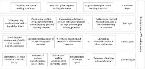
Figure 2. The hierarchical structure of CS-based VS teaching system
According to the requirements of tasks, the CS-based VS teaching system should be able to remove the coupling between sub-modules, simulation tools, sub-nodes of program running, and connection nodes of simulation elements, such as to ensure the efficient and reliable operation of the program. Figure 2 illustrates the hierarchical structure of CS-based VS teaching system. It can be seen that the key techniques in the dynamic modeling of the CS-based system are virtualizing and standardizing the target simulation elements of CS.
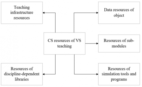
The basic operation process of the dynamic model is as follows: After different users upload the program, the CS center will parse the requirements of the program for computer resources, simulation element combination, and sub-module scheduling, select and call relevant simulation elements and sub-modules from the simulation libraries as per the parse results, and combine these elements and sub-modules to construct the main task. Figure 3 gives the simplified architecture of the CS-based VS teaching system.
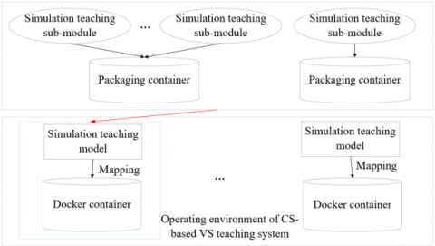
It is impossible to dynamically model the CS-based VS teaching system, without virtual packaging the simulation elements and modules on Docker. Before building the dynamic model, the mapping between the simulation elements and modules, which are related to the task, in Docker containers must be determined, such that the program can start in the shortest time and operate at the highest efficiency (Figure 4).
Figure 3. The simplified architecture of the CS-based VS teaching system
Figure 4. The mapping of dynamic model to Docker containers
The startup time and operating efficiency of the program are mainly determined by the computing power and memory allocated to program running sub-nodes and connection nodes of simulation elements, and also affected by the bandwidth and storage space allocated to each sub-module during the reception of simulation data. Therefore, the mapping of dynamic model to Docker containers was established based on five factors: processor resource allocation D271, memory resource allocation D272, bandwidth resource allocation D273, storage resource allocation D274, and task scheduling priority D275. The computing power required for the dynamic model can be quantified by:
${{C}_{DM\text{-}C}}={{\omega }_{1}}{{C}_{cpu}}+{{\omega }_{2}}{{C}_{ram}}$ (1)
where, Ccpu is processor resource allocation; Cram is memory resource allocation; ω1 and ω2 are the weight coefficients of Ccpu and Cram, respectively. The networking performance required for the dynamic model can be quantified by:
${{C}_{DM\text{-}N}}={{\omega }_{3}}{{C}_{band}}+{{\omega }_{4}}{{C}_{SS}}$ (2)
where, Cband is bandwidth resource allocation; CSS is storage resource allocation; ω3 and ω4 are the weight coefficients of Cband and CSS, respectively. Thus, the dynamic model of the CS-based VS teaching system can be expressed as:
$DM=\{{{M}_{Dyn}},{{N}_{Dyn}},R{{A}_{Dyn}},N{{P}_{Dyn}}\}$ (3)
where, MDyn={model1, model2, …, modeln} is the set of n sub-modules in the dynamic model; NDyn={Nmodeli,modelj|modeli, modeljÎNDyn} is the set of connection nodes between the sub-modules; RADyn={RAmodeli|modeliÎNDyn} is the set of computer resource configuration performance (CRCP) in the dynamic model; NPDyn={Pmodeli,modelj|modeli, modeljÎNDyn} is the set of networking performance between sub-modules. Each Docker container can be described as:
$DOCKER=\{{{D}_{Doc}},{{N}_{Doc}},R{{A}_{Doc}},N{{P}_{Doc}}\}$ (4)
where, DDoc={Doc1, Doc2, …, Docm} is the set of m Docker containers; NDoc={NDoci,Docj|Doci, DocjÎNDoc} is the set of connection nodes between the containers; RADoc={RADoci|DociÎNDoc} is the set of CRCP provided by the containers; NPDoc={PDoci,Docj|Doci, DocjÎNDoc} is the set of networking performance required between the containers. Then, the mapping map=h(model) of sub-modules in the dynamic model to the containers can be defined as:
$MAP=\{{{D}_{map}},{{I}_{R}},{{C}_{R}},{{U}_{R}}\}$ (5)
where, Dmap={modelmap1, modelmap2, …, modelmapm} is the set of containers after the deployment of sub-modules, Dmap=DDoc; Nmap={Nmodel-mapi,model-mapj|modelmapi, modelmapjÎNmap} is the set of connection nodes between the containers after the deployment of sub-modules; Nmap=NDoc;RAmap={RAmodel-mapi|modelmapiÎNmap} is the set of CRCP within container Doci as required by sub-modules; NPmap={Pmodel-mapi,model-mapj|modelmapi, modelmapjÎNmap} is the set of networking performance required for the sub-module deployed between Doci and Docj (∀Nmodel-mapi,model-mapjÎNmap, h(modelmapi)=Doci).
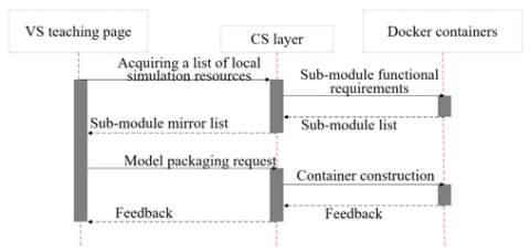
In general, the total CRCP required by the dynamic model must be smaller than the CRCP of Docker containers, and the total networking performance required by the dynamic model must be smaller than the networking performance of Docker containers. Figure 5 presents the sequence diagram of the dynamic modeling. The number of sub-modules to be deployed in the containers can be derived from the optimal mapping.
Figure 5. The sequence diagram of the dynamic model
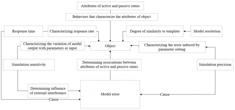
The simulation accuracy of the VS teaching system could be affected by various factors. This paper evaluates the simulation accuracy of the system from eight dimensions: object, attributes of active and passive states, associations between these attributes, model resolution, model error, simulation sensitivity, response time, and simulation precision. Figure 6 shows the evaluation model of the system simulation accuracy.
Figure 6. The accuracy evaluation model
The simulation accuracy of the dynamic model was evaluated in the following steps, according to the requirements on the CS-based VS teaching system and the eight evaluation dimensions.
(1) Verification of system requirements
The verification of system requirements aims to judge whether the CS-based VS teaching system can satisfy the user needs for simulation, and the developer needs for development, maintenance, and update, from the following four aspects: interfacing module interactions; managing developer and user configurations; environment design and program running; data collection and processing.
Let DEMU be the set of user needs for simulation, and DEMS be the set of functions realized by the system. In addition, the object and the simulation model are denoted as OU and OS, respectively; the attributes of the object and those of the simulation model are denoted as AU and AS, respectively; the associations between the attributes of the object and those of the simulation model are denoted as RU and RS, respectively. Then, DEMU and DEMS can be expressed as:
$\left\{ \begin{align} & DE{{M}_{U}}=\left\{ {{O}^{U}},{{A}^{U}},{{R}^{U}} \right\} \\ & DE{{M}_{S}}=\left\{ {{O}^{S}},{{A}^{S}},{{R}^{S}} \right\}\\\end{align} \right.$ (5)
where, ΔOU, ΔAU, and ΔRU are the deviations between the object and the simulation model. If the deviations are acceptable to the developer or user, the functions of the VS teaching system can meet the user needs for simulation.
(2) Verification of sub-module accuracy
The verification of sub-module accuracy aims to judge whether the sub-modules can satisfy the user demand for simulation accuracy from the eight dimensions. Here, the sub-module and the evaluation model for sub-module are denoted as OM and OE, respectively; the attributes of the sub-module and those of the evaluation model for sub-module are denoted as AM and AE, respectively; the associations between the attributes of the sub-module and those of the evaluation model for sub-module are denoted as RM and RE, respectively. Then, the set MSM of sub-modules and the set MSE of evaluation models for sub-module can be respectively expressed as:
$\left\{ \begin{align} & M{{S}_{M}}=\left\{ {{O}^{M}},{{A}^{M}},{{R}^{M}},\Delta E_{A}^{M},S_{A}^{M},P_{A}^{M} \right\} \\ & {{S}_{E}}=\left\{{{O}^{E}},{{A}^{E}},{{R}^{E}},\Delta E_{A}^{E},S_{A}^{E},P_{A}^{E} \right\} \\\end{align} \right. $ (7)
where, ΔEMA and ΔEEA are the set of errors of the active and passive state attributes of the sub-module accepted by the developer/user, respectively; SMA and SEA are the set of simulation sensitivities of the active and passive state attributes of the sub-module accepted by the developer/user, respectively; PMA and PEA are the set of simulation precisions of the sub-module accepted by the developer/user, respectively. Each sub-module of the VS teaching system needs to satisfy the following constraints:
$\left\{ \begin{align} & O_{L}^{M}\le {{O}^{E}}\le O_{H}^{M} \\ & A_{L}^{M}\le {{A}^{E}}\le A_{H}^{M} \\ & R_{L}^{M}\le {{R}^{E}}\le R_{H}^{M} \\ & \Delta E_{AL}^{M}\le \Delta E_{A}^{E}\le \Delta E_{H}^{M} \\ & S_{AL}^{M}\le S_{A}^{E}\le S_{H}^{M} \\ & P_{AL}^{M}\le P_{A}^{E}\le P_{H}^{M} \\\end{align} \right.$ (8)
where, OLM and OHM are the minimum and maximum of OM, respectively; ALM and AHM are the minimum and maximum of AM, respectively; RLM and RHM are the minimum and maximum of RM, respectively; ΔEALM and ΔEAHM are the minimum and maximum of ΔEAM, respectively; SALM and SAHM are the minimum and maximum of SAM, respectively; PALM and PAHM are the minimum and maximum of PAM, respectively. If a sub-module of the VS teaching system satisfies the above formula, then the sub-module meets the required simulation accuracy.
(3) Verification of simulation model accuracy
The verification of simulation model accuracy aims to judge whether the simulation model, which is made up of the sub-modules, can satisfy the user demand for simulation accuracy from the eight dimensions.
Here, the simulation model and its evaluation model are denoted as OF and OFE, respectively; the attributes of the simulation model and those of the evaluation model are denoted as AF and AFE, respectively; the associations between the attributes of the simulation model and those of the evaluation model are denoted as RF and RFE, respectively. Then, the set MSF of simulation models and the set MSFE of evaluation models can be respectively expressed as:
$\left\{ \begin{align} & M{{S}_{F}}=\left\{ {{O}^{F}},{{A}^{F}},{{R}^{F}},\Delta E_{A}^{F},S_{A}^{F},P_{A}^{F} \right\} \\ & M{{S}_{FE}}=\left\{ {{O}^{FE}},{{A}^{FE}},{{R}^{FE}},\Delta E_{A}^{FE},S_{A}^{FE},P_{A}^{FE} \right\} \\\end{align} \right. $ (9)
As can be seen from formula (9), if the deviations between the simulation model and its evaluation model are acceptable to the system developer or user, then the simulation model, which is made up of the sub-modules, passes the accuracy verification.
(4) System acceptance
Through the quantitative verifications above, the evaluators of simulation accuracy will make the final decision on the acceptance of the VS teaching system.
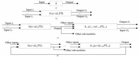
Precision is an important indicator of the reliability, credibility, and simulation accuracy of the VS teaching system. For the CS-based VS teaching system, the output of each sub-module is partially taken as the input of another VS teaching system. Considering the information transmission error between the sub-modules, it is necessary to analyze the simulation sensitivity of multiple sets of parameters in each sub-module, and evaluate how much the parameters that induce large simulation error affects the simulation model. Figure 7 provides the block diagram of the simulation accuracy analysis model for the VS teaching system.
Figure 7. The block diagram of the simulation accuracy analysis model
As shown in Figure 7(a), it is assumed that an input a of the object is simulated by model modeli, whose error is ΔEi. Then, the simulation sensitivity of modeli can be expressed as:
${{S}_{i}}=\left| {{h}_{i}}\left( a+\Delta {{E}_{i}} \right)-{{{\bar{h}}}_{i}}\left( a \right) \right|/{{\bar{h}}_{i}}\left( a \right)$ (10)
where, hi(a) is the input-output relationship of the i-th sub-module; hi(a) is the input-output relationship of the corresponding object. If the parameter settings of the sub-module have deviation, then modeli will output different results under the same input a. The object often has multiple input-output relationships, and maintains nonlinear uncertain mappings with each sub-module. Suppose IN and OM are the input and output vectors of the object, respectively, and PS is the set of sub-module parameters with simulation deviation.
As shown in Figure 7(b), it is assumed that IN contains x precise inputs. Then, the simulation sensitivity of the simulation model composed of a single sub-module can be expressed as:
$S=\left| h\left( a+\Delta E \right)-\bar{h}\left( a \right) \right|/\bar{h}\left( a \right)$ (11)
where, h(a) is the input-output relationship of the simulation model; $\bar{h}(a)$ is the input-output relationship of the corresponding object.
As shown in Figure 7(c), if the simulation model is composed of multiple sub-modules in series, the simulation sensitivity of the i-th sub-module needs to be computed by formula (11). Then, the output error hi(a+ΔEi)- $\bar{h}_{l}(a)$ of the i-th sub-module will be inputted as the error ΔEi+1 of the i+1-th sub-module.
As shown in Figure (d), if the simulation model is composed of multiple sub-modules in series, and if the errors are fed back via the coupling between these sub-modules, it is assumed that the multiple sub-modules have no simulation deviation in parameter setting and all adopt the single-input single-output mode. Then, the input and output of sub-module modeli at time t can be expressed as Iti and Oti=hi(Iti), respectively; the output of sub-module modeli+1 at time t can be expressed as Oti+1=hi+1[hi(Iti)], which is the input of sub-module modeli+2 at time t. This derivation process continues until the output of the i+k-th sub-module modeli+k is taken as the input of modeli at time t+1. Then, a new derivation process will begin. The simulation state of each sub-module can be obtained by:
$\left\{ \begin{matrix} I_{i}^{t}=O_{i+k}^{t+1},O_{i}^{t}={{h}_{i}}\left( I_{i}^{t} \right)\Delta {{E}_{i}}={{h}_{i}}\left( I_{i}^{t}+\Delta {{E}_{i+k}} \right)-{{{\bar{h}}}_{i}}\left( I_{i}^{t} \right) \\ I_{i+1}^{t}=O_{i}^{t},O_{i+1}^{t}={{h}_{i+\text{1}}}\left( I_{i+\text{1}}^{t} \right)\Delta {{E}_{i+1}}={{h}_{i+1}}\left( I_{i+1}^{t}+\Delta {{E}_{i}} \right)-{{{\bar{h}}}_{i+1}}\left( I_{i+1}^{t} \right) \\ ... \\ I_{i+k}^{t}=O_{i+k-1}^{k},O_{i+k}^{t}={{h}_{i+k}}\left( I_{i+k}^{t} \right)\Delta {{E}_{i+k}}={{h}_{i+k}}\left( I_{i+k}^{t}+\Delta {{E}_{i+k-1}} \right)-{{{\bar{h}}}_{i+k}}\left( I_{i+k}^{t} \right) \\\end{matrix} \right. $ (12)
From formulas (11)-(13), the simulation sensitivity of each sub-module and that of the overall model composed of these sub-modules can be obtained.
The CS-based VS teaching system must be able to store the important simulation data in the teaching process in a continuous manner. When the VS teaching system crashes due to software or hardware problems, the data of the continuous storage unit will be read to restore the previous system state.
In this paper, a simulation system is built upon the MySQL cloud database. The simulation data were extracted, stored, and managed through the object-relational mapping (ORM) under the Hypertext Transfer Protocol (HTTP) framework for the rapid development of Go applications. The key information is about developer and user, simulation elements, sub-modules, and mirror database. In addition, the CS-based VS platform was also constructed. Some data are listed in Tables 1-3.
As shown in Table 1, the cloud database for our VS teaching system was designed from the perspectives of ID, name, address, service structure, version, and domain. To ensure the performance of cloud mirror service, an independent storage space was allocated for the mirror data, and a mirror address was allocated by the Docker container. Furthermore, the authors also defined the types of sub-modules required for cloud simulation task, as well as the total number of parallel execution tasks that characterizes the simulation capability of the simulation system.
The proposed CS-based VS teaching system was compared with VMware, kernel-based Virtual Machine (KVM), QEMU, common language runtime (CLR) of .Net, and Docker. To ensure the accuracy of the comparison, the simulation model of three sub-modules was tested five times under each environment. The mean value of the five tests was taken as the final result under the corresponding environment.
Table 1. The cloud database of the VS teaching system
|
Type |
Format |
Size |
Null |
Description |
|
ID |
Integer |
15 |
/ |
Database function |
|
Name |
Character |
20 |
/ |
Name database |
|
Address |
Character |
26 |
/ |
Database IP address |
|
Service interface |
Integer |
20 |
/ |
Connection ports between database and other service modules |
|
Version |
Integer |
5 |
/ |
Database version |
|
Field |
Character |
5 |
/ |
Database type |
Note: ID and IP are short for identity and Internet protocol, respectively.
Table 2. The cloud mirror data
|
Type |
Format |
Size |
Invalid |
Description |
|
ID |
Integer |
15 |
/ |
Mirror function |
|
Name |
Character |
20 |
/ |
Mirror name |
|
Address |
Character |
26 |
/ |
Mirror address assigned by Docker container |
|
Size |
Integer |
15 |
/ |
Mirror data capacity |
|
Date |
Long date format |
5 |
/ |
Mirror creation time |
|
Type |
Integer |
5 |
/ |
Mirror type |
|
Class |
Integer |
5 |
/ |
Mirror tool, federal class |
|
Storage space |
Character |
15 |
/ |
Mirror data storage space |
Table 3. The data on cloud simulation task
|
Type |
Format |
Size |
Null |
Description |
|
ID |
Integer |
15 |
/ |
Task function |
|
Name |
Character |
20 |
/ |
Task name |
|
Number of tasks |
Integer |
10 |
/ |
Number of tasks |
|
Creation time |
Long date format |
5 |
/ |
Task creation time |
|
Execution time |
Long date format |
20 |
/ |
Task execution time |
|
Type |
Integer |
5 |
/ |
Task type |
|
Class |
Integer |
5 |
/ |
Task module class |
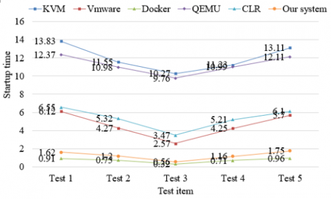
Figure 8 compares the startup time under different frameworks. Obviously, the startup time of the simulation program varied significantly between environments. The startup time under KVM and QEMU was 12-14 times that under Docker. The proposed system consumed a relatively short time to start up, only slightly longer than the startup time under Docker. But our system is simple and efficient, as it maps the dynamic model into Docker containers. The high simplicity and efficiency offset the slightly longer startup time.
Figure 8. The comparison of startup time
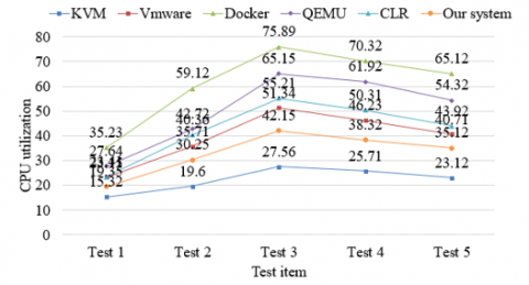
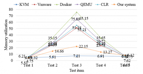
In addition, a simple first-order automatic control system was simulated under the above environments in the presence of disturbance. Figures 9 and 10 compares the CPU utilization and memory utilization under different environments. It can be seen that the system did not consume much CPU or memory resources under the proposed CS-based VS teaching platform, while facilitating the management and execution of simulation resources and sub-modules.
Figure 9. The comparison of CPU utilization
Note: CPU is short for central processing unit.
Figure 10. The comparison of memory utilization
This paper designs an innovative CS-based VS teaching system. Firstly, the functional requirements on the CS-based VS teaching system were analyzed, and decomposed into such three layers as goal, function type, and function name. On this basis, a dynamic model was established for the CS-based VS teaching system. The simulation accuracy and precision of the model were verified in multiple dimensions. To verify the performance of the proposed system, a simulation system was built upon the MySQL cloud database, the simulation data were extracted, stored, and managed through ORM under the HTTP framework for the rapid development of Go applications, and the CS-based VS teaching platform was constructed. The experimental results confirm that the proposed system not only boasts good simulation performance, but also enjoys advantages in simplicity and efficiency, owing to the mapping of the dynamic model to Docker containers. The startup time, CPU utilization, and memory utilization of our system were all controlled at low levels. The research results provide a reference for the application of CS-based system design in other fields.
[1] Kim, J.W., Choi, J.W., Lee, I.W. (2016). Design and simulation of an optimal microgrid system. 2016 International Conference on Information and Communication Technology Convergence (ICTC), Jeju, pp. 1061-1064. https://doi.org/10.1109/ICTC.2016.7763368
[2] Zeraatkar, N., Farahani, M.H., Rahmim, A., Sarkar, S., Ay, M.R. (2016). Design and assessment of a novel SPECT system for desktop open-gantry imaging of small animals: A simulation study. Medical Physics, 43(5): 2581-2597. https://doi.org/10.1118/1.4947127
[3] Baghli, F.Z., El Bakkali, L. (2016). Design and simulation of robot manipulator position control system based on adaptive fuzzy PID controller. Robotics and Mechatronics, 243-250. https://doi.org/10.1007/978-3-319-22368-1_24
[4] Alavinia, R., Zhu, Z., Zhang, S. (2016). Design and simulation of a meteorological data monitoring system based on a wireless sensor. International Journal of Online and Biomedical Engineering (iJOE), 12(5): 27-32. http://dx.doi.org/10.3991/ijoe.v12i05.5733
[5] Mahmoud, A.E., Mahmoud, O.E., Fatouh, M. (2016). Development of design optimized simulation tool for water desalination system. Desalination, 398: 157-164. https://doi.org/10.1016/j.desal.2016.07.022
[6] Singh, A., Ramesh, M.V., Divya, P. (2016). Design and simulation of elephant intrusion detection system. 2016 6th International Workshop on Computer Science and Engineering, WCSE, Tokyo, Japan, pp. 749-753.
[7] El-Nemr, M.K., Omara, A.M. (2016). Design and simulation of a battery powered electric vehicle implementing two different propulsion system configurations. 2016 Eighteenth International Middle East Power Systems Conference (MEPCON), Cairo, pp. 877-882. https://doi.org/10.1109/MEPCON.2016.7836999
[8] Ijagbemi, C.O., Oladapo, B.I., Campbell, H.M., Ijagbemi, C.O. (2016). Design and simulation of fatigue analysis for a vehicle suspension system (VSS) and its effect on global warming. Procedia Engineering, 159: 124-132. https://doi.org/10.1016/j.proeng.2016.08.135
[9] Ekinci, S., Demirören, A. (2016). Modeling, simulation, and optimal design of power system stabilizers using ABC algorithm. Turkish Journal of Electrical Engineering & Computer Sciences, 24(3): 1532-1546.
[10] Jeong, S., Lee, M.S., Cho, K., Jang, Y.J. (2016). System model and simulation for optimal parameter design of dynamic wireless charging EVs. 2016 IEEE Transportation Electrification Conference and Expo, Asia-Pacific (ITEC Asia-Pacific), Busan, pp. 082-089. https://doi.org/10.1109/ITEC-AP.2016.7512927
[11] Hong, J.H., Ryu, K.R. (2017). Simulation-based multimodal optimization of decoy system design using an archived noise-tolerant genetic algorithm. Engineering Applications of Artificial Intelligence, 65: 230-239. https://doi.org/10.1016/j.engappai.2017.07.026
[12] Modaresi, A., Safikhani, A., Noohi, A.M.S., Hamidnezhad, N., Maki, S.M. (2017). Gating system design and simulation of gray iron casting to eliminate oxide layers caused by turbulence. International Journal of Metalcasting, 11(2): 328-339. https://doi.org/10.1007/s40962-016-0061-3
[13] Liu, W., Liu, S. (2017). Design of medical track logistics transmission and simulation system based on internet of things. Acta Technica, 62(1): 207-220.
[14] Cheshmehbeigi, H.M., Khanmohamadian, A. (2017). Design and simulation of a moving-magnet-type linear synchronous motor for electromagnetic launch system. International Journal of Engineering, 30(3): 351-356.
[15] Avital, E.J., Salvatore, E., Munjiza, A., Suponitsky, V., Plant, D., Laberge, M. (2017). Flow design and simulation of a gas compression system for hydrogen fusion energy production. Fluid Dynamics Research, 49(4): 045504. https://doi.org/10.1088/1873-7005/aa73ba
[16] Aguilar-Gonzalez, A., Nolazco-Flores, J.A., Vargas-Rosales, C., Bustos, R. (2017). Characterisation, design and simulation of an efficient peer-to-peer content distribution system for enterprise networks. Peer-to-Peer Networking and Applications, 10(1): 122-137. https://doi.org/10.1007/s12083-015-0412-5
[17] Hashemipour, M., Stuban, S., Dever, J. (2018). A disaster multiagent coordination simulation system to evaluate the design of a first-response team. Systems Engineering, 21(4): 322-344. https://doi.org/10.1002/sys.21437
[18] Savastru, D., Miclos, S., Savastru, R., Lancranjan, I. (2018). Simulation and design of a LPGFS system for detection of Escherichia coli bacteria infestation in milk. Journal of Optoelectronics and Advanced Materials, 610-617.
[19] Nasri, F., Alqurashi, F., Nciri, R., Ali, C. (2018). Design and simulation of a novel solar air-conditioning system coupled with solar chimney. Sustainable Cities and Society, 40: 667-676. https://doi.org/10.1016/j.scs.2018.04.012
[20] Schaefer, R., Wesuls, J.H., Köckritz, O., Korte, H., Windeck, K.J. (2018). A mobile manoeuvring simulation system for design, verification and validation of marine automation systems. IFAC-PapersOnLine, 51(29): 195-200. https://doi.org/10.1016/j.ifacol.2018.09.492
[21] Bajpai, A., Ghasemi, M., Song, X. (2019). Design and simulation of a lab-scale down-hole drilling system. Proceedings of the Institution of Mechanical Engineers, Part C: Journal of Mechanical Engineering Science, 233(8): 2591-2598. https://doi.org/10.1177/0954406218797978
[22] Loukriz, A., Messalti, S., Harrag, A. (2019). Design, simulation, and hardware implementation of novel optimum operating point tracker of PV system using adaptive step size. The International Journal of Advanced Manufacturing Technology, 101(5-8): 1671-1680. https://doi.org/10.1007/s00170-018-2977-7
[23] Maeda, M., Furutaka, K., Kureta, M., Ohzu, A., Komeda, M., Toh, Y. (2019). Simulation study on the design of nondestructive measurement system using fast neutron direct interrogation method to nuclear materials in fuel debris. Journal of Nuclear Science and Technology, 56(7): 617-628. https://doi.org/10.1080/00223131.2019.1611500
[24] Ghosh, A., Jain, A., Sarkar, S.K. (2019). Design and simulation of nanoelectronic data transfer system with an emphasis on reliability and stability analysis. Analog Integrated Circuits and Signal Processing, 101(1): 13-21. https://doi.org/10.1007/s10470-018-01384-9
[25] Ferraresi, C., De Benedictis, C., Maffiodo, D., Franco, W., Messere, A., Pertusio, R., Roatta, S. (2019). Design and simulation of a novel pneumotronic system aimed to the investigation of vascular phenomena induced by limb compression. Journal of Bionic Engineering, 16(3): 550-562. https://doi.org/10.1007/s42235-019-0045-0