Taha Hocine Kerbaa | Amar Mezache | Houcine Oudira*
© 2020 IIETA. This article is published by IIETA and is licensed under the CC BY 4.0 license (http://creativecommons.org/licenses/by/4.0/).
OPEN ACCESS
In a previous work, it has been shown that the application of a modified fractional order moment (MFOM) estimator leads to the same accuracy as the [zlog(z)] method with lower computation complexity. However, undesirable estimation performances have been observed for single look data, low sample sizes and large values of the K-distribution shape parameter. Moreover, the application of positive and negative order moments estimators (PNOME) has a serious impact on the estimation accuracy of the shape parameter. To reduce this sensitivity, it is important to apply thresholding approaches in the case of a single pulse transmission. To this effect, single and double thresholding estimators are proposed in this paper and the Otsu’s algorithm is used to compute underlying thresholds. On the basis of Monte-Carlo simulation, the performances of the proposed estimators are assessed against moments and [zlog(z)] methods. Experiment examples indicate that the thresholding approaches based on the Otsu’s algorithm is more accurate with computational advantages than existing estimators.
K-clutter plus noise, parameter estimation, fractional order moments, thresholding, Otsu’s algorithm
Radar clutter echoes consist of radar returns from reflectors that are not of interest and often obscure the signals from targets that are of interest. With the advent of high resolution radars, modelling of sea clutter has attracted the attention of researchers from various fields for decades. It is well known that the Gaussian model of low-resolution complex backscatter has reached its limit in understanding the strong spiky returns from ocean waves in high-resolution radar at low grazing angles [1, 2]. Performances of detection and tracking radar targets in homogeneous and heterogeneous environments are highly dependent on the selected clutter model. That is why, in real life applications, we often seek for adequate distributions in terms of radar parameters and background’s statistics. To this end, several types of clutter distributions inspired from the generalized compound model have been proposed [3]. The first works on sea clutter modelling show that two parameters log-normal, Weibull, K, Pareto type 2, K-LNT (K log-normal texture) and CG-IG (compound Gaussian Invers Gaussian) models have been proposed to generally fit empirical non-Gaussian clutter. However, thermal system noise and Rayleigh clutter may appear as additive quantities to randomly clutter intensities where above models are extended to incorporate Gaussian noise [2, 4]. These mixture models having three parameters are given in integral forms which complicate the development of parameter estimation and target detection schemes.
Estimation of K plus noise distribution parameters has been discussed and some interesting approaches with different degrees of accuracies are proposed in literatures [4-9]. The high order moment estimator (HOME) is obtained as a function of the first three intensity moments and involves very large data samples [4]. Parametric curve fitting estimator (PCFE) proposed in reference [5] provides shape parameter values after the optimization of residuals among theoretical and real CCDFs (Complementary Cumulative Distributed Functions). This method is used to any kind of radar clutter model with or without thermal noise. Bocquet [6] derived two estimation approaches; the [zlog(z)] method depending on the generalized exponential integral function and the constrained maximum log likelihood estimator (CMLE) method. Using moments of order 1 and 2, fractional order moments (FOME) and [zlog(z)] approaches are derived in references [7, 8] in terms of the hypergeometric functions. Regarding their heavy computational load, these methods achieve accurate estimates against HOME and PCFE methods. Recently, the employment of two statistical ratios in reference [9] eliminates in fact the hypergeometric functions given in reference [7]. More precisely, from references [7, 8], the problem of the shape parameter estimation was the complexity of numerical computations of the hypergeometric functions. The latters are eliminated after the manipulation of two statistical ratios with a recurrence relation of the hypergeometric functions [9]. The resulting estimators are executed in terms of clutter statistics and fractional moment order without hypergemetric functions. Parameter estimation for a compound radar clutter model with trimodal discrete texture is proposed and yield a fairly good description of experimental data [10].
Compared with the [zlog(z)] method given in reference [8], it is observed that the modified FOME (MFOME) given in reference [9] method provides similar results for multi-look case. However, the latter does not exhibit its effectiveness for cases of single look data, low sample sizes and large values of the shape parameter. In the intensity domain, the form of the K-clutter plus noise distribution is conventionally given by
$p\left( z \right)=\int\limits_{0}^{\infty }{{{p}_{\left. z \right|y}}\left( \left. z \right|y,N \right)}{{p}_{y}}\left( y \right)dy$ (1)
where, Z is the intensity variable, y is the modulation component with a density function py(y), and z|y is the speckle component with a conditional pdf pz|y (z|y, N). We denote the thermal noise power by 2σ2=pn and assume that the returns from N successive pulses are uncorrelated. Random variables Z|Y and Y follow gamma distributions with shape parameters N and v respectively
$\left\{ \begin{align} & {{p}_{\left. Z \right|Y}}\left( \left. z \right|y \right)=\frac{{{z}^{N-1}}}{{{(y+{{p}_{n}})}^{N}}\Gamma \left( N \right)}\exp \left( -\frac{z}{y+{{p}_{n}}} \right) \\ & p(y)=\frac{{{b}^{\nu }}{{y}^{\nu -1}}}{\Gamma (\nu )}\exp \,(-by) \\\end{align} \right.$ (2)
where, Γ(.) is the gamma function and b the scale parameter. Substituting Eq. (2) into Eq. (1), the K clutter plus noise model is given by [4, 5]
${{p}_{Z}}\left( z \right)\text{ }=\frac{{{b}^{\nu }}{{z}^{N-1}}}{\Gamma (N)\,\Gamma \left( \nu \right)}\int\limits_{0}^{\infty }{\frac{{{y}^{\nu -1}}}{{{({{p}_{n}}+y)}^{N}}}\exp \,\,\left( -\frac{z}{{{p}_{n}}+y}-by \right)\,dy}\text{ }$ (3)
From Eq. (3), moments of order p are given by
$\langle {{Z}^{p}}\rangle =\frac{{{b}^{\nu }}\text{ }\Gamma (p+N)}{\Gamma (N)\text{ }\Gamma (\nu )}\int\limits_{0}^{\infty }{{{({{p}_{n}}+y)}^{p}}}{{y}^{\nu \text{-1}}}\exp \,(-b\text{ }y)\text{ }dy$ (4)
where, $\langle .\rangle $ denotes expectation.
Remarkable estimation errors are perceived for cases of single look data, low sample sizes and large values of the K-distributed shape parameter [9]. In addition, the application of positive and negative order moments provides different degrees of estimation accuracy. Thereby, it is interesting to apply thresholding approaches for a single look data. To this end, single and double thresholding estimators are proposed here and the Otsu’s algorithm is used to compute underlying thresholds. Through simulated data, estimation performances are compared with existing HOME, MFOME and [zlog(z)] approaches. It is shown that small estimation errors are obtained by the proposed thresholding approaches with low computational complexity. The main contribution of this work is the improvements of the shape parameter estimates through the combination of estimators given by Sahed and Mezache [9] and thresholding techniques based on the Otsu’s algorithm.
The remaining part of the paper is organized as follows. Summary of existing estimators of K-clutter plus noise parameter is presented in Section 2. The proposed thresholding estimators are given in Section 3. Estimation results of single and double thresholding methods are compared with those given by HOME and [zlog(z)] approaches in Section 4. Finally, conclusions are reported in Section 5.
Before describing estimators of K-clutter plus noise parameters using thresholding approaches, we will summarize in this section relevant estimators based on integer moments, fractional order moments and log moments.
2.1 HOME method
The HOME method suggests that Eq. (4) can be solved in a closed form for integer values of p [4]. That is, by solving the integrals for p=1, 2 and 3, the estimate of the shape parameter is
$\hat{\nu }=\frac{18\,\,{{({{{\hat{\mu }}}_{2}}-2{{{\hat{\mu }}}_{1}}^{2})}^{3}}}{{{(12{{{\hat{\mu }}}_{1}}^{3}-9{{{\hat{\mu }}}_{1}}{{{\hat{\mu }}}_{2}}+{{{\hat{\mu }}}_{3}})}^{2}}}$ (5)
where, the sample moment $\hat{\mu}_{p}$ of order p is computed from M independent and identically distributed (iid) samples of the intensity variable Z,
${{\hat{\mu }}_{p}}=\langle Z{{\,}^{p}}\rangle =\frac{1}{M}\sum\limits_{i=1}^{M}{z_{i}^{p}}\text{ }$ (6)
$\hat{p}_{n}$ and $\widehat{b}$ are expressed in terms of $\hat{v}$ and the first two moments.
$\left\{ \begin{align} & {{{\hat{p}}}_{n}}={{{\hat{\mu }}}_{1}}-{{(0.5\hat{\nu }\,({{{\hat{\mu }}}_{2}}-2{{{\hat{\mu }}}_{1}}^{2}))}^{1/2}} \\ & \hat{b}=\frac{{\hat{\nu }}}{{{{\hat{\mu }}}_{1}}-{{{\hat{p}}}_{n}}} \\\end{align} \right.$ (7)
The performance of HOME method decreases for low sample sizes and low clutter-to-noise ratio (CNR=v/bpn) [5].
2.2 FOME method
When p is fractional, moments given by Eq. (4) are solved in terms of the confluent hypergeometric function, $_{2}{{F}_{0}}\left( .;.;. \right)$ [7]. Hence
${{\mu }_{p}}=\frac{p_{n}^{\alpha }\Gamma \left( p+N \right)}{\Gamma \left( N \right)}{{\text{ }}_{\text{2}}}{{F}_{0}}\left( \nu ,-p;.;-1/b{{p}_{n}} \right)$ (8)
The effective shape parameter, $v_{\mathrm{eff}}=\frac{(N+1)\langle z\rangle^{2}}{N\left\langle z^{2}\right\rangle-(N+1)\langle z\rangle^{2}}$ is substituted into Eq. (8) in order to reduce the estimation problem in one dimension. Thus, Eq. (8) becomes
$\frac{{{{\hat{\mu }}}_{p}}\,{{N}^{p}}\,\Gamma \left( N \right)}{{{{\hat{\mu }}}^{p}}\,\Gamma \left( N+p \right)}={{\left( 1-\sqrt{\frac{{\hat{\nu }}}{{{\nu }_{eff}}}} \right)}^{p}}_{\text{2}}{{F}_{0}}\left( \hat{\nu },-p;.;-{{\left( \sqrt{\hat{\nu }{{\nu }_{eff}}}-\hat{\nu } \right)}^{-1}} \right)$ (9)
After calculating $\hat{\mu}$ and $\hat{\mu}_{p}$ from the data, Eq. (9) is solved numerically and offers better results with respect to the HOME method. Nevertheless, it is noticed that the performance of that estimator varies due to numerical computations errors of $_{2}{{F}_{0}}\left( .;.;. \right)$ with significant execution time.
2.3 [zlog(z)] method
In [zlog(z)] estimator, log moments denoted by log(Z), ⟨log(Z)⟩ and Zlog(Z) are employed and the estimates are given in terms of $_{2}{{F}_{0}}\left( .;.;. \right)$ [8]
$\frac{\langle Z\log (Z)\rangle \text{ }}{\langle Z\rangle }-\langle \log (Z)\rangle =\text{ }\frac{1}{N}+\frac{1-{{\text{ }}_{\text{2}}}{{F}_{0}}(\hat{\nu },1;.;-{{(\sqrt{\hat{\nu }{{\nu }_{\text{eff}}}}-\hat{\nu })}^{-1}})}{\sqrt{\hat{\nu }{{\nu }_{\text{eff}}}}}$ (10)
If N>1, Eq. (8) and Eq. (9) are handled to determine a closed form of [zlog(z)] estimator in terms of the inverse harmonic mean denoted by <Z-1> given by
$\hat{\nu }={{\nu }_{\text{eff}}}{{\left( \frac{1-\frac{N-1}{N}\langle Z\rangle \langle {{Z}^{-1}}\rangle }{{{\nu }_{\text{eff}}}\left( \frac{\langle Z\log (Z)\rangle }{\langle Z\rangle }-\langle \log (Z)\rangle -\frac{1}{N} \right)-\frac{N-1}{N}\langle Z\rangle \langle {{Z}^{-1}}\rangle } \right)}^{2}}$ (11)
where, ⟨Z⟩, ⟨log(Z)⟩ and ⟨Zlog(Z)⟩ are calculated first from the data and straightforward computations are carried out to get $\hat{\nu }$.
2.4 MFOME method
For a single look case, recent work presented by Sahed and Mezache [9] suggested that closed form estimators of FOME method can be obtained after manipulating the following statistical ratios.
$\left\{ \begin{align} & {{\alpha }_{p,q}}=\frac{{{\mu }_{p+q}}}{{{\mu }_{p}}{{\mu }_{q}}} \\ & {{\beta }_{p,q}}=\frac{{{\mu }_{p-q}}{{\mu }_{q}}}{{{\mu }_{p}}} \\\end{align} \right.$ (12)
where, p is a positive real and q is an integer. Substituting Eq. (8) into Eq. (12) with q=1, Eq. (12) becomes.
${{\alpha }_{p,1}}=\frac{N+p}{N}\frac{\sqrt{v{{v}_{eff}}}-v}{\sqrt{v{{v}_{eff}}}}\frac{U(v,v+p+2;\sqrt{v{{v}_{eff}}}-v)}{U(v,v+p+1;\sqrt{v{{v}_{eff}}}-v)}$ (13)
and
${{\beta }_{p,q}}=\frac{N}{N+p-1}\frac{\sqrt{v{{v}_{eff}}}}{\sqrt{v{{v}_{eff}}}-v}\frac{U(v,v+p;\sqrt{v{{v}_{eff}}}-v)}{U(v,v+p+1;\sqrt{v{{v}_{eff}}}-v)}$ (14)
where, $U(.,.;.)$ is the Tricomi or the confluent hypergeometric function. Using the recurrence relation U(a,b+1,z)=(b-1+z)U(a,b,z)+(a-b+1)U(a,b-1,z) given by Sahed and Mezache [9], it can be seen by replacing, a=v, b=v+p+1 and $z=\sqrt{\nu {{\nu }_{eff}}-\nu }$ that
$\hat{\nu }={{\nu }_{eff}}{{\left( \frac{1-\frac{N+p-1}{N}{{{\hat{\beta }}}_{p,1}}}{\frac{{{\nu }_{eff}}}{p}\left( \frac{N}{N+p}{{{\hat{\alpha }}}_{p,1}}-1 \right)-\frac{N+p-1}{N}{{{\hat{\beta }}}_{p,1}}} \right)}^{2}}$, $N \geq 1$ (15)
For N=1 and large sample sizes, the MFOME method given by Eq. (15) provides in fact computational advantages compared with numerical FOME and [zlog(z)] approaches. However, the performance of MFOME method degrades against the numerical [zlog(z)] method for both high values of v (i.e., v>0.4) and low values of M (M<2000). The question is, can one improve the estimation results for low sample sizes and high values of v with a small processing time. The next section explains how this is possible.
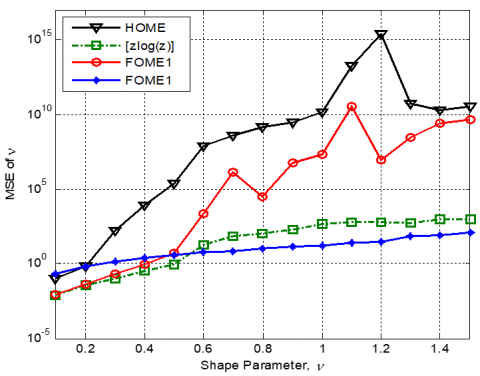
Under the hypotheses of low sample sizes and single pulsed waveform operation, it is discussed above that the MFOME discussed by Sahed and Mezache [9] is simplest and fastest to compute, but it provides poor results for high values of the shape parameter (v>0.4) with p>0”. On the other hand, if we consider a negative value of p (p=-0.5), best estimates are achieved for v>0.6 compared with [zlog(z)] approach as shown in Figure 1. Using the MFOME method, either negative or positive value of the fractional order affects absolutely the estimation precision. To maintain good estimation performance along the selected interval of the shape parameter, application of an estimation procedure that switches based on the Mean Square Errors (MSE) to the modified FOME method with p=0.5 denoted by FOME1 or the modified FOME method with p=-0.5 denoted by FOME2 is desirable. Such switching scheme is equivalent to the application of one or more preselected thresholds. For this purpose, two thresholding approaches are proposed in this work for accurate estimates of K-clutter plus noise parameters.
Figure 1. MSE of v estimates of the K-clutter plus thermal noise distribution for M =1000, N =1, CNR =0dB
3.1 Estimation using single threshold
With different values of CNR, the best choice between FOME1 and FOME2 methods that provides good estimation performance in a given range of v can be seen as a thresholding problem. Our first idea to resolve this estimation issue encountered [9] would be the use of one threshold, T that allows automatic selection among the two estimators. A single threshold based estimation method necessitates an a priori knowledge of T where a systematic approach for finding the optimal value of T that exhibits better estimation results are recommended. The maximum variance between clusters method also known as the Otsu method [11] used in image processing domain is classified as an effective thresholding technique for image segmentation. It is an exhaustive algorithm of searching the global optimal threshold T between two hypotheses (classes) H0 and H1, based on a discriminate criterion aiming at maximizing the separability between the two classes and thus minimizing their intraclass variance. Otsu method is applied in a wide range of domains. A fast region-based detection model was developed using generalized likelihood ratio test (GLRT) and Otsu thresholding technique to improve oil spill detection accuracy in Synthetic Aperture Radar (SAR) images [12]. In radar target detection application, a Constant False Alarm Rate (CFAR) algorithm based upon modified Otsu technique is proposed and resulting detection performances are analysed by Messina et al. [13]. The Otsu algorithm was also used for finding a threshold between the outputs of a deep neural network which represent, during the training phase, the values used to indicate the presence or the absence of an object [14]. In our case, the two classes represent FOME1 and FOME2 methods which give the first estimate of v (i.e., ${{\hat{\nu }}_{1}}$) and the second estimate of v (i.e., ${{\hat{\nu }}_{2}}$) respectively. Let fi(X) be the output function of the shape parameter values of ${{\hat{\nu }}_{1}}$ and ${{\hat{\nu }}_{2}}$ represented by a 1-D histogram composed of M bins. This last is transformed by normalization into a probability function p(fi(X)). Let us suppose that along fi(X) just two classes lie; namely H0 and H1. We are interested in finding a threshold value T that best separate the two classes. For a given threshold T, the prior probabilities of H0 and H1 can be computed as follows:
$\left\{ \begin{align} & P({{H}_{0}}(T))=\sum\limits_{i=0}^{t-1}{p(i)} \\ & P({{H}_{1}}(T))=\sum\limits_{i=0}^{M-1}{p(i)} \\\end{align} \right.$ (16)
The main idea behind the Otsu’s method is to pick out the threshold T that minimizes the intraclass variance of the two classes, which is none other than the weighted sum of variances of each cluster defined as:
$\sigma _{w}^{2}(T)=P({{H}_{0}}(T))\sigma _{0}^{2}+P({{H}_{1}}(T))\sigma _{1}^{2}$ (17)
where, $\sigma_{1}^{2}$ and $\sigma_{0}^{2}$ are the variance of pixels above and below the threshold T respectively, thus an approximation of the variance of the classes H0 and H1. Alternatively, we may express the minimization process in terms of the between-class $\sigma_{B}^{2}(T)$ variance, which is defined as the substraction of the within-class variance $\sigma_{w}^{2}(T)$ from the total variance of their combined distribution given by:
$\begin{align} & \sigma _{B}^{2}(T)={{\sigma }^{2}}-\sigma _{w}^{2}(T) \\ & \text{ }=P({{H}_{0}}(T)){{\left( {{\mu }_{0}}(T)-{{\mu }_{T}} \right)}^{2}}+P({{H}_{1}}(T)){{\left( {{\mu }_{1}}(T)-{{\mu }_{T}} \right)}^{2}} \\\end{align}$ (18)
where, the class means are
${{\mu }_{0}}(T)=\sum\limits_{i=0}^{T-1}{ip(i)/P({{H}_{0}})}$ (19)
and
${{\mu }_{1}}(T)=\sum\limits_{i=T-1}^{M-1}{ip(i)/P({{H}_{1}})}$ (20)
The best threshold T that minimizes the within-classes variance $\sigma_{w}^{2}(T)$ is selected as
$T=\underset{0\le t\le M-1}{\mathop{\max }}\,\sigma _{B}^{2}(T)$ (21)
For every bin T (candidate value for the best threshold) of the histogram, we thus compute the between-classes variance $\sigma_{B}^{2}(T)$ and we choose the optimum threshold T that maximizes it. This process is repeated for each output fi(X) of the vector containing values of $\hat{v}_{1}$ and $\hat{v}_{2}$.
Based on several values of CNR and v, the search for optimality is carried out off-line by the Otsu algorithm. Related steps found by Otsu [11] are used here to calculate T from $\hat{v}_{1}$ and $\hat{v}_{2}$:
Step 1: - Generate single look K-clutter plus noise data.
$z=\exp rnd\left( \left( {{p}_{n}}+gamrnd\,(\nu ,1/b,n,M \right) \right)$
where ‘exprnd’ and ‘gamrnd’ are Matlab routines used
for generation of random variables according to
exponential and gamma laws respectively.
- Calculate ${{\nu }_{eff}}$, ${{\alpha }_{p,1}}$ and $\nu \in $ from a set of the
data $\left\{ {{\text{z}}_{\text{1}}}\text{, }{{\text{z}}_{\text{2}}}\text{, }\ldots \text{, }{{\text{z}}_{\text{M}}} \right\}$ .
Step 2: - Set p = 0.5 and use (15) to calculate the 1st value of $\hat{\nu }$ denoted by ${{\hat{\nu }}_{1}}$
Step 3: - Set p = -0.5 and recalculate the 2nd value of $\hat{v}$ denoted by ${{\hat{\nu }}_{2}}$
Step 4: - Create a vector in terms of ${{\hat{\nu }}_{1}}$ and ${{\hat{\nu }}_{2}}$, i.e.,
V = [ ${{\hat{\nu }}_{1}}$ , ${{\hat{\nu }}_{2}}$ ]
- Create (nxm) matrix M from V (Input of the segmentation process)
- Normalize (rescale) min/max values of V to 0/255 which represent the 256 intensity level of a pixel in the image matrix.
Step 5: - Generate the histogram, H=hist(M,[0:255]), where ‘hist’ is the Matlab routine which returns the distribution of M among bins with center specified by the vector [0:255].
Step 6: - Calculate the mean, within-class variance and between-class variance.
Step 7: - Calculate the best threshold $\widehat{T}$ that minimizes the within-classes variance (Normalized threshold).
Step 8: - Calculate the real value of the threshold, T=[255* $\widehat{T}$ ]/max(V).
The above steps are repeated for different values of CNR and v in order to compute the threshold T for the best separation of the two estimators. Different threshold estimates are obtained and the mean value of these estimates is performed to obtain the adequate value of T. The proposed single thresholding estimator is executed using the following steps:
Step 1: - Generate single look K-clutter+noise data.
$z=\exp rnd\left( \left( {{p}_{n}}+gamrnd\,(\nu ,1/b,n,M \right) \right)$
- Calculate ${{\nu }_{eff}}$ , ${{\alpha }_{p,1}}$ and ${{\beta }_{p,1}}$ from a set of the
data $\left\{Z_{1}, \mathrm{Z}_{2}, \ldots, \mathrm{Z}_{M}\right\}$ .
Step 2: - Set p = 0.5 and use (15) to calculate ${{\hat{\nu }}_{1}}$
Step 3: - Set p = -0.5 and recalculate ${{\hat{\nu }}_{2}}$ using Eq. (15)
- Use T found by the Otsu’s method to compute $\hat{\nu }$.
if ${{\hat{\nu }}_{1}}$ < T,
$\hat{v}=\hat{v}_{1}$
else
$\hat{v}=\hat{v}_{2}$
Step 4: - According to Eq. (7), calculate $\hat{b}, \hat{p}_{n}$ and $C \widehat{N} R=\hat{v} / \hat{b} \hat{p}_{n}$.
3.2 Estimation using double threshold
With the aim of obtaining improved estimation results, switching procedure between FOME1 and FOME2 given above can also be extended by the employment of two thresholds T1 and T2 for diverse values of v and CNR. The same functionality is considered as before, but the major difference is to choose $\hat{\boldsymbol{v}}$ as the minimum value between $\hat{v}_{1}$ and $\hat{v}_{2}$ (i.e., $\hat{v}=\min \left(\hat{v}_{1}, \hat{v}_{2}\right)$ if $\hat{v}_{1} \in\left[T_{1}, T_{2}\right]$) where the min and the max values of threshold estimates given by the Otsu algorithm are used to compute T1 and T2 respectively. Estimation based on the double thresholding approach is given by the following steps:
Step 1: - Generate iid K-clutter+noise data,
{Z1, Z2, …, ZM}
- Calculate veff, αp,1 and βp,1.
Step 2: - Calculate ${{\hat{\nu }}_{1}}$ and ${{\hat{\nu }}_{2}}$ using Eq. (15).
Step 3: - Use T1 and T2 found by the Otsu’s method to
compute $\hat{\nu }$.
if ${{\hat{\nu }}_{1}}$ < T1,
$\hat{v}={{\hat{\nu }}_{1}}$
if ${{\hat{\nu }}_{1}}$ > T2,
$E[{{(\hat{\nu }-E[\hat{\nu }])}^{2}}]$
if ( ${{\hat{\nu }}_{1}}$ > T1) and ( ${{\hat{\nu }}_{1}}$ < T2)
$\hat{v}=\min ({{\hat{\nu }}_{1}},{{\hat{\nu }}_{2}})$
Step 4: - Use Eq. (7) to calculate $\hat{b}$ , ${{\hat{p}}_{n}}$ and $C\hat{N}R=\hat{\nu }/\hat{b}{{\hat{p}}_{n}}$ .
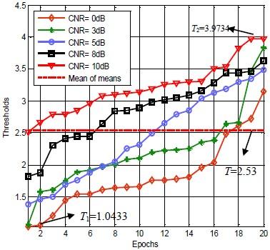
With regard to the proposed thresholding estimation methods described earlier, we proceed in this section to carry out computer simulations to assess their performances and to confirm their applicability. To this effect, we compare the estimation performance obtained by the proposed estimators against existing HOME, modified FOME and [zlog(z)] methods. The bias, the variance and the MSE metric tests are used to judge the estimation accuracy of the K-clutter plus noise shape parameter. For a single look data, the reference window’s length is set to M=700, M=1000 and 2000. K-clutter plus thermal noise samples are generated for a range [0.1-1.5] of v with different values of the CNR. In all simulations, estimates of v are averaged over n=1000 independent trails. As described in Section 3, the use of the proposed thresholding estimators requires values of T, T1 and T2. For this, the Otsu’s algorithm steps given in Section 3 are executed to compute corresponding thresholds. Because, the shape parameter estimates are related to v and CNR variables (i.e., $v \in[0.1 \quad 1.5]$)and CNR ( $C N R \in[0 d B 10 d B]$). Because, the shape parameter estimates are related to v and CNR variables, the single threshold T=2.5352 is obtained by the mean of means of threshold estimates. More precisely, for each combination of v and CNR, the mean of $\hat{{V}}$ which represents T is determined firstly from n=1000 Monte-Carlo repetitions. After that, the resulting estimates of T from all combinations are averaged to get the final value of T. Then, the minimum of means and the maximum of means are used to select values of T1 and T2 respectively as depicted from Figure 2 (T1 = 1.0433 and T2 = 3.9734).
Figure 2. Sorted threshold’s means for $v \in[0.1-1.5]$ and different CNR values and 20 trials
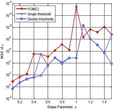
For different values of v and CNR, subsequent experiments deal with the analysis of estimation performances of the proposed switching approaches. For comparison purposes, we conduct bias and variance of different estimation methods as shown in Tables 1 and 2. For instance, we simulate K-clutter plus noise data for v =0.1, 0.5, 1 and 1.5, M = 1000, N = 1 and three values of CNR (0, 5 and 10 dB). For v =0.1, the obtained results clearly show that the single and double thresholds techniques offer accurate estimates than the FOME1 (p=0.5) with all CNR values. Moreover, with $\boldsymbol{v} \in$[0.5, 1.5], CNR=0 and CNR=5dB, Otsu’s based approaches exhibit best bias estimation performances compared with the FOME2 (p=-0.5) method which is more accurate than the FOME1 method. Roughly speaking, we emphasize that the single threshold method provides the best bias estimation performances compared with existing estimation methods. For CNR=0dB and M=1000, Figure 3 illustrates resulting MSE values of $\hat{{V}}$ . An horizontal look at this figure shows that the FOME2 method with p = -0.5 outcomes the worst results in terms of low values of v and an overlap of the FOME1 with p=0.5, single and double thresholds estimators is observed. Moreover, when v increases, MSE estimates of v using thresholding based methods are better than those obtained by FOME1, FOME2 and [zlog(z)] methods. In this experiment, improvements of $\hat{\boldsymbol{v}}$ along all values of v are achieved by means of the Otsu’s based methods. As expected, this kind of switching procedures selects effectively the suitable modified FOME method with p=0.5 or p=-0.5. As an example of estimation comparisons between the proposed thresholding approaches with M=700, Figure 4 illustrates the MSE results for CNR=0dB. According to this experiment, similar MSE curves obtained by the single threshold and double thresholds methods are observed except for values of v>0.6 where the double threshold method reveals a slight advantage. The FOME2 method is less efficient for this case. As a third example of estimation comparisons using single threshold, double thresholds and FOME2 method, Figure 5 shows the MSE curves versus v for M=2000 and CNR=0dB. The respective MSE values illustrate clearly the superiority of double thresholds based estimator with respect to other methods. For CNR=-5dB with the same sample size as before, we record other MSE results using the proposed thresholding approaches as shown in Figure 6. It is noticed that all estimators give poor results for this case of low CNR and high values of v. This is due to the ascendancy of thermal noise on the clutter where the estimation of v is difficult and produces large errors.
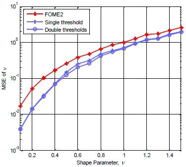
In order to assess performances of the proposed approaches for the case of high CNR (CNR=5dB) and M = 1000, Figure 7 indicates the best MSE results of single and double thresholds methods. For 0.4<v<1, the performance of double thresholds method is considerably improved compared with the single threshold estimator. Computation time of the proposed thresholding estimators are much lower than the numerical [zlog(z)] approach. In the light of the above analysis, the Otsu’s based estimation methods achieve globally better estimation performances than other methods.
Table 1. Bias of v estimates (i.e. $|E(v-\hat{v})|$) using existing and proposed estimators for M=1000 and N=1
|
v |
CNR |
HOME |
[zlog(z)] |
MFOM1 (p=0.5) |
MFOM2 (p=-0.5) |
Single threshold |
Double thresholds |
|
0.1 |
0dB |
0.2585 |
0.0526 |
0.0472 |
0.4139 |
0.0472 |
0.0472 |
|
0.5 |
9.1867e+4 |
0.3646 |
4.3832 |
1.8326 |
0.4416 |
0.4817 |
|
|
1 |
3.0247e+4 |
3.3633 |
31.5963 |
3.7986 |
1.4354 |
1.5421 |
|
|
1.5 |
1.0769 e+4 |
7.0443 |
1.834 e+3 |
6.1709 |
2.1721 |
2.3116 |
|
|
0.1 |
5dB |
0.2093 |
0.0323 |
0.0334 |
0.1121 |
0.0334 |
0.0334 |
|
0.5 |
1.6866 |
0.1406 |
0.1650 |
0.5608 |
0.1586 |
0.1564 |
|
|
1 |
899.6082 |
0.5288 |
65.0361 |
0.8864 |
0.3518 |
0.3881 |
|
|
1.5 |
3.3757e+3 |
1.8903 |
3.1740 e+3 |
1.4004 |
0.6414 |
0.7226 |
|
|
0.1 |
10dB |
0.2021 |
0.0238 |
0.0248 |
0.0433 |
0.0248 |
0.0248 |
|
0.5 |
0.8840 |
0.0703 |
0.1148 |
0.1575 |
0.1148 |
0.1132 |
|
|
1 |
23.2784 |
0.2478 |
0.4487 |
0.3104 |
0.2603 |
0.2590 |
|
|
1.5 |
9.6863 |
0.6496 |
22.0353 |
0.4689 |
0.2230 |
0.2730 |
Figure 3. MSE of v estimates of K-clutter plus thermal noise distribution for CNR = 0dB and M = 1000
Figure 4. MSE of v estimates of K-clutter plus thermal noise distribution for CNR=0dB and M=700
Figure 5. MSE of v estimates v of K-clutter plus thermal noise distribution for CNR = 0dB and M = 2000
Figure 6. MSE of v estimates of K-clutter plus thermal noise distribution for CNR=-5dB and M=1000
Table 2. Variance of v estimates (i.e. $E\left[(\hat{v}-E[\hat{v}])^{2}\right]$) using existing and proposed estimators for M=1000 and N=1
|
v |
CNR |
HOME |
[zlog(z)] |
MFOM1 (p=0.5) |
MFOM2 (p=-0.5) |
Single threshold |
Double thresholds |
|
0.1 |
0dB |
0.0780 |
0.0062 |
0.0064 |
0.0381 |
0.0064 |
0.0064 |
|
0.5 |
8.4095e+12 |
0.7475 |
8.3362 e+3 |
0.6290 |
0.8791 |
0.9811 |
|
|
1 |
9.3059 e+11 |
206.9979 |
4.5382 e+4 |
4.4025 |
7.3816 |
7.2389 |
|
|
1.5 |
3.6165 e+10 |
187.8564 |
1.4954 e+9 |
19.8325 |
17.5637 |
16.5407 |
|
|
0.1 |
5dB |
0.0382 |
0.0024 |
0.0028 |
0.0045 |
0.0028 |
0.0028 |
|
0.5 |
68.2367 |
0.0977 |
0.1500 |
0.0558 |
0.1136 |
0.1085 |
|
|
1 |
3.3240e+8 |
2.0333 |
4.0599 e+6 |
0.2215 |
0.5670 |
0.6262 |
|
|
1.5 |
5.5027e+9 |
169.2435 |
9.9909 e+9 |
0.6625 |
1.7136 |
1.6844 |
|
|
0.1 |
10dB |
0.0379 |
0.0017 |
0.0019 |
0.0018 |
0.0018 |
0.0019 |
|
0.5 |
3.1032 |
0.0438 |
0.0625 |
0.0227 |
0.0625 |
0.0596 |
|
|
1 |
5.6250e+4 |
0.3315 |
1.1050 |
0.0908 |
0.2902 |
0.2982 |
|
|
1.5 |
1.9491e+8 |
2.4487 |
2.0157 e+5 |
0.2299 |
0.2299 |
0.5866 |
Figure 7. MSE of v estimates of K-clutter plus thermal noise distribution for CNR=5dB and M=1000
To overcome estimation issues for the case of a single look data of K-clutter plus noise parameters using either [zlog(z)] or MFOME method, new estimation procedures based on switching techniques were proposed in this work. Single threshold and double thresholds were considered and Otsu’s algorithm was carried out off-line to select appropriate values of underling thresholds. Simulation experiments were worked out and showed that the single threshold and double thresholds based methods start by tracking the FOME1 for low values of the shape parameter and then tracks the FOME2 for high values of the shape parameter. Compared with existing moments methods and numerical [zlog(z)] method, lower MSEs of the estimates were achieved by the proposed estimators with a small computation time. The extension of this work should use adaptive thresholds in order to get better estimates particularly in cases of low CNR.
[1] Posner, F.L. (2002). Spiky sea clutter at high range resolution and very low grazing angles. IEEE Transactions on Aerospace and Electronic Systems, 38(1): 58-73. http://dx.doi.org/10.1109/7.993229
[2] Rosenberg, L., Watts, S., Bocquet, S. (2014). Application of the K+Rayleigh distribution to high grazing angle sea-clutter. 2014 International Radar Conference, Lille, France. http://dx.doi.org/10.1109/RADAR.2014.7060344
[3] Anastassopoulos, V., Lampropoulos, G.A., Drosopoulos, A., Rey, M. (1999). High resolution radar clutter statistics. IEEE Transactions on Aerospace and Electronic Systems, 35(1): 43-60. http://dx.doi.org/10.1109/7.745679
[4] Watts, S. (1987). Radar detection prediction in K-distributed sea clutter and thermal noise. IEEE Transactions on Aerospace and Electronic Systems, 23(1): 40-45. http://dx.doi.org/10.1109/TAES.1987.313334
[5] Mezache, A., Sahed, M., Laroussi, T., Chikouche, D. (2011). Two novel methods for estimating the compound K-clutter parameters in presence of thermal noise. IET Radar Sonar and Navigation, 5(9): 934-942. http://dx.doi.org/10.1049/iet-rsn.2010.0296
[6] Bocquet, S. (2015). Parameter estimation for pareto and K distributed clutter with noise. IET Radar Sonar and Navigation, 9(1): 104-113. http://dx.doi.org/10.1049/iet-rsn.2014.0148
[7] Mezache, A., Sahed, M., Soltani, F., Chalabi, I. (2015). Estimation of the K-distributed clutter plus thermal noise parameters using higher order and fractional moments. IEEE Transactions on Aerospace and Electronic Systems, 51(1): 733-738. http://dx.doi.org/10.1109/TAES.2014.130572
[8] Sahed, M., Mezache, A., and Laroussi, T. (2015). A novel [z log(z)]-based closed form approach to parameter estimation of k-distributed clutter plus noise for radar detection. IEEE Transactions on Aerospace and Electronic Systems, 51(1): 492-505. http://dx.doi.org/10.1109/TAES.2014.140180
[9] Sahed, M., Mezache, A. (2017). Closed-form fractional-moment-based estimators for k-distributed clutter-plus-noise parameters. IEEE Transactions on Aerospace and Electronic Systems, 53(4): 2094-2100. http://dx.doi.org/10.1109/TAES.2017.2667588
[10] Bocquet, S., Rosenberg, L., Gierull, C.H. (2020). Parameter estimation for a compound radar clutter model with trimodal discrete texture. IEEE Transaction on Geoscience and Remote Sensing, 1-12. http://dx.doi.org/10.1109/TGRS.2020.2979449
[11] Otsu, N. (1979). A threshold selection method from gray-level histograms. IEEE Transactions on Systems, Man, and Cybernetics, 9(1): 62-66. http://dx.doi.org/10.1109/TSMC.1979.4310076
[12] Yu, F.J., Sun, W.Z., Li, J.J., Zhao, Y., Zhang, Y.M., Chen, G. (2017). An improved Otsu method for oil spill detection from SAR images. Oceanologia, 59(3): 311-317. https://doi.org/10.1016/j.oceano.2017.03.005
[13] Messina, M., Greco, M., Fabbrini, L., Pinelli, G. (2012). Modified Otsu's algorithm: A new computationally efficient ship detection algorithm for SAR images. Tyrrhenian Workshop on Advances in Radar and Remote Sensing (TyWRRS), Naples, 262-266. http://dx.doi.org/10.1109/TyWRRS.2012.6381140
[14] Zeggada, A., Melgani, F., Bazi, Y. (2017). A deep learning approach to UAV image multilabeling. IEEE Geoscience and Remote Sensing Letters, 14(5): 694-698. http://dx.doi.org/10.1109/LGRS.2017.2671922