Sravani Nannapaneni | Venkatramaphanikumar Sistla* | Venkata Krishna Kishore Kolli
© 2020 IIETA. This article is published by IIETA and is licensed under the CC BY 4.0 license (http://creativecommons.org/licenses/by/4.0/).
OPEN ACCESS
Generative Adversarial Networks (GAN) generates model approaches using Convolution Neural Networks (CNN) to find out learning regularities and to discover the hidden patterns held in given input data. GAN is a generative model that is trained using two models such as generator and Discriminator both competing against each other to learn the probability distribution function, networks such as CNN, RNN, ANN etc. These traditional neural networks are easily fooled in misclassifying things by adding small amount of noise to original data, whereas GAN’s are more stable and easier to train due to the amalgamation of Feed Forward Neural Network and CNN. In general, GAN’s are simple Neural networks be trained in adversarial way to generate the data mimicking same distribution, Generator learns new possible sample, and the Discriminator learns how to differentiate generated samples from valid facts. Generated samples are similar in the nature but different from real distribution data. The generated samples make use of computer vision techniques such as visualization designs, realistic image generation, image classifications etc. In the proposed work, to realize the probability distribution Restricted - Boltzmann machines and Deep Belief networks are used. The performance of the GAN Networks is evaluated on various standard datasets to realize the complex tasks such as image prediction, handwritten digit’s generation, clothing classification, image segmentation tasks etc. From the experimental results, it is clearly evident that the performance of GAN outperforms other state of the art classifiers on all the benchmark datasets.
distributed system, task scheduling, load balancing, fuzzy c-means, hungarian method
Deep generative models come under the powerful class of unsupervised machine learning these models are applied for different types of applications such as image to image conversion, photograph editing, high-resolution images, classification, image generation, learned compressions, domain adaption. GAN’S are introduced in the year 2014 by Ian Good Fellow and other researchers at the University of Montreal including Yoshua Bengio GAN’S are cleverly training the generative models by framing the problem as supervised learning problem with two models that is Generator (e.g. generate duplicate copies of photos that looks like a real photos) And Discriminator (e.g. it will differentiate the generated photos and real photo), actually the Discriminator will act as classifier it will classify the whether it is an original or fake [1]. Basically, GAN’s have the ability to predict features in a more adversarial manner; with that both generator and discriminator are competed with each other during the training. Once they are well trained, they have the ability to create an image and piece arts etc. During this training of discriminator, generator is kept as constant, like wise during the training of generator; discriminator will be kept as constant. GAN’S are cleverly training the generative models by framing the problem as supervised learning problem with two models that is Generator and Discriminator [2]. In this two models are train together until we get the situation like zero-sum (or) min-max game, at certain time period the generator unable to generate a data and the discriminator unable to classify the data sample i.e. is which one is real and which is fake this situation called as a Nash-Equilibrium. In this situation whether two players can improve the learning independently [3]. In the same way generator and discriminator networks usually parameterized in deep neural networks hard to decide min-max problem. In implementation training performed use stochastic gradient descent (SGD) it will learning process held few samples were chosen randomly instead of the whole dataset, adaptive learning rate optimization (ADAM) is used to find the individual learning rate for each parameter, GAN training is sensitive to the choice of loss functions optimization of each player in NN architectures so that purpose applies the Regularization and Normalization techniques [4, 5].
Figure 1. Architecture of GAN
The main objective of the generator is will generate an image that will look like an original image similarly the goal of the discriminator is classify weather it is an actual image or forged image. The generic architecture of GAN is given in Figure 1.
Related work is presented in Section II, basic functionalities of Tensor Flow are given in Section III, Experimental results and discussions are given in Section IV and finally Conclusion is presented in Section V.
GAN is a word comprises of three different parts i.e. generative, adversarial; networks to study the generative model which describes facts generated probabilistic distribution. And adversarial means training is done by adversarial settings and networks for deep neural networks and AI algorithms for training purpose Generator will generate forged samples from the given information it may be either audio or video or images, here the generator tries to make a discriminator is a fool, other hand discriminator can distinguish which one is real and which one is fake both NN can competing with each other during a training phase. This phase, several steps are repeated both networks get their better and better performance in each repetition [6].
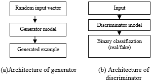
Generator and discriminator architecture GAN, models do not directly use pair of input and output, instead of that learns how inputs and outputs can be paired it is used for testing the ability to use high-dimensional complicated probability distribution (Figure 2). It will simulate features for planning, Generator uses up-sampling it learns joint probability distribution. A Generator will work for classification and regression. While discriminator learns the boundary between the classes it learns conditional probability distribution, discriminator uses down-sampling it is a binary classifier.
Figure 2. Basic architectures of generator and discriminator
2.1 Concepts related to GAN
KULLBACK - libeler divergence (KL divergence) is known as relative entropy This method is used to find similarities between the two probability distribution .it will measure the how one probability distribution p diverges from a second expected probability distribution q,KL divergence will be minimum or zero [4], KL divergence equation to calculate the probability distributions is as the following Eq. (1).
$\mathrm{D}_{\mathrm{KL}}(\mathrm{p} \| \mathrm{q})=\int x^{\mathrm{p}(\mathrm{x}) \log \frac{p(x)}{q(x)}} d x$ (1)
From the above equation, DKL represents the KULLBACK - Libeler divergence, in this divergence, has asymmetric nature, here p(x), q(x) is two probability distributions. The distance between the p(x) is similar to q(x) but the distance between the q(x) top(x) is not same. Here distance should not be used as a metric.
2.2 Jensen – Shannon divergence
It is also called information radius (or) total divergence to the average. It is another method to calculate the similarities between the two probabilities. In Jensen-Shannon divergence has symmetric nature, due to this nature we have a possibility to measure the distance as a metric, and we take the square root JS-divergence we get JS- distance.
$\mathrm{D}_{\mathrm{JS}}^{(\mathrm{p} \| \mathrm{q})}=\frac{1}{2} \mathrm{D}_{\mathrm{KL}}\left(\mathrm{P} \| \frac{p+q}{2}\right)+\frac{1}{2} \mathrm{D}_{\mathrm{KL}}\left(\mathrm{q} \| \frac{p+q}{2}\right)$ (2)
The above equation is used to calculate the probability distribution, DJSis Jensen – Shannon divergence DKL is KULLBACK – libeler divergence and (p+q) is mid-point measure.
2.3 Mathematical modelling in GAN
To train GAN’s we have two different networks i.e. generator and discriminator, while training process we must keep generator constant during the discriminator training phase. Discriminator training tries to distinguish original or fake, it has to learn to recognize the flaws of the generator. Similarly, we keep the discriminator constant during the generator training process. In this, both neural networks during training processes can compete with each other the training process will be repeated several times until both networks get better and better with their individual jobs [7]. Generator model will capture the distribution of data and it is trained and tries to maximize the probability of discriminator making mistakes. In other hands, discriminator will estimate the probability of sample it acknowledged from training data not from the generator. Both KL-divergence and Jensen-Shannon divergence used for the training model.
The trained generative model tries to maximize the probability of discriminator make mistake. Probability estimation of sample based on the model not from the generator produced data. Discriminator tries to minimize its rewards. The Mathematical formula for min-max is as follows:
$\operatorname{Min}_{\mathrm{G}} \operatorname{Max}_{\mathrm{D}} \mathrm{V}(\mathrm{D}, \mathrm{G})=\mathrm{E}_{\mathrm{X} \sim \mathrm{P} \operatorname{data}(\mathrm{x})}[\log \mathrm{D}(\mathrm{x})]^{+} \mathrm{E}_{\mathrm{Z}}$
$\sim \mathrm{p}_{\mathrm{z}(\mathrm{z})}[\log (1-\mathrm{D}(\mathrm{G}(\mathrm{Z})))]$ (3)
$\begin{aligned} \operatorname{Max}_{\mathrm{D}} \mathrm{V}(\mathrm{D}) &=\mathrm{E}_{\mathrm{X} \sim \mathrm{P} \operatorname{data}(\mathrm{x})}[\log \mathrm{D}(\mathrm{x})]^{+} \mathrm{E}_{\mathrm{Z} \sim \mathrm{p}_{\mathrm{Z}(\mathrm{z})}} \\ &[\log (1-\mathrm{D}(\mathrm{G}(\mathrm{Z})))] \end{aligned}$ (4)
Optimization at the generator to fool the discriminator
$\operatorname{Min}_{\mathrm{G}} \mathrm{V}(\mathrm{G})=\mathrm{E}_{\mathrm{Z} \sim \mathrm{p}_{z}(\mathrm{z})}[\log (1-\mathrm{D}(\mathrm{G}(\mathrm{z})))]$ (5)
$\mathrm{p}(\mathrm{x}, \mathrm{y})=\mathrm{p}(\mathrm{x} | \mathrm{y}) \cdot \mathrm{p}(\mathrm{y})$ (6)
From the above equation x, y are random variables, similarly, for discriminator, conditional probability distribution
$\mathrm{p}(\mathrm{y} | \mathrm{x})(\text { i.e. probability of } \mathrm{y} \text { given } \mathrm{x}$ should be maximum) (7)
2.4 GAN loss functions
The Architecture involves the simultaneous training of two models i.e. generator and discriminator. During the training of generator we drop the other one, it reflects the distribution of actual data. Both generator and discriminator loss functions look will unlike at the ending. The Loss function described by Ian Good fellow et al. can be derived from the formula of binary cross-entropy. Loss at discriminator real data is define as Dlossreal = log (D(x)) And for fake data is define as Dlossfake = log (1-D (G (Z))) and to find the total loss at discriminator is Dloss = Dlossreal + Dlossfake [8]. Similarly the loss function at creator is defined Gloss = log (1- D(G(z))) (or) -log (D(G(z))). Formulas for finding the total cost at discriminator and generator are as following equations.
Total cost at discriminator is $\frac{1}{m} \sum_{i=1}^{m} \log \left(D\left(x^{\mathrm{i}}\right)+\log \left(1-\mathrm{D}\left(\mathrm{G}\left(\mathrm{Z}^{\mathrm{i}}\right)\right)\right)\right.$ (8)
Total cost at generator is $\frac{1}{m} \sum_{i=1}^{m} \log \left(1-D\left(G\left(Z^{\mathrm{i}}\right)\right)\right)$ (9)
As we can see above equations discriminator network runs twice one is real data, another is for fake data before it can calculate the final loss function generator runs only once, once we got the two-loss functions we have to calculate the gradients concerning to their parameters, Back-propagation can be done through their networks independently [9].
2.5 GAN objective functions
The Discriminator is a binary classifier to feed real data. The Model must generate a high probability for actual data and low probability for false data. The main objective of GAN functions is to learn some hidden facts about data in the classification of real and fake images by extracting the features manually and automatically in an efficient manner with low cost.
Variables and functions of GAN’s are specified below [10]. Z- is the input noise data, G(Z)-fake generator output-real data training sample, D(X)- discriminator output for actual data whose values are in between 0-1, D(G(z))- discriminator output for invalid data.
The Discriminator is a binary classifier to feed real data. The Model must generate a high probability for actual data and low probability for false data (generator produced output), the main objective is to learn some hidden facts of data. Variables and functions of GAN’s are specified below [10]. Z- is the input noise data, G(Z)-fake generator output-real data training sample, D(X)- discriminator output for actual data whose values are in between 0-1, D(G(z))- discriminator output for invalid data.
From the above D(X), D (G (Z)) gives a score between 0 and 1. At discriminator D(X) should maximized the real data while minimizing the fake data i.e. D(G(Z)), G (z) produces a same shape of data but it has some noisy data, we want to build a model for generator that maximizes the fake data i.e. D(G(Z)), Actually generator use pair of inputs and outputs to tell the model to do, whereas discriminator learns how the input and outputs can be paired, the main strategy of discriminator is estimating the ratio using supervised learning is the key approximation mechanism used by GAN’s.
2.6 Challenges with GAN
Mode collapse which means the generator will be stuck at one point producing a limited number of samples during training or after training, generator keep on producing the same image several times repeatedly this leads to complete model collapse. Whereas the generator learns very few properties and produces few varieties of samples is called partial model collapse. Another problem with GAN’s is vanishing gradients. This problem will persist if there is no stability in training of GAN’S. Unsupervised learning is a more challenging task when compared to supervised learning because it doesn’t have a label.
The Third problem is hard to find NASHEQUALIBRIUM because in both networks Competent with each other I.e. non-cooperative game. The fourth problem is counting, and testing features, we can’t differentiate the images that have two eyes or multiple eyes. The Fifth problem is the problem with a perspective which means GAN’S fail to differentiate front and back view, 2-D representation converted into 3-D objects, another problem with GAN’s are global structures it means can’t recognize the bottom and top positions for example cow in hind legs position and folding leg positions. GAN requires images with high dimensional data because it has many variations in case of view point, illumination etc. to overcome this limitation finding the hidden and latent vectors.
To overcome the above problems, we have different types of GAN’S i.e., vanilla GAN’s in this type of GAN’S are simple here both networks are simple with multi-layer perceptron’s. And algorithms simple and to optimize the mathematical equations used in SGD, whereas in case of conditional GAN’s used some conditional parameters; here some additional parameters are added to the generator to generate a corresponding data. Whereas deep convolution GAN’s (DCGAN) use the convolution network layers instead of multi-layer perceptions. In DCGAN layers are not fully connected [11]. Another type is super-resolution i.e. SRGAN’S here DNN along with adversarial networks in-order to get the high-resolution images.
Tensor flow is an open-source platform to integrate as well as develop large scale AI and deep learning models. Tensor flow is a machine learning framework originally developed by Google [12]. One of the advantages is it can be easily modified, share and integrate, training, designing, building because all the blueprint features are open to all. And also expand particular software and the product it can support various web, mobile, and programming languages and IoT applications [13]. Tensor flow library is used for numerical computations, using data flow graphs. Nodes signify the operations, edges signify the facts, it supports programming languages such as C++, GO, Julia, swift and RUST, C#. along these it can support hardware acceleration for running large scale machine learning codes it includes CUDA (library for running machine language code on GPU’s, TPU’s is a custom hardware processing unit it especially designed and developed to process tensors automatically computing their derivatives, tensors can be viewed as a multi-dimensional array of numbers. This will be used at the backend. Tensor Flow supports computations across multiple CPUs and GPUs. This means to improve the speed of the training computations can be allocated across the devices and its architecture is given in Figure 3. By performing parallelization, there is no need to wait for weeks to get the results of algorithms. Tensor Flow provides two versions, and they are Tensor Flow with CPU version supports device doesn’t run on NVIDIA GPU, simply you can install TensorFlow with GPU version, it supports for earlier computation. This version needs only strong computational capacity, similarly, TPU supported for the cloud [14].
Figure 3. Overview of tensor flow architecture
Data sets contain a collection of facts example it contains features significant to solve the problem. Features Important pieces of data that help us understand a problem. These are feed into a Machine Learning algorithm help to discover, we have different types of datasets like MNIST it contains images for handwritten digit classification and CIFAR-10 which contains images it can be broken into ten different classes. Datasets can be categorized into training and test set. The training set teaches different features by adjusting the parameters according to the likelihood of minimizing the errors. Whereas the test set can’t use until the end. After the trained and optimized the data, test the neural network against the random sampling, It can validating the results accurately in case we don’t get the accurate results then go back to look at the hyper parameters in training set .to achieve the quality of data tune the network and look at preprocessing technique.
4.1 MINST classification clothing images
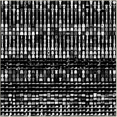
To train the neural networks model to classify the MNIST simple fashion dataset it contains 70,000 gray-scale images with 10 different categories, cloth images like it is a shirt, trouser, pullover, dress, sneaker, shoes, handbags, pants, coats accurately 10, 000 images are used. system learn to classify the images and pixel values are ranging from 0-255, and label values are representing as integer values those ranges represented as 0-9, each image is mapped with a single label. Sample MINST fashion dataset is shown in Figure 4.
Figure 4. MINST fashion dataset
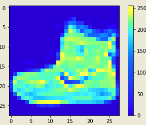
To preprocess the data for the training network to see the pixel values whose range is from 0-255. And scale those values are ranging from 0-1 to train neural network model, like that we have to train and test the data same process, Next step we have to build the model for that we take the layers i.e. flatten, 2 dense layers, first layer is flattened layer transform the images into 2-dimensional array of pixels size is (28x28) to one-dimensional array (28x28) it has no parameter to discover so reformat the information. After that pixel is arranged into vector format, the network model consists of sequence layers which are either fully or densely connected neural network layers. The first and second dense layer has (128, 10) nodes with activation function SOFTMAX it will return probability score amount is one. The probability of a present image belongs to 10 classes it indicates each node. The Next step is compiling the model for this measure the loss function, optimizer, and metrics. Sample image before preprocessing and 25 images before training are given in Figure 5.
(a) Sample image before preprocessing
(b) First 25 images of training set and scale the image values to feed NN whose Range 0-1
Figure 5. Images before training
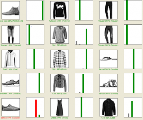
Figure 6. Correct and incorrect predicted image
To measures the accuracy of the model during the training use the loss functions, optimizer defines the update the model based on the data, metrics are used to monitor the training and test data that are to be correctly classified. After compile the model we have to train the model it contains the steps, feed to train the model after that model learns the associate images and labels, and model can predict the test data for these use model. fit, after 10 epochs get the 91% accuracy, Next step is to evaluate the accuracy-test data compare how model performs, it returns the accuracy is 88% for test data. The result will be slightly less when to compare the training set accuracy .so the difference between the training and test accuracy leads to model over- fitting because of hat model performs worse to train new input data. After that we have to make the prediction about the images, for this prediction label for each image in testing data prediction of a group of ten numbers represent the model confidence images of ten different articles of clothing, the Correct prediction label represents green and incorrect label represents red color for the predicted label. Performance evaluation on sample image is given on Figure 6.
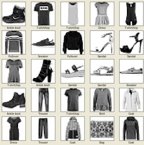
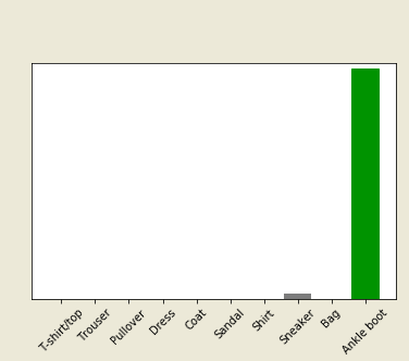
Finally, the model is trained to make the prediction about the single image. To optimize the model, make the prediction on batch or group of examples at one time and presented in Figure 7.
(a) Test images with predicted labels
(b) Predicting A particular image over a batch of images
Figure 7. Test and predicted image outcome
4.2 Performance evaluation on MNIST dataset
MNIST means the modified national institute of standards and technology. The main aim is identified digits from a dataset tens and thousands handwritten pictures for this approach we use KERAS in tensor flow as backend and for prediction purpose use the neural networks that must be 4layer or 5layers experimenting with various optimizers SGD, ADAM. First step import the libraries and read the data which contain the (5X785) it means 1 label and 784 features.
The Next step to divide the data into the training and validation data set (28000, 784). Then perform the data cleaning and normalization operations so we get the pixel value range between the 0-255 so we have to normalize the features so we have to convert our labels from a class vector to binary ONE HOT ENCODED. After that perform model fitting by using neural networks models and collect the accuracy model which perform the best validation it will be used for competition (Table 1).
Model 1: Simple neural networks with 4 – layers (300, 100, 100, 200) and using the activation function is RELU and to determine the output use SOFTMAX function. Model has six input layers, four hidden layers and one output layer with 2, 97,910 parameters to estimate. Then insert the hyper parameters with learning rate 0.1, the number of training epochs is 20, batch size 20, to compiling the model use the categorical cross-entropy is used as a loss function and accuracy can be measured as metrics, SGD is used as an optimizer. We achieved a training score of around 96-98% and a test score of around 95-97%.
Model 2: In this model change the optimizer as ADAM by maintaining the same parameters values it tends to perform the better performance tends to an average of 1.5-2.5% so go forward ADAM as an optimizer choice by changing different learning rate 0.1 – 0.01 and 0.5 and test the accuracy.
Model 3: In this model learning rate is 0.01, and number of training epochs20, with the batch size is 20, categorical cross-entropy used as loss function and accuracy is measured as metrics, ADAM has used an optimizer we get the accuracy is 97%.
Model 4: In this model use the learning rate 0.5, with number of training epochs is 20, with batch size is 20, use categorical cross-entropy as loss function and accuracy is measured in metrics, ADAM is used as an optimizer we will get the accuracy around 98%. As per three different learning rates 0.01, 0.1 and 0.5 we get 98%, 97%, 98% respectively there is no change in changing the learning rate so take default learning rate 0.01. So we have to proceed to fit NN with 5 – hidden layers with set of (300, 100, 100, 100, 200) we will set the training epochs is 20 and training batch size=100. When compared to the first model adding an additional layer didn’t get any improvement in accuracy this leads to more computational cost by adding additional layer to our neural network, so we will stick on 4- layer neural network. To prevent the over-fitting we will include the dropout rate is 0.3. The model has six input layers, four hidden layers, one output layer estimating parameters 2,97,910 validation score is close to 98% so we proceed to use this model to predict the test set.
Table 1. Performance evaluation using GAN with ADAM optimizer
|
Layers |
Learning rate |
Epochs |
Batch size |
Training Accuracy |
Validation accuracy |
|
4 |
0.01 |
20 |
100 |
98% |
96% |
|
4 |
0.5 |
20 |
100 |
98% |
97% |
|
5 |
0.01 |
20 |
100 |
98% |
96% |
The Dataset contains both cats and dogs we have to classify the images. To build a model using the sequential model, import the required packages then load the dataset dogs Vs cats after that the data set can be split into train and validation sets both contain dogs and cats. Sample Dogs & Cats after applying various arguments are presented in Figure 8.
After extracting the contents assign the paths for both the train and validation dataset, to understand the data look at how many numbers of dogs and cats present in the training and validation data set. Total training cat and dog images are (1000, 1000) and entire validation cat and dog images (500,500) so whole training images are 2000 and validation images are 1000.To preprocess the data set to the training network set up the variables for our convenience with batch size=128, epochs=15, image height and width is =150. After that to prepare the data, arrange the images into floating-point tensors arrange them properly for network training, decode the images and change into an appropriate grid format as RGB format. Rescale the values of the tensor range 0-255 to 0 -1. NN choose little input values, defining generators training and validation images apply to rescale and resize the images into required dimensions found 2000 images belong training generator and found 1000 images belongs to validation generator.
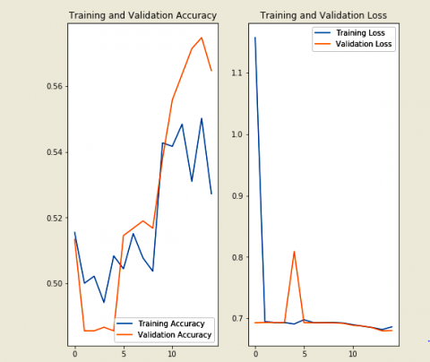
To create model batch images from training generator are extracted for visualization, the model consists of three convolution layers with MAXPOOL each of them are connected with a fully connected layer with units 512. on the top with the activation function is RELU outputs are binary classification activation function is SIGMOID, Compile the model ,To train the model use fit_ generator and image_ generator methods after the 15 epochs we get the training accuracy is 95% and validation accuracy is 73% there will be lot of difference by increase the performance of both training and validation dataset, this leads to a method over-fitting due to this reason generalization is difficult so we need to pass DATA ARGUMENTATION, Data argumentation approach generates additional training data from the existing samples by using random transformations the Main goal is the exact sample picture will never see during the training process.
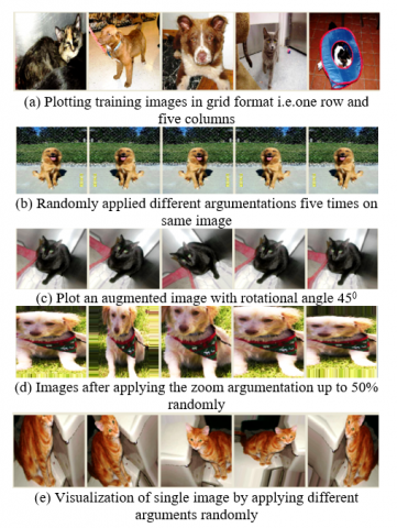
Next step to pass the arguments like horizontal flip to see the same image repeat it five times, then took different argumentations, ROTATION randomly at 45 degrees for training images, apply another argumentation by zooming up to 50% randomly, After that put it into all together that is shift width and height, rotation and scaling, zoom operations all these arguments see in a single image. Similarly, apply this validation generator. Another method is used to reduce the over-fitting i.e. dropout here distribute the weights to the network apply the dropout to the layers initially set to be zero, the outputs are applied during training process dropouts takes a fractional value like 0.1, 0.2. Randomly apply the output layers, drop out applying layer it kills the 10% of units for each training epochs. Finally apply the dropout of first and last MAXPOOL layers set 20% for training epoch then compile the model will get the accuracy is 61% and validation accuracy is 66% so we can see less over-fitting when compared to the previous method after training more number of epochs. Performance evaluation such as accuracy and loss functions of proposed method on Dogs vs Cats dataset during training and validation phases is presented in Figure 9 and Figure 10.
Figure 8. Variations in dogs and cats images after applying different arguments
Figure 9. Visualization graph for training validation accuracy and loss
Figure 10. Visualizing the new model after training significantly less over fitting than before
4.4 CIFAR-10 image dataset
CIFAR-10 dataset is a recognized computer visualization used for the identification of objects. it contains 60,000 color images with ten different classes, like horse, bird, automobiles, cat, frog, deer, truck. Each class contains 6,000 images. The dataset is split into training and testing images are (50,000 and 10000) there is no overlap between the classes because they are mutually exclusive, after that normalize the pixel values whose range values are between 0-1. Sample CIFAR-10 dataset is shown in Figure 11.
Figure 11. First 5 images with their class labels
The Next step is to verify the data the dataset looks accurate, so plot the first five images along with display the class name below each and every image from training data set, after that create a convolution base using a regular model use conv2D, max-pooling 2D layers. CNN takes tensors to shape like image height, width, and color _ channels as an input ignore batch size, color channels refer to RGB in this process configure the input shapes (32, 32, 3) it is the format of CIFAR image we can pass the arguments for input _ shape for the first layer.
Figure 12. Model evaluation graph for test and validation accuracy
In this dataset use the sequential model total number of parameters 56,320 and trainable parameters are 56,320 then to complete the model add the dense layers on top, feed the model tensor last output from the convolution base with shape (3, 3, 64) to do classification, Dense layers take 1D vectors as input while the 3D tensor its present output. First, flatten the 3D output into 1D then add another one denser layer on the top, CIFAR has ten output classes so use the 10 outputs for final dense layers, and SOFTMAX is activation function, a sequential model used for a model summary, in this the total number of trainable parameters is 1, 22,570. To train and compile the model use the ADAM optimizer, sparse categorical cross-entropy used for the loss function, accuracy is measured in metrics, epochs = 10, we get the accuracy is 77% and validation accuracy is 70%, Evaluate the model we get the test accuracy is 70% (Figure 12).
4.5 Image segmentation oxford-IIIT data set
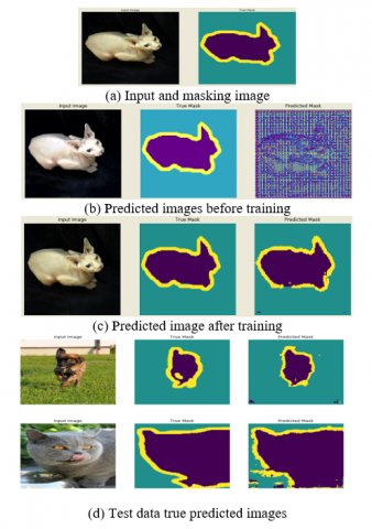
Image segmentation is used to know the particular object location, shape, and its pixel values, to perform the segmentation operations to image specify the label name to each pixel, to perform image segmentation train the neural network outputs of image masking pixel-wise, The oxford – IIT pet dataset consists of images and labels with pixel-wise mask each pixel can be categories three ways, pixel belongs to pet, pixels bordering the pet and surrounding pixels, First download the pets’ dataset with segmentation masks, performing the operations like flipping images then normalize the image whose range between 0-1, segmentation masks are labeled as 1, 2, 3... For our convenience subtracting 1 for segmentation masking resulting values are 0, 1, and 2. Then the dataset can be split into a test and train. Sample Images of Oxford IIIT Data set is given in Figure 13.
Figure 13. Training and test set outcomes
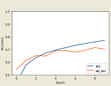
The Next step is to define the model here apply the down-sampling for encoding and up-sampling for decoding, to learn the features reduce the number of trainable parameters for encoding pre trainable model is used. Encoder task will be pre-trained by mobileNetv2 model intermediate outputs will be used decoder un-sample block it is already implemented by tensor flow examples. It contains a 3 output channels because there are three possible labels for each pixel here perform the multiclass classification where each pixel classified into 3 classes Encoder consists of specific output for intermediate layers in model here encoder will not be trained during the training process. Decoder un-sample blocks are implemented by tensor flow examples. Next step is to train the model optimizer = ADAM, sparse_ categorical_ cross-entropy is used as a loss function, metrics= accuracy use the loss function because the network is trying to assign each pixel label just like a multi-class prediction true segmentation mask for each pixel has either 0, 1, 2. The Network has a three output channels each and every channel is to predict the class and loss function to predict the mask function assign the label to the pixel to the channel with the highest value, To make the predictions after 20 epochs we get the training accuracy is 93% and validation accuracy is 87%. Training and validation loss after 20 epochs are given in Figure 14.
Figure 14. Training and validation loss graph after 20 epochs
4.6 Hand written digits generation
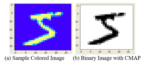
In any neural networks, we have inputs and output nodes and having some hidden layers each input layer is connected with the hidden layers with weights, connected with one hidden layer is a network and connected with 2 or more hidden layer is a deep neural network, activation function specifies whether the neuron is a fire or not fire. Import the required packages and download the MNIST dataset with the size 28x28 resolution contain the images are hand-written digits 0-9, then it will be divide into train and test dataset, then print all the train data it displays all the tensor values after that we have to show the images by importing the MATPLOTLIB it displays colored image if you want gray scale images use camp, after doing this we have to normalize the data for both train and test data whose axis value is one. It will be representing the result tensor values are between 0-1. Next step we have to build the model for this use the sequential model and the layers for that model i.e. flatten layer, and add another layer is dense layer we have to provide the parameters (128, activation function = RELU) and add another dense layer for classification use (10, activation function = SOFTMAX) this will define the architecture of model. Next step we have to train the model and compile the model is optimizer= ADAM, loss = sparse _ categorical _ cross-entropy, and metrics = accuracy, to train a model epochs=5 accuracy achieved after training model is about 98%, Next thing is to evaluate the model value accuracy we get 97% there will be a slight difference between the training models and evaluate model there will be less over-fitting after that save the model in epic _ num _reader model then find the prediction for test data we get the result differently those are probability distributions. For this import NumPy and pass the parameters as ARGMAX for predictions with index value, it will show the image of sample color and binary given in Figure 15.
Figure 15. Sample colored and binary image
Avoid the mode collapse using the VEEGAN’S, SGD (distribution min and max), another method is mini-batch discrimination here compute independently each point by dividing into small batches. Another problem is the vanishing gradient to reduce this problem activation function transform values are in the range of 0, 1 and use the optimizers to reduce the loss functions and use the chain-rule for back propagation. The third problem is Nash-Equilibrium it means games can’t solve by the method of iterated elimination of dominated strategies to overcome this problem using different game strategies like a zero-sum game, constant sum, put the equilibrium point for Nash- analysis, min-max, and max-min. For lower dimensionality feature representation uses the auto-encoders unlabeled training data for encoders uses RELU, CNN. For feature, representations use dimensionality reduction, similarly for estimating the true parameters use variation auto-encoders.
Unsupervised learning is next frontier in artificial intelligence. GAN’s are established using two-layer game theory. The main aim of GAN is to predicting the correct results, to improve the performance during training process, in any situation we can train a model in worst-case scenarios also by using adversarial training. To improve performance of GAN in training, feature matching, minibatch discrimination, one-sided label smoothing, and virtual batch normalization were added. For better optimization cost function is changed and over-fitting is avoided independently at each point by splitting the data into small batches; further addition of the labels and feature matching techniques are also carried. So GAN is used to predict the performance by creating different types of models to generate the data, and capturing the data distribution and then probability distribution is computed from the training samples. Further, performance of GAN is assessed with different types of GAN’s such as vanilla, DCGAN’s, SRGAN’s to reduce the cost in the implementing of solutions for various computer vision problems.
[1] Goodfellow, I. (2016). NIPS 2016 tutorial: Generative adversarial networks. arXiv preprint arXiv:1701.00160.
[2] Goodfellow, I.J., Pouget-Abadie, J., Mirza, M., Xu, B., Warde-Farley, D., Ozair, S., Courville, A., Bengio, Y. (2014). Generative adversarial nets. In Advances in Neural Information Processing Systems, pp. 2672-2680.
[3] Mirza, M., Osindero, S. (2014). Conditional generative adversarial nets. arXiv preprint arXiv:1411.1784.
[4] Radford, A., Metz, L., Chintala, S. (2015). Unsupervised representation learning with deep convolutional generative adversarial networks. arXiv preprint arXiv:1511.06434.
[5] Kang, W.C., Fang, C., Wang, Z., McAuley, J. (2017). Visually-aware fashion recommendation and design with generative image models. In 2017 IEEE International Conference on Data Mining (ICDM), New Orleans, LA, USA, pp. 207-216. https://doi.org/10.1109/ICDM.2017.30
[6] Creswell, A., White, T., Dumoulin, V., Arulkumaran, K., Sengupta, B., Bharath, A.A. (2018). Generative adversarial networks: An overview. IEEE Signal Processing Magazine, 35(1): 53-65. https://doi.org/10.1109/MSP.2017.2765202
[7] Abadi, M., Barham, P., Chen, J.M., Chen, Z.F., Davis, A., Dean, J., Devin, M., Ghemawat, S., Irving, G., Isard, M., Kudlur, M., Levenberg, J., Monga, R., Moore, S., Murray, D.G., Steiner, B., Tucker, P., Vasudevan, V., Warden, P., Wicke, M., Yu, Y., Zheng, X.Q. (2016). TensorFlow: A system for large-scale machine learning. In 12th {USENIX} Symposium on Operating Systems Design and Implementation ({OSDI} 16), pp. 265-283.
[8] Cohen, G., Afshar, S., Tapson, J., Van Schaik, A. (2017). EMNIST: Extending MNIST to handwritten letters. In 2017 International Joint Conference on Neural Networks (IJCNN), Anchorage, AK, USA, pp. 2921-2926. https://doi.org/10.1109/IJCNN.2017.7966217
[9] Che, T., Li, Y., Jacob, A. P., Bengio, Y., Li, W. (2016). Mode regularized generative adversarial networks. arXiv preprint arXiv:1612.02136.
[10] Hua, Y., Guo, J., Zhao, H. (2015). Deep belief networks and deep learning. In Proceedings of 2015 International Conference on Intelligent Computing and Internet of Things, Harbin, China, pp. 1-4. https://doi.org/10.1109/ICAIOT.2015.7111524
[11] Kurach, K., Lucic, M., Zhai, X., Michalski, M., & Gelly, S. (2018). A large-scale study on regularization and normalization in GANs. arXiv preprint arXiv:1807.04720.
[12] Nguyen, K., Fookes, C., Sridharan, S. (2015). Improving deep convolutional neural networks with unsupervised feature learning. In 2015 IEEE International Conference on Image Processing (ICIP), Quebec City, QC, Canada, pp. 2270-2274. https://doi.org/10.1109/ICIP.2015.7351206
[13] Wang, F., Jiang, M.Q., Qian, C., Yang, S., Li, C., Zhang, H.G., Wang, X.G., Tang, X.O. (2017). Residual attention network for image classification. In Proceedings of the IEEE Conference on Computer Vision and Pattern Recognition, Honolulu, HI, USA, pp. 3156-3164. https://doi.org/10.1109/CVPR.2017.683
[14] Ertam, F., Aydın, G. (2017). Data classification with deep learning using Tensorflow. In 2017 International Conference on Computer Science and Engineering (UBMK), Antalya, Turkey, pp. 755-758. https://doi.org/10.1109/UBMK.2017.80935