Dasheng Zhang | Jing Tan* | Han Tian | Zhongzheng Wang | Wenjun Guo
OPEN ACCESS
Hydrogeological parameters are important indicators for studying aquifer properties and constructing numerical models. Affected by various unknown underground factors or human factors, there’s still a big gap between the hydrogeological parameters of aquifers calculated by different traditional pumping test methods. In recent years, artificial intelligence algorithms have been successfully applied to aquifer parameter inversion, but for a single intelligence algorithm, each has its respective shortcomings. This paper combined the quantum computing theory with the Artificial Fish Swarm Algorithm (AFSA) to improve the performance of AFSA, and then proved the correctness and superiority of the proposed method via examples.
quantum computing, artificial fish swarm algorithm (AFSA), hydrogeological parameter
For geological engineering design, groundwater numerical simulation and evaluation, beforehand, the primary task is to determine the hydrogeological parameters such as water transmissibility coefficient and water storage coefficient. Generally, the hydrogeological parameters are determined based on the data of the field pumping tests and the actual geological conditions [1]. Compared with the traditional methods such as Dupuit Equation, Thiem Equation [2], Graphical Method [3], Linear Programming [4] and Full Curve-Fitting [5], the optimized intelligence algorithms proposed in recent years have also been applied to the determine the hydrogeological parameters, for instance, there are Matlab-based Genetic Algorithm (GA), Particle Swarm Optimizatioin (PSO), etc.[6-7]. Each intelligence algorithm has its pros and cons, as well as respective applicable conditions. In the hopes of compensating for the shortcomings of single intelligence algorithm in the calculation results, this paper combined the characteristics of quantum computing and AFSA, integratedly applied the two artificial intelligence algorithms in the inversion of groundwater model parameters, and eventually analyzed the calculation results and efficiency.
From the 19th century to the early 20th century, with the development of social productivity and the advancement of science and technology, a great deal of achievements has been made in the field of physical experiments, and the quantum theory has attracted the attention of many scholars as an important theoretical accomplishment [8].
Quantum computing involves two aspects: designing new quantum algorithms, and combining quantum computing with traditional methods. At present, quantum computers have been successfully developed in China, but the application is not extensive. Therefore, combining quantum algorithm with other algorithms in actual operations is of great practical significance. The quantum theory algorithm is a new computing paradigm that completes the calculation by adjusting the quantum information unit according to the laws of quantum mechanics [9-11]. The essence of quantum computing is the linear combination of the evolutionary operation of its basic states (“0” state and “1” state). What distinguishes it from the traditional methods is that it can assign single computing tasks to different processors for parallel operations so as to speed up the calculation.
The QAFSA extends preying and other three kinds of behaviors in AFSA and takes the Artificial Fish (AF) as the smallest unit, it adopts quantum bit (qubit) coding and updates the status through quantum rotation gate (QRG), then it introduces the mutation operation and searches for optimum in the definition domain, which fully makes use of the parallelism of quantum computing.
The probability amplitude of qubit is applied to represent the position of AF, which can be expressed as:
$\left[\begin{array}{l}{P_{i c}} \\ {P_{i s}}\end{array}\right]=\left[\left|\begin{array}{c}{\cos \left(\theta_{i 1}\right)} \\ {\sin \left(\theta_{i 1}\right)}\end{array}\right|\left|\begin{array}{c}{\cos \left(\theta_{i 2}\right)} \\ {\sin \left(\theta_{i 2}\right)}\end{array}\right| \dots\left|\begin{array}{c}{\cos \left(\theta_{i n}\right)} \\ {\sin \left(\theta_{i n}\right)}\end{array}\right|\right]$ (1)
where, Pic is the cosine position, Pis is the sine position, θij=2π×rand, i is the population size, and j is the space dimensionality.
The search space of AF in each dimension is [-1, 1], and the fitness value of AF should be subject to solution space conversion, the solution space is:
$\left[\begin{array}{l}{X_{j c}^{i}} \\ {X_{i s}^{i}}\end{array}\right]=\frac{1}{2}\left[\begin{array}{ll}{1+\cos \left(\theta_{i j}\right)} & {1-\cos \left(\theta_{i j}\right)} \\ {1+\sin \left(\theta_{i j}\right)} & {1-\sin \left(\theta_{i j}\right)}\end{array}\right]\left[\begin{array}{c}{b_{j}} \\ {a_{j}}\end{array}\right]$ (2)
where, the definition domain of the solution variable is [aj, bj].
AF updates the status through QRG, $\Delta {{\theta }_{ij}}$ denotes the rotation angle. During iteration, the size and direction of the rotation angle are determined by the behavior description of the QAFSA, and the update process is expressed as:
$\left[\begin{array}{c}{\cos \left(\theta_{i j}(t+1)\right)} \\ {\sin \left(\theta_{i j}(t+1)\right)}\end{array}\right]=\left[\begin{array}{cc}{\cos \left(\Delta \theta_{i j}(t+1)\right)} & {-\sin \left(\Delta \theta_{i j}(t+1)\right)} \\ {\sin \left(\Delta \theta_{i j}(t+1)\right)} & {\cos \left(\Delta \theta_{i j}(t+1)\right)}\end{array}\right]\left[\begin{array}{c}{\cos \left(\Delta \theta_{i j}(t)\right)} \\ {\sin \left(\Delta \theta_{i j}(t)\right)}\end{array}\right]$ (3)
To increase the diversity of AF, the mutation operation is completed by quantum NOT gate:
$\left[\begin{array}{cc}{0} & {1} \\ {1} & {0}\end{array}\right]\left[\begin{array}{c}{\cos \left(\theta_{i j}\right)} \\ {\sin \left(\theta_{i j}\right)}\end{array}\right]=\left[\begin{array}{c}{\sin \left(\theta_{i j}\right)} \\ {\cos \left(\theta_{i j}\right)}\end{array}\right]=\left[\begin{array}{c}{\cos \left(\frac{\pi}{2}-\theta_{i j}\right)} \\ {\sin \left(\frac{\pi}{2}-\theta_{i j}\right)}\end{array}\right]$ (4)
The QAFSA extends based on the four behaviors of AFSA, it takes AF as the smallest unit and adopts qubit coding, then it updates the status through QRG and searches for the optimum value in the definition domain, the specific steps are as follows:
(1) Determine initial values of parameters such as position, step, trial number, population size, and mutation probability of the AF swarm;
(2) Calculate the fitness value of each AF and record the current optimum solution;
(3) Simulate the four behaviors of AF such as preying and swarming, etc., choose the optimum result as the moving target of the AF, and then use the QRG to update the position of the AF;
(4) Perform mutation operation, calculate the fitness value and compare it with the optimum value, and then update the bulletin;
(5) When the algorithm termination criterion is satisfied, the operation is terminated, and the final result is output. If the algorithm termination criterion is not satisfied, turn to step (3).
For confined aquifer that is isotropic and homogeneous, a single well’s pumping water depth decrement s can be expressed as:
$s=\frac{Q}{4\pi T}W(u)$ (5)
where, dimensionless time $u=\frac{{{r}^{2}}S}{4Tt}$; T is the aquifer’s water transmissibility coefficient; S is the water storage coefficient; W(u) is the Theis well function, and its expression is:
$W(u)=\int{\begin{align} & \infty \\ & u \\ \end{align}}\frac{{{e}^{-y}}}{y}dy$ (6)
To facilitate the calculation, W(u) is often expanded into the form of series, and n usually takes from 2 to 5:
$W(u)=-0.577216-\ln u+u-\sum\nolimits_{n=2}^{\infty }{{{(-1)}^{n}}\frac{{{u}^{n}}}{n\cdot n!}}$ (7)
Using AF, the minimum objective function is established as follows:
$E{{(S,T)}_{\min }}=\frac{1}{m}\sum\nolimits_{i=1}^{m}{{{(s_{i}^{'}-{{s}_{i}})}^{2}}}$ (8)
where, $s_{i}^{'}$ is the actual water depth decrement value at time i; si is the water depth decrement value at time i after calculation.
This paper adopted the original test data given in Example 4.1 of the literature [12] for verification. Table 1 shows the observational data of water depth decrement at a distance of 140m from the pumping well under the condition that the pumping water stable flow rate was 60m3/h. The basic parameters are: the number of fishes in the swarm N is 20, the number of iterations is 50 times, the crowd factor δ is 0.2, the trial number is 5, the step is 3, the visual is 2, the mutation probability is 0.1, the range of S is (0, 0.01), and the range of T is (0, 4800).
Table 1. Observational data for water pumping tests
|
t/min |
10 |
20 |
30 |
40 |
60 |
80 |
100 |
120 |
150 |
|
s/m |
0.16 |
0.48 |
0.54 |
0.65 |
0.75 |
1.00 |
1.12 |
1.22 |
1.36 |
|
t/min |
210 |
270 |
330 |
400 |
450 |
645 |
870 |
990 |
1185 |
|
s/m |
1.55 |
1.70 |
1.83 |
1.89 |
1.98 |
2.17 |
2.38 |
2.46 |
2.54 |
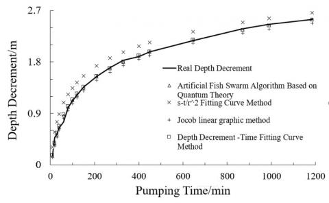
With the QAFSA, we can calculate the water transmissibility coefficient, the water storage coefficient, the objective function value, as well as the average relative error and the maximum relative error between the measured value and the calculated value, see Table 2 for details. The average relative error value and the objective function value calculated by the QAFSA were smaller than those of the traditional methods, so the calculated results of the proposed method were higher in accuracy and credibility. As shown in Figure 1, after the parameters T and S which had been obtained via inversion of the intelligence algorithm were substituted into Formula (5), the calculated water depth decrement value was closer to the measured water depth decrement value.
Table 2. Comparison of the calculation results of several methods
|
methods |
S/(10-4) |
T/(m2·d-1) |
E/(10-3) |
average relative error/% |
|
s-t/r2 Fitting Curve Method |
1.47 |
212.30 |
35.26 |
20.9 |
|
Depth Decrement -Time Fitting Curve Method |
2.38 |
197.67 |
1.75 |
4.0 |
|
Jocob linear graphic method |
2.78 |
194.00 |
4.97 |
7.0 |
|
Artificial Fish Swarm Algorithm Based on Quantum Theory |
2.50 |
193.20 |
1.39 |
3.1 |
Figure 1. Comparison of the measured and calculated values of several methods
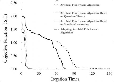
AFSA can invert the parameters of aquifer with high efficiency, and it has good global convergence. However, when the AF enters the optimum solution space for optimization, AFSA is limited due to factors such as step or visual, resulting in multiple calculation results oscillating back and forth around the extreme values, and the solution accuracy is relatively low. The proposed QAFSA was compared with the SA-based (simulated annealing) AFSA and the adaptive AFSA proposed by literatures [13] and [14], the calculation results are shown in Table 3 and the convergence curve is shown in Figure 2.
Table 3. Comparison of the calculation results of several AFSAs
|
methods |
converging iterations |
E/(10-3) |
average relative error /% |
|
Artificial Fish Swarm Algorithm |
132 |
8.34 |
7.7 |
|
Adapting Artificial Fish Swarm Algorithm |
28 |
1.59 |
5.8 |
|
Artificial Fish Swarm Algorithm Based on Simulated Annealing |
76 |
1.19 |
2.7 |
|
Artificial Fish Swarm Algorithm Based on Quantum Theory |
37 |
1.39 |
3.1 |
Figure 2. Convergence curve of the objective function
(1) Comparison between the QAFSA and adaptive AFSA
For the QAFSA and adaptive AFSA, when searching for optimum solution in the solution space, both adopt variable step and visual to perform the searching, therefore, during aquifer parameter inversion, both algorithms have fast convergence speed. The difference is, when applying adaptive AFSA for algorithm optimization, the change of step and visual are related to the distance between current AF and the optimum AF, or are set to be simply negatively correlated with the number of iterations that have been performed so far. The optimization method is relatively simple and the step and visual of AF are larger than those of the QAFSA. Moreover, the QAFSA adopts QRG for AF updating, during which the size of the rotation angle is determined by the adaptive step strategy, and the rotation direction is determined by the theorem in literature [15], therefore, when the QAFSA performs optimum solution searching, the algorithm is even more complicated. During inversion, the step and visual of AF are smaller, so its convergence speed is slightly slower than that of the adaptive AFSA, but its solution accuracy is improved by about 13 % compared with the adaptive AFSA.
(2) Comparison between the QAFSA and SA-based AFSA
SA-based AFSA first uses AFSA to optimize the objective function, after a certain number of iterations, it outputs current optimum value and takes it as the initial value of SA to continue the searching for the optimum solution. This algorithm makes full use of the global searching ability of AFSA and the powerful local searching ability of SA. Therefore, when this algorithm is applied for the inversion of aquifer parameters, the value of objective function is the smallest, and the relative error between the calculated value and the measured value is the smallest. However, in practical application, it still has a few limitations, for instance: How to properly allocate the number of iterations of AFSA and SA, especially the setting of iteration number of AFSA, if the number is set too small, then the output result is not necessarily a point in the extreme value region, moreover, if it’s taken as the initial value for SA, as a result, the accuracy of the calculation result often cannot truly reflect the parameters of the aquifer; otherwise, if the number is set too large, even if the accuracy of the hybrid algorithm is guaranteed, the time consumption will be multiplied, especially when it’s applied to the inversion of aquifer parameters of a well cluster, the difference in calculation time is particularly obvious. On the contrary, when being applied to single well water pumping test or well cluster water pumping test, the QAFSA only needs a preset termination criterion to give more convenient and faster results on the condition that the accuracy of the solution is guaranteed.
The QAFSA applies qubit coding for AF and uses QRG to update its status, so that the AF can simulate the fish swarm’s four behaviors such as preying, the proposed algorithm has the advantages of strong global searching ability, high solution accuracy, and fast convergence speed, etc., by comparing its pros and cons with other algorithms, following conclusions are drawn:
(1) The QAFSA can accurately invert the aquifer parameters, and its inversion accuracy is far better than that of the traditional methods, so it can be applied to the solution of the geological parameter water level.
(2) Compared with adaptive AFSA, the QAFSA not only retains the merit of fast convergence when using variable step and visual for searching, but also improves the solution accuracy by about 13 %; Moreover, compared with SA-based AFSA, the QAFSA doesn’t have to consider the setting of iteration number and its influence on the solution results, which makes the algorithm have a faster convergence speed while ensuring accuracy. Weighing the influence of solution accuracy, convergence speed, and other indicators, it’s concluded that the QAFSA has a better application value.