Nurru Anida Ibrahim![]() | Arunkumar Subramaniam
| Arunkumar Subramaniam![]() | Siti Norbakyah Jabar
| Siti Norbakyah Jabar![]() | Salisa Abdul Rahman*
| Salisa Abdul Rahman*![]()
© 2024 The authors. This article is published by IIETA and is licensed under the CC BY 4.0 license (http://creativecommons.org/licenses/by/4.0/).
OPEN ACCESS
This research article presents a comprehensive comparative analysis of driving patterns in Kuala Terengganu during various peak hours, shedding light on the dynamic nature of urban traffic flows. The study aims to provide valuable insights into the temporal variations in vehicular behaviour within this Malaysian city, with the ultimate goal of informing transportation planning and policy decisions. To achieve this objective, a diverse dataset of vehicle trajectories, collected through GPS tracking systems, was meticulously analysed. The data encompassed two different peak hours, including morning and evening peaks which is go-to-work time and back-from-work time. Several key parameters such as speed, acceleration, deceleration, and others were meticulously extracted and statistically compared across different timeframes. The findings of this study reveal striking disparities in driving behaviour during distinct peak hours. Evening peak hours, characterized by rush hour congestion, displayed significantly lower average speeds, higher traffic density, and increased instances of abrupt acceleration and deceleration. In contrast, morning peaks exhibited more fluid traffic conditions with higher average speeds and reduced congestion. This research provides a comprehensive understanding of the nuances of driving patterns in Kuala Terengganu, shedding light on the temporal dynamics of urban traffic. Finally, the insights generated by this comparative study could be useful for urban planners, traffic control bodies, and policy-makers to minimize peak-hour traffic by using the existing transportation infrastructure more effectively. Moreover, the methodology followed in this research could be useful as a model study approach for similar research in other urban areas, resulting in normalized and efficient urban transportation.
driving cycle, driver’s behavior, fuel economy, emissions, hybrid electric vehicles
From a conceptual standpoint, the term "local driving pattern" refers to the typical driving traits found in the area. Driving patterns, according to Desineedi et al. [1], are commonly represented by a speed-time series, which is termed a driving cycle. As discussed in the study [2-5], “a driving cycle is a predetermined speed-time macrograph that shows the driving habits of a certain area or city”. This is a list of the operating modes for a vehicle, including idle, accelerate, cruise, and decelerate. Even so, because different cities have different topographies, vehicle types under consideration, vehicle compositions, and road types, operating circumstances may differ among cities [6, 7]. In order to comprehend and predict the driving habits, emissions, and energy consumption of various vehicle types, researchers and practicing engineers frequently utilise driving cycles [8]. Driving cycles explain the stresses put on cars and have thus been used to measure the environmental impact of traffic [9], as well as to optimise the powertrain configurations and engine control systems of new vehicles to reduce fuel consumption [10].
During the process of regulatory approval for new vehicle technologies, manufacturers and environmental agencies predominantly utilize driving patterns to evaluate the efficiency of fuel consumption and the release of pollutants from vehicles [11]. When these patterns are employed for regulatory purposes, they are known as type-approval driving cycles [12]. Presently, manufacturers commonly rely on specific type-approval driving cycles such as the Federal Test Procedure (FTP) 75, Urban Dynamometer Driving Schedule (UDDS), New European Driving Cycle (NEDC), and Worldwide harmonised Light vehicles Test Cycles (WLTC) to report the fuel consumption and emissions of their vehicles [13].
Hence, this scholarly article offers an extensive comparative examination of driving cycles observed in Kuala Terengganu during different peak periods. Additionally, it delves into the creation of a driving cycle specific to Kuala Terengganu using the MATLAB Mobile application, focusing on two distinct peak hours. Subsequently, the study will assess energy usage and emissions through the utilization of AUTONOMIE software.
This section will cover a few of the ongoing initiatives and past studies that both directly and indirectly support and contribute to the accomplishment and success of this research.
2.1 Route selection
Choosing a route is a crucial step in creating a driving cycle. In an urban environment, traffic jam is perceived to differ with the route and time of the day. One can expect regular weekday, week harsh hours stereotypically have worse traffic jams than off-peak hours and weekends and public deficit days [14]. The pattern selected should be retrieved from the real route layout in the research area and consider the causes of traffic volume encountered including road power, topography, intersections, demographic density, slope, and weather factor [15]. The actual circumstances that arise along each route must be located and determined before the routes are chosen [16]. The routes that were selected must have the following characteristics: heavy traffic; connecting important population centres; high emissions on the transit route; a variety of squares and crossroads; and availability of public transportation [17].
Research is carried out on them due to the fact that the researchers have an understanding of local conditions. At the same time, many scholars have developed a methodology. Specifically, before determining the distance of every chosen route, Zhao et al. [18] used ArcGIS software to analyse the topological structure of Xi’an urban highways. They also collected information on many sample roads and continued to record recording points in turn and observe the traffic volume during peak and off-peak hours [18]. The authors of the study recorded four categories of traffic in Delhi, DC: congested, semi-urban, urban, and extra-urban [19].
2.2 Data collection
The data collection process can begin after the representative routes have been chosen. The terms "car chasing technique" and "on-board measurement technique" refer to two distinct methods for gathering data. It is also possible to collect data using a hybrid method strategy, which combines the two ways mentioned above.
The on-board measuring approach involves installing an instrument in a specific vehicle and allowing it to move along a predetermined route or traffic stream. Then, as they follow the pre-planned itineraries, second-by-second speed data is captured. This approach works well in nations whose driving behaviour is erratic and combative. Additionally, for the nations that have databases pertaining to traffic to precisely choose the routes. For instance, real-world data for the Tehran driving cycle was gathered using the on-board measurement approach, in which an Advanced Vehicle Location (AVL) device was installed in the car and used for six months to collect data along various routes in Tehran [9]. Based on GPS technology, the AVL is an advanced vehicle tracking and monitoring gadget. The China Light-duty vehicle Test Cycle (CLTC), created by Liu et al., also made use of an on-board measurement method that sent real-time signals to the CATC information system via the General Packet Radio Service (GPRS) network. This method used the vehicle's Global Positioning System (GPS) signal and parameters related to on-board diagnostics (OBD) using a unified data protocol [20]. Using a high-end GPS data recorder, 100 e-rickshaw excursions are recorded over a road segment that passes through both rural and urban settings in another study established by Chandrashekar et al. [21].
In contrast, a target vehicle is pursued in a pre-set route or routes within an area of concern by an instrumented vehicle that has the capability to measure speed data on a second-by-second basis [2]. In order to get correct data, drivers must follow the target vehicle exactly as it goes. This technique is particularly challenging on routes with low line-of-sight (LOS). Chase-car strategy was utilised on twelve routes, including urban and highway routes, in the driving cycle established in Kuala Lumpur by Tharvin et al. [22]. Before beginning the data collection, every piece of equipment was calibrated. According to Saleh et al., the driving cycle established in Edinburgh collected data on driving cycles along six major roads and five radials that were connected to them using the chase car method [23]. Pune driving cycle in India uses a similar technique that entails selecting a vehicle at random from the traffic and having the survey vehicle just follow it while maintaining a roughly constant distance during various modes of operation [24]. As evaluated by Ho et al. [25], real-world driving cycles that are directly produced from the chase-car method include the driving cycles in Bangkok, Hong Kong, Sydney, and LA-92.
2.3 Driving cycle development
Cycle construction approaches typically involve the following steps: Real-world driving data gathering is the first step, followed by segmentation, cycle construction, evaluation, and final cycle selection [26]. There is not a single, recognised method for developing a driving cycle. Various agencies, authorities, and scholars might create their own driving cycles for a variety of uses, such analysing fuel efficiency, testing emissions, or evaluating car performance. Various methodologies, including constructing cycles based on micro-trips, segment-based approaches, pattern classification, and modal cycle development, are utilized to create driving patterns from collected data [27, 28].
Pune’s driving cycle, a major city in India, using micro-trips taken from actual driving data. The driving cycle development incorporated factors such as time-space profiles, percentage of acceleration/deceleration, idle periods, duration of cruising, and average speed to more accurately reflect typical traffic scenarios found in large and busy city [24]. Segment-based cycle construction, akin to micro-trip-based methods, is unsuitable for traffic conditions characterized by frequent stops and is contingent upon road type and traffic flow [2]. This approach makes the greatest sense when used for a driving cycle in traffic design, but it is not appropriate for emission control as the trip fragments can accurately depict both the real traffic situation and the physical features of the road and LOS. In Chennai, another important Indian metropolis, the study created a distance-based driving cycle designed for intra-city buses. This created driving cycle was then contrasted with many standard driving cycles [29].
Several well-known methods, such as Markov chain theory, clustering approaches, random and quasi-random micro-trip selection, and random selection of micro-trips, are utilised in the design of the driving cycle. Micro-trip selection in the quasi-random approach is an incremental process that keeps going until the target driving cycle time is reached. In contrast with random selection, the quasi-random selection method for driving cycles involves identifying the optimal cycle by aligning it with the speed acceleration frequency distribution (SAFD) observed across the whole dataset [30]. However, a notable drawback of the quasi-random selection of micro-trips is its inability to precisely capture the modal activities in terms of their frequency, duration, and intensity.
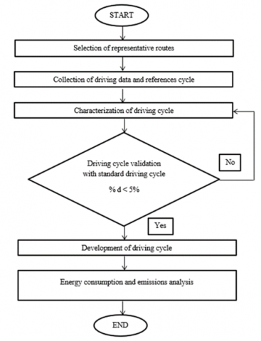
Several key tasks must be addressed to finalize this project, including selecting routes for developing the KT driving cycle, determining the method for data collection, and creating a driving cycle using the k-means approach during two distinct peak periods. Subsequently, the paper will delve into analysing energy consumption and emissions of developed driving cycle. The study flow map for creating a driving cycle in KT during rush hour and after work along five distinct routes is displayed in Figure 1.
Figure 1. Flow chart of the study
3.1 Route selection and data collection
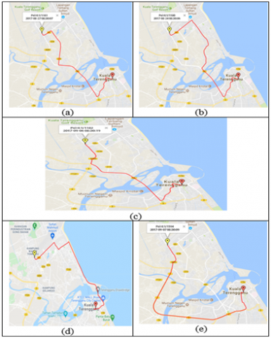
Establishing the representative routes across the region of interest is the most crucial step in creating the driving cycle. Data collection for the KT drive cycle will take place on both suburban and urban roads. The pathways from Kampung Gong Badak to Terengganu's Wisma Persekutuan are included in this project. Figure 2 shows the five main roads—Route A–E—that connect Kampung Wakaf Tembesu to Wisma Persekutuan [31]. These routes were obtained from Google Maps. These five routes are the most often utilised "route-to-work" routes by KT citizens, according to the Road Traffic Volume Malaysia 2019 (RTVM) report provided by Ministry of Works Malaysia [32]. As in the report, Kuala Terengganu’s Road traffic volume is displayed in Table 1. As indicated in Table 1, LOS is a descriptive statistic which describes the speed, duration of travel, manoeuvrability, comfort, convenience, interruption of traffic, and safety of the traffic circumstances. The optimal situation is represented by LOS A, whereas highly crowded traffic with demands for more space on the roadway are represented by LOS F. All five chosen routes are categorized in LOS F.
Figure 2. Five chosen routes, (a) Route A; (b) Route B; (c) Route C; (d) Route D; and (e) Route E
Table 1. Average road traffic volume in KT for 2019
|
Census Station No. |
16-hour Traffic |
Peak Hour Traffic |
Traffic Composition (%) |
||||||
|
Cars & Taxis |
Vans & Utilities |
Medium Lorries |
Heavy Lorries |
Buses |
Motor |
LOS |
|||
|
TR401 |
21665 |
1999 |
53.1 |
17.6 |
5.0 |
2.3 |
0.6 |
21.4 |
F |
|
TR404 |
11087 |
1139 |
70.0 |
10.5 |
3.4 |
0.9 |
0.7 |
14.5 |
A |
|
TR405 |
67928 |
7376 |
68.0 |
7.8 |
2.1 |
0.6 |
0.3 |
21.2 |
F |
|
TR406 |
20067 |
2159 |
50.5 |
9.4 |
5.8 |
1.6 |
0.2 |
32.4 |
F |
|
TR409 |
30842 |
3731 |
54.9 |
5.4 |
5.2 |
1.3 |
0.3 |
33.0 |
F |
Throughout the designated route, it is imperative to track the vehicle's speed over time. Data collection along this route will occur during the peak commuting hours of 7:30 to 8:30 a.m. Furthermore, data will be collected during the busiest return-from-work periods between 4:30 to 5:30 p.m. For each time slot, ten runs will be recorded, resulting in a total of 300 speed data points. The on-board measurement method will be used for data collection for the KT driving cycle, given its suitability for capturing the erratic driving behaviours typical of KT drivers, who must navigate safely amidst unpredictable occurrences such as accidents and incidents. GPS and data loggers will serve as the data collection tools for this purpose.
The Apple iPhone SE second generation running iOS 15 was utilised for data gathering purposes for the duration of this study. The utilization of an iPhone has demonstrated itself as a viable substitute for expensive vehicle tracking devices when employed in a probe vehicle, showcasing comparable accuracy levels [33]. Notably, its positioning capabilities have proven highly reliable and consistent, particularly in open sky environments. The precision achieved is also sensitive and valuable for depicting vehicle dynamics and recognizing manoeuvres. Consequently, it is anticipated that the iPhone SE utilized in the present study would maintain, if not surpass, similar levels of accuracy, given advancements in hardware components.
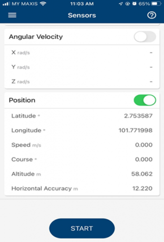
The MATLAB Mobile programme, which is loaded on a mobile phone and connected to the car during the data collecting procedure, is the instrument utilised in this research to gather data. For mobile devices, the MATLAB Mobile application is a small desktop that links to MATLAB sessions that are operating on desktops or the Math Works Computing Cloud [34]. As seen in Figure 3, the GPS-enabled data in the MATLAB mobile application will be immediately uploaded to the MATLAB cloud database.
Figure 3. The GPS sensor in the MATLAB mobile application
The researcher used only one type of car and the same driver throughout the collection process to avoid inconsistency of the data. The car used throughout this research was Perodua Myvi 1.3 EZi (2010). Throughout the data collection process, the researcher carried the device inconspicuously as a regular passenger to prevent any influence on the driver. Following the removal of abnormal data, the collected data is segmented into kinematic sequences.
3.2 Characterization of KT driving cycle
After the data collection process, the data is uploaded and stored in the MATLAB drive cloud. The application allows for quick validation of the driving cycle assessment of the driving data. An essential part of characterising and validating the driving cycle is a cycle assessment.
Table 2 presents the formula to compute each parameter within the KT driving cycle. These nine parameters have been selected as they form the fundamental criteria for evaluation and are widely employed to characterize the driving cycle.
Table 2. The assessment parameters and its formula
|
Parameters |
Unit |
Formula |
|
Average speed of whole driving cycle, V1 |
Km/h |
V1 = 3.6 $\frac{\text { dist }}{\mathrm{T}_{\text {total }}}$ |
|
Average running speed, V2 |
Km/h |
V2 = 3.6 $\frac{\text { dist }}{\mathrm{T}_{\text {drive }}}$ |
|
Average acceleration of all acceleration phase, a |
m/s2 |
$\begin{gathered}a= \\ \left(\sum_{i=1}^n\left\{\begin{array}{cc}1 & \left(a_i>0\right) \\ 0 & (\text { else })\end{array}\right)-1\right. \\ \left(\sum_{i=1}^n\left\{\begin{array}{cc}a_i & \left(a_i>0\right) \\ 0 & (\text { else })\end{array}\right)\right.\end{gathered}$ |
|
Average deceleration of all deceleration phase, d |
m/s2 |
$\begin{aligned} & d= \\ & \left(\sum_{i=1}^n\left\{\begin{array}{cc}1 & \left(a_i<0\right) \\ 0 & (e l s e)\end{array}\right)^{-1}\right. \\ & \left(\sum_{i=1}^n\left(\begin{array}{cc}a_i & \left(a_i<0\right) \\ 0 & (e l s e)\end{array}\right)\right. \\ & \end{aligned}$ |
|
Root mean square acceleration, RMS |
m/s2 |
RMS = $\sqrt{\frac{1}{T} \int_0^T(a)^2 d t}$ |
|
Percentage idling Pi, v(t) = 0 km/h |
% |
- |
|
Acceleration Pa, v(t) $\geq$3 km/h, a(t) $\geq$ 0.1 m/s2 |
% |
% acc = $\frac{\mathrm{T}_{\text {acc }}}{\mathrm{T}_{\text {total }}}$ |
|
Cruising Pc, v(t) $\geq$ 3 km/h, -0.1 $\leq a(t)<0.1$ m/s2 |
% |
% cruise = $\frac{\mathrm{T}_{\text {cruise }}}{\mathrm{T}_{\text {total }}}$ |
|
Deceleration Pd, v(t) $\geq$ 3 km/h, a(t) $<$ -0.1 m/s2 |
% |
% dec = $\frac{\mathrm{T}_{\text {dec }}}{\mathrm{T}_{\text {total }}}$ |
3.3 Kuala Terengganu driving cycle development
The driving cycle has been proposed to be created through clustering of micro-trips. The distance travelled in a vehicle while maintaining a steady speed is known as a micro-trip [35]. Each micro-trip consists of an end phase, a decreasing deceleration phase, and an idle interval. The entire process of collecting data needs to be divided into multiple short journeys. When this procedure is complete, a significant number of micro-trips for the total amount of data collected can be obtained. Based on the intensity of the traffic flow, the micro-trips are then categorised as heavy, medium, or light traffic. The micro-trips will be grouped using the k-means method.
A popular unsupervised machine learning technique for clustering or assembling similar data points is k-means clustering. K-means clustering is an unsupervised learning method that does not require labelled data or prior knowledge of the groupings. because it is flexible and may be used with a range of driving datasets without the need for human annotation. K-means clustering can handle large datasets with plenty of features and data points since it is computationally efficient. It scales effectively and can process big amounts of driving data in a fair amount of time. Each data point will be assigned to the cluster with the closest mean value once a dataset has been separated into k distinct clusters [36].
First, all driving data is cleaned and pre-processed to ensure that the data obtained is in a format suitable for the k-means method. This step may involve filling in any missing values, standardising or normalising the data, and eliminating outliers from the sample. Second, it is decided which relevant features or parameters will be used to define the driving cycle patterns. Since they will have the biggest impact on emissions, average speed and percentage idle values are two examples of typical driving cycle characteristics [9]. After that, a driving cycle is constructed by selecting the value of k. There is flexibility in changing the number of clusters, k, to meet specific needs or objectives. By choosing the appropriate k number, the driving cycle can be modified to record different granularities in the driving patterns, allowing for more intricate analysis or optimisation. The value of k is set to three for this project, taking into account three possible traffic scenarios. Every cluster's centroid values are initialised at random. These centroids represent the mean values of the data points assigned to each cluster. By iteratively walking over the dataset, each data point is assigned to the cluster with the closest centroid. Using a distance metric, usually the Euclidean distance (RN), this phase calculates the similarity between each cluster centroid and the data point [37]. Clustering within an N-dimensional Euclidean space, denoted as RN, involves dividing a given set of n points into a specified number, denoted as K, of groups based on a similarity or dissimilarity metric. Let the set of n points {x1, x2, …, xn} be denoted by set S, and let K clusters be represented by C1, C2, …., Ck. Then:
Each cluster Ci is not empty for every i = 1, …, K. The intersection of any two clusters Ci and Cj is empty for every i = 1, …, K and j = 1, …, K where i ≠ j, and:
$U_{i=1}^K C_i=S$ (1)
To recalculate the centroids of each cluster, the mean of all the data points assigned to that cluster is found. Until convergence is reached, the centroid update and assignment procedures are repeated. Convergence occurs when either the maximum number of iterations is reached or the centroids show no more appreciable change. Upon convergence of the algorithm, the resultant clusters undergo analysis and investigation. To do this, it could be required to examine each cluster's characteristics, visualise the driving patterns within each cluster, and then use domain knowledge or specific objectives to interpret the results.
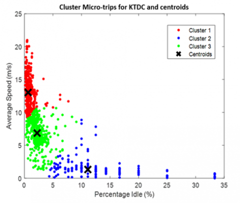
Minimising the sum of squared distances between each data point and its assigned centroid is the algorithm's main objective. To do this, data points are distributed iteratively, and centroids are updated until convergence. The outcome is a collection of k clusters, each of which has a centroid to represent it. The clusters are then assigned data points according to how far away from the centroids the data points are. As seen in Figure 4, the micro-trips are split into three groups using the k-means clustering technique. Each category represents a particular traffic condition (heavy, medium, or clear) and has unique qualities.
Figure 4. Clustering of the micro-trips
The KT driving cycle is created using the k-means approach based on go-to-work times, which are at 7.30, 8.00, and 8.30 a.m., as was previously covered in the previous section. Additionally, around the times when employees return from work—4.30, 5.00, and 5.30 p.m. Every route presents a unique driving cycle pattern, as seen in the Figure 5 and Figure 6 for each driving cycle. This can be attributed to various external factors, including traffic signals, road conditions, driving habits, and surrounding circumstances.
4.1 Kuala Terengganu driving cycle at go-to-work time
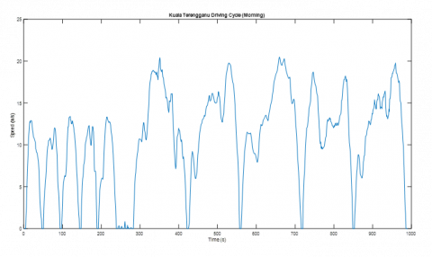
Figure 5 shows the KTDC along Routes A to E, at 7.30 to 8.30 a.m. when the value of k is 3, representing three different traffic groups: congested, medium, and clear. The total number of final micro-trips is 15, and the total time taken to complete the cycle is 990 seconds. Table 3 presents a tabulation of KTDC's attributes based on nine assessment categories.
It is evident from all of the numbers and the table that the speed range above 36 km/h dominated. This demonstrates that, in contrast to large, cosmopolitan cities like Kuala Lumpur, the traffic flow in Kuala Terengganu city is not overly congested, even though the data was collected at peak hour [37]. Greater speed ranges result in lengthier micro-trips than lesser speed ranges. This is so that a car in a free flow can go faster and stop less often when there is less traffic. The developed KT driving cycle's observed average speed of 39.14 km/h suggests a slower rate of vehicle movement and suggests that there are more micro-trips occurring below this average speed. This slower pace corresponds to heightened fuel consumption and emissions during this period, attributed to the frequent stops encountered throughout the journey.
Figure 5. Kuala Terengganu driving cycle at go-to-work time
Figure 6. Kuala Terengganu driving cycle at back-from-work time
Table 3. Assessment parameters of KT driving cycle at go-to-work time
|
Parameters |
KTDC (Morning) |
|
Distance travelled (km) |
10.76 |
|
Total time (s) |
990 |
|
Average speed (km/h) |
39.14 |
|
Average running speed (km/h) |
42.58 |
|
Average acceleration (m/s2) |
0.46 |
|
Average deceleration (m/s2) |
0.50 |
|
RMS (m/s2) |
0.63 |
|
Percentage idle (%) |
6.57 |
|
Percentage cruise (%) |
0.71 |
|
Percentage acceleration (%) |
48.59 |
|
Percentage deceleration (%) |
44.14 |
Table 4. Assessment parameters of KT driving cycle at back-from-work time
|
Parameters |
KTDC (Evening) |
|
Distance travelled (km) |
9.61 |
|
Total time (s) |
897 |
|
Average speed (km/h) |
38.56 |
|
Average running speed (km/h) |
41.58 |
|
Average acceleration (m/s2) |
0.48 |
|
Average deceleration (m/s2) |
0.53 |
|
RMS (m/s2) |
0.68 |
|
Percentage idle (%) |
5.91 |
|
Percentage cruise (%) |
1.23 |
|
Percentage acceleration (%) |
48.72 |
|
Percentage deceleration (%) |
44.15 |
4.2 Kuala Terengganu driving cycle at back-from-work time
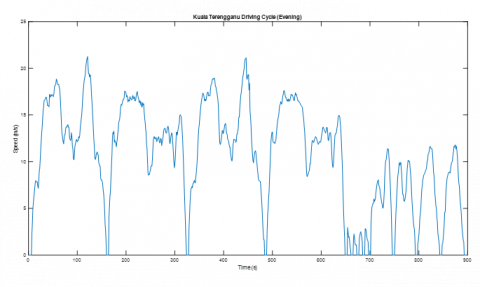
Figure 6 depicts the KTDC along Routes A to E during evening peak hours when k equals 3, representing three traffic groups: congested, medium, and clear. The total number of final micro-trips is 12, and the cycle takes 897 seconds to complete. Table 4 summarizes the features of KTDC in terms of nine assessment parameters.
The speed range above 25 km/h was dominant, as can be seen in the figures and table. This demonstrates that there is more traffic during the evening peak hour than there is during the morning peak hour. In comparison to morning peak hour, the developed KT driving cycle’s average speed of 38.56 km/h indicates that cars are travelling more slowly and that there are more micro-trips made at slower speeds. During evening peak hour, there are more pollutants and fuel consumption due to the numerous stops along the road.
4.3 Comparative analysis of KTDC assessment parameters with standard driving cycles
Table 5. Comparison of KTDC and standard driving cycles
|
Parameters |
KTDC (PM) |
KTDC (AM) |
NEDC |
UDDS |
LA-92 |
|
Distance travelled (km) |
9.61 |
10.76 |
11.02 |
12.89 |
15.80 |
|
Total time (s) |
897 |
990 |
1180 |
600 |
1436 |
|
Average speed (km/h) |
38.56 |
39.14 |
33.6 |
31.51 |
39.4 |
|
Average running speed (km/h) |
41.58 |
42.58 |
42.24 |
38.85 |
47.0 |
|
Average acceleration (m/s2) |
0.48 |
0.46 |
0.53 |
0.50 |
0.67 |
|
Average deceleration (m/s2) |
0.53 |
0.50 |
0.72 |
0.58 |
0.75 |
|
RMS (m/s2) |
0.68 |
0.63 |
0.14 |
0.68 |
0.79 |
|
Percentage idle (%) |
5.91 |
6.57 |
16.95 |
17.66 |
15.1 |
|
Percentage cruise (%) |
1.23 |
0.71 |
38.81 |
7.96 |
12.5 |
|
Percentage acceleration (%) |
48.72 |
48.59 |
23.56 |
39.71 |
38.3 |
|
Percentage deceleration (%) |
44.15 |
44.14 |
17.29 |
34.67 |
34.1 |
To assess the KTDC that was formulated, a comparison was conducted with various international peak-hour cycles outlined in Table 5. Specifically, the driving cycle designed for passenger vehicles was juxtaposed with the Unified Cycle Driving Schedule Test Procedure (LA-92) driving cycle, which was initially devised for emission-related objectives. Besides, the NEDC and the UDDS, two current standard driving cycles, are compared to the KTDC in Table 5. The selection of NEDC for comparison with KTDC stems from its continued utilization in Malaysia for regulatory purposes by the local authorities, as well as by domestic manufacturers and suppliers for assessment purposes [37]. Similarly, UDDS was chosen for comparison due to its tailored design for urban driving scenarios and its relevance for emission evaluation.
The table presents a comprehensive comparison of several driving cycles, including Kuala Terengganu driving cycles during morning and evening peak hours (KTDC AM and KTDC PM), along with NEDC, UDDS, and LA-92. Various parameters are evaluated to understand the characteristics of each driving cycle. Firstly, in terms of distance traveled, LA-92 stands out with the longest distance covered at 15.80 km, while KTDC (PM) covers the least distance at 9.61 km. Regarding total time taken, UDDS demonstrates the shortest duration of 600 seconds, whereas LA-92 requires the most time at 1436 seconds. The average speed maintained during the cycles varies, with KTDC (AM) exhibiting the highest average speed at 39.14 km/h, and NEDC showing the lowest at 33.6 km/h. Additionally, average acceleration and deceleration rates provide insights into driving behavior, with LA-92 displaying the highest values for both parameters. Percentage metrics such as idle time, cruise time, acceleration time, and deceleration time shed light on driving patterns. Notably, NEDC shows a significant portion of cruise time at 38.81%, while KTDC (PM) and KTDC (AM) exhibit the highest percentages of acceleration and deceleration time. Overall, each driving cycle presents unique characteristics, which can be instrumental in analyzing fuel efficiency, emissions, and overall vehicle performance under different driving conditions.
4.4 Kuala Terengganu driving cycle fuel rate and emissions analysis
The fuel rate, including fuel consumption and fuel economy, also emissions, can be assessed using AUTONOMIE software version v1210 once the driving cycle has been formulated. AUTONOMIE serves as a software tool utilized for the design, simulation, and analysis of automotive control systems. This software relies on mathematical principles for forward simulation and operates within the MATLAB environment, utilizing MATLAB data, configuration files, and models integrated into Simulink. The findings of the KT driving cycle fuel rate and emission analysis using a PHEV powertrain are displayed in Table 6 and were taken from AUTONOMIE software. As indicated in the table, the outcomes illustrate that the powertrain performs satisfactorily in mitigating excessive fuel consumption and, consequently, curbing the escalation of air pollution within KT city.
When contrasting the morning and evening peak hours, the data in the table illustrates that the morning peak hour exhibits lower fuel consumption and emissions due to relatively lighter traffic congestion compared to the evening peak hour. This results in the morning peak hour showcasing the lowest levels of fuel consumption and emissions, alongside the highest fuel economy. Conversely, the evening peak hour experiences higher emissions and fuel consumption, attributed to frequent stops along the road. The percentage difference in fuel economy between KTDC at go-to-work time and KTDC at back-from-work time is 5.73%. While the percentage difference of fuel consumption and emissions is 6.06% and 20.51%, respectively.
Table 7 and Table 8 in the other hand show the fuel rate and emissions of KT driving cycle using conventional engine vehicles, hybrid electric vehicle (HEV) and PHEV. As in the tables, the reduction percentage of fuel consumption and CO emission between PHEV and HEV is 7.27% for KTDC at go-to-work time and 5.48% for KTDC at back-from-work time. While the reduction percentage of fuel consumption and CO emission between PHEV and conventional vehicle is 10.82% using KTDC at go-to-work time and 9.33% difference when using KTDC at back-from-work time.
Table 6. Fuel rate and emissions analysis of KT driving cycle
|
Parameters |
KTDC (Morning) |
KTDC (Evening) |
|
Fuel economy (km/l) |
20.66 |
19.51 |
|
Fuel consumption (l/100km) |
4.8 |
5.1 |
|
CO emissions (g/km) |
0.862 |
1.059 |
Table 7. Comparison of different vehicle powertrain using KTDC (AM)
|
Parameters |
PHEV |
HEV |
Conv |
|
Fuel economy (km/l) |
20.66 |
19.21 |
18.54 |
|
Fuel consumption (l/100km) |
4.8 |
5.1 |
5.4 |
|
CO emissions (g/km) |
0.862 |
0.957 |
1.589 |
Table 8. Comparison of different vehicle powertrain using KTDC (PM)
|
Parameters |
PHEV |
HEV |
Conv |
|
Fuel economy (km/l) |
19.51 |
18.47 |
17.77 |
|
Fuel consumption (l/100km) |
5.1 |
5.24 |
5.6 |
|
CO emissions (g/km) |
1.059 |
2.116 |
3.083 |
The study successfully achieved its objectives of constructing a driving cycle in KT city using k-means clustering during different peak hours which is morning and evening peak hour. The methodology combined micro-trips-based and pattern classification approaches, resulting in a comprehensive representation of traffic behaviours. The created KT driving cycle was validated and compared with existing driving cycles, demonstrating its effectiveness with fifteen micro-trips and an average speed of 38.56 km/h and 39.14 km/h. From the energy consumption and emission analysis using AUTONOMIE software, it can be concluded that PHEV gives the best result compared to HEV and conventional engine vehicle with reduction of 65.49% and 82.06%, respectively. By analysing and contrasting driving behaviours and traffic conditions during various times of the day, this research has shed light on the potential for optimizing transportation strategies and infrastructure development to alleviate congestion and enhance the overall driving experience in Kuala Terengganu. The findings of this study can serve as a foundation for future urban planning and traffic management efforts, ultimately contributing to a more sustainable and efficient transportation system in the city.
For future research, it is recommended to broaden the scope of data collection to encompass a wider range of Malaysian driving behaviors, including various states, road types, and vehicle categories. Specialized driving cycles tailored to Malaysia's unique driving conditions, such as urban congestion, hilly terrain, and tropical weather, should be developed to accurately represent the country's driving scenarios.
The data utilized in this research can be obtained upon request via the Faculty of Ocean Engineering Technology's institutional account. Authors have provided a link for data access.
The authors would like to be obliged to Universiti Malaysia Terengganu for providing financial assistance under FRGS 2020-1 (Grant numbers: FRGS/1/2020/TK0/UMT/02/2) and Faculty of Ocean Engineering Technology, UMT for all their technical and research support for this work to be successfully completed.
[1] Desineedi, R.M., Mahesh S., Ramadurai G. (2020). Developing driving cycles using k-means clustering and determining their optimal duration. Transportation Research Procedia, 48: 2083-2095. https://doi.org/10.1016/j.trpro.2020.08.268
[2] Galgamuwa, U., Perera, L., Bandara, S. (2015). Developing a general methodology for driving cycle construction: Comparison of various established driving cycles in the world to propose a general approach. Journal of Transportation Technologies, 5(4): 191-203. http://doi.org/10.4236/jtts.2015.54018
[3] Tong, H.Y., Ng, K.W. (2021). Development of bus driving cycles using a cost effective data collection approach. Sustainable Cities and Society, 69: 102854. https://doi.org/10.1016/j.scs.2021.102854
[4] Tong, H.Y., Ng, K.W. (2021). A bottom-up clustering approach to identify bus driving patterns and to develop bus driving cycles for Hong Kong. Environmental Science and Pollution Research, 28: 14343-14357. https://doi.org/10.1007/s11356-020-11554-w
[5] Liu, Y., Wu, Z.X., Zhou, H., Yu, H.Z.N., An, X.P., Li, J.Y., Li, M.L. (2020). Development of China light-duty vehicle test cycle. International Journal of Automotive Technology, 21: 1233-1246. http://doi.org/10.1007/s12239-020-0117-5
[6] Liu, H., Zhao, J.Y., Qing, T., Li, X.Y., Wang, Z.Z. (2021). Energy consumption analysis of a parallel PHEV with different configurations based on a typical driving cycle. Energy Reports, 7: 254-265. https://doi.org/10.1016/j.egyr.2020.12.036
[7] Jia, X.Y., Wang, H.W., Xu, L.F., Wang, Q., Li, H., Hu, Z.Y., Li, J.Q., Ouyang, M.G. (2021). Constructing representative driving cycle for heavy duty vehicle based on Markov chain method considering road slope. Energy and AI, 6: 100115. https://doi.org/10.1016/j.egyai.2021.100115
[8] Borlaug, B., Holden, J., Wood, E., Lee, B., Fink, J., Agnew, S., Lustbader, J. (2020). Estimating region-specific fuel economy in the United States from real-world driving cycles. Transportation Research Part D: Transport and Environment, 86: 102448. https://doi.org/10.1016/j.trd.2020.102448
[9] Fotouhi, A., Montazeri-Gh, M. (2013). Tehran driving cycle development using the k-means clustering method. Scientia Iranica, 20(2): 286-293. https://core.ac.uk/download/pdf/82364594.pdf.
[10] Tietge, U., Mock, P., Franco, V., Zacharof, N. (2017). From laboratory to road: Modeling the divergence between official and real-world fuel consumption and CO2 emission values in the German passenger car market for the years 2001-2014. Energy Policy, 103: 212-222. https://doi.org/10.1016/j.enpol.2017.01.021
[11] Ntziachristos, L., Mellios, G., Tsokolis, D., Keller, M., Hausberger, S., Ligterink, N.E., Dilara, P. (2014). In-use vs. type-approval fuel consumption of current passenger cars in Europe. Energy Policy, 67: 403-411. https://doi.org/10.1016/j.enpol.2013.12.013
[12] Huertas, J.I., Quirama, L.F., Giraldo, M, Diaz, J. (2019). Comparison of three methods for constructing real driving cycles. Energies, 12: 665. http://doi.org/10.3390/en12040665
[13] Cui, Y.P., Xu, H., Zou, F.M., Chen, Z.H., Gong, K.M. (2021). Optimization based method to develop representative driving cycle for real-world fuel consumption estimation. Energy, 235: 121434. https://doi.org/10.1016/j.energy.2021.121434
[14] Zhao, X., Zhao, X.M., Yu, Q., Ye, Y.M., Yu, M. (2020). Development of a representative urban driving cycle construction methodology for electric vehicles: A case study in Xi’an. Transportation Research Part D: Transport and Environment, 81: 102279. https://doi.org/10.1016/j.trd.2020.102279
[15] Kammuang-lue, N., Boonjun, J. (2021). Energy consumption of battery electric bus simulated from international driving cycles compared to real-world driving cycle in Chiang Mai. Energy Reports, 7: 344-349. https://doi.org/10.1016/j.egyr.2021.07.016
[16] Gebisa, A., Gebresenbet, G., Gopal, R., Nallamothu, R.B. (2021). Driving cycles for estimating vehicle emission levels and energy consumption. Future Transportation, 1(3): 615-638. https://doi.org/10.3390/futuretransp1030033
[17] Kusalaphirom, T., Satiennam, T., Satiennam, W., Seedam, A. (2022). Development of a real-world eco-driving cycle for motorcycles. Sustainability, 14(10): 6176. https://doi.org/10.3390/su14106176
[18] Zhao, X., Yu, Q., Ma, J., Wu, Y., Yu, M., Ye, Y.M. (2018). Development of a representative EV urban driving cycle based on a k-means and SVM hybrid clustering algorithm. Journal of Advanced Transportation, 2018: 1890753. https://doi.org/10.1155/2018/1890753
[19] Chugh, S., Prashant, K., Muralidharan, M., Kumar, B.M., Sithananthan, M., Gupta, A., Basu, B., Malhotra, R.K. (2012). Development of Delhi driving cycle: A tool for realistic assessment of exhaust emissions from passenger cars in Delhi. SAE Technical Paper. http://doi.org/10.4271/2012-01-0877
[20] Liu, Y., Wu, Z.X., Zhou, H., Zheng, H., Yu, N., An, X.P., Li, J.Y., Li, M.L. (2020). Development of China light-duty vehicle test cycle. International Journal of Automotive Technology, 21: 1233-1246. http://doi.org/10.1007/s12239-020-0117-5
[21] Chandrashekar, C., Agrawal, P., Chatterjee, P., Pawar, D.S. (2021). Development of E-rickshaw driving cycle (ERDC) based on a micro-trip segments using random selection and k-means clustering techniques. IATSS Research, 45(4): 551-560. https://doi.org/10.1016/j.iatssr.2021.07.001
[22] Tharvin, R., Kamarrudin, N.S., Shahriman, A.B., Zunaidi, I., Razlan, Z.M., Wan, W.K., Harun, A., Hashim, M.S.M., Ibrahim, I., Faizi, M.K., Saad, M.A.M., Mahayadin, A.R., Rani, F.H. (2018). Development of driving cycle for passenger car under real world driving conditions in Kuala Lumpur, Malaysia. IOP Conference Series: Materials Science and Engineering, 429: 012047. https://doi.org/10.1088/1757-899X/429/1/012047
[23] Saleh, W., Kumar, R., Kirby, H., Kumar, P. (2009). Real world driving cycle for motorcycles in Edinburgh. Transportation Research Part D: Transport and Environment, 14(5): 326-333. https://doi.org/10.1016/j.trd.2009.03.003
[24] Kamble, S.H., Mathew, T.V., Sharma, G.K. (2009). Development of real-world driving cycle: Case study of Pune, India. Transportation Research Part D: Transport and Environment, 14(2): 132-140. https://doi.org/10.1016/j.trd.2008.11.008
[25] Ho, S.H., Wong, Y.D., Chang, V.W.C. (2014). Developing Singapore driving cycle for passenger cars to estimate fuel consumption and vehicular emissions. Atmospheric Environment, 97: 353-362. https://doi.org/10.1016/j.atmosenv.2014.08.042
[26] Huzayyin, O.A., Salem, H., Hassan, M.A. (2021). A representative urban driving cycle for passenger vehicles to estimate fuel consumption conditions and emission rates under real-world driving conditions. Urban Climate, 36: 100810. http://doi.org/10.1016/j.uclim.2021.100810
[27] Dai, Z., Niemeier, D., Eisinger, D. (2008). Driving cycles: A new cycle-building method that better represent real-world emissions. Department of Civil and Environmental Engineering, University of California, Davis, 570.
[28] Ma, R.Y., He, X.Y., Zheng, Y.L., Zhou, B.Y., Lu, S., Wu, Y. (2019). Real-world driving cycles and energy consumption informed by large-sized vehicle trajectory data. Journal of Cleaner Production, 223: 564-574. https://doi.org/10.1016/j.jclepro.2019.03.002
[29] Nesamani, K.S., Subramanian, K.P. (2011). Development of a driving cycle for intra-city buses in Chennai, India. Atmospheric Environment, 45(31): 5469-5476. http://doi.org/10.1016/j.atmosenv.2011.06.067
[30] Lin, J., Niemeier, D.A. (2002). An exploratory analysis comparing a stochastic driving cycle to California’s regulatory cycle. Atmospheric Environment, 36(38): 5759-5770. https://doi.org/10.1016/S1352-2310(02)00695-7
[31] Ministry of Works Malaysia. (2020). 2019 Road Traffic Volume Malaysia (RTVM). Ministry of Works Malaysia, Highway Planning Division.
[32] Menard, T., Miller, J. (2010). FreeSim_Mobile: A novel approach to real-time traffic gathering using the apple iPhone™. In 2010 IEEE Vehicular Networking Conference, Jersey City, NJ, USA, pp. 57-63. https://doi.org/10.1109/VNC.2010.5698273
[33] MathWorks. (2020). What is MATLAB Mobile application? The MathWorks Inc. https://www.mathworks.com/matlabcentral/answers/98376-what-is-matlab-mobile.
[34] Wang, Q.D., Huo, H., He, K.B., Yao, Z.L., Zhang, Q. (2008). Characterization of vehicle driving patterns and development of driving cycles in Chinese cities. Transportation Research Part D: Transport and Environment, 13: 289-297. https://doi.org/10.1016/j.trd.2008.03.003
[35] Anida, I.N., Salisa, A.R. (2019). Driving cycle development for Kuala Terengganu city using k-means method. International Journal of Electrical and Computer Engineering (IJECE), 9(3): 1780-1787. http://doi.org/10.11591/ijece.v9i3.pp1780-1787
[36] Maulik, U., Bandyopadhyay, S. (2000). Genetic algorithm-based clustering technique. Pattern Recognition, 33(9): 1455-1465. https://doi.org/10.1016/S0031-3203(99)00137-5
[37] Abas, M.A., Rajoo, S., Zainal Abidin, S.F. (2018). Development of Malaysian urban drive cycle using vehicle and engine parameters. Transportation Research Part D: Transport and Environment, 63: 388-403. https://doi.org/10.1016/j.trd.2018.05.015