Mohammad Alhiary![]() | Adli Al Balbissi
| Adli Al Balbissi![]() | Ibrahim Khliefat
| Ibrahim Khliefat![]() | Razan Sbaih*
| Razan Sbaih*![]()
© 2024 The authors. This article is published by IIETA and is licensed under the CC BY 4.0 license (http://creativecommons.org/licenses/by/4.0/).
OPEN ACCESS
Public transport plays an important role in facilitating productivity and allows transporting skills, labor, and knowledge within and between countries. Many studies were conducted to enhance the public transit system performance, especially the travel time. Travel time in this study represents the total journey time including time on bus, delay time, and waiting time at stops. In this study, two predicting models were developed to estimate the bus travel time by employing two different techniques statistical analysis which involve the use of mathematical models, methods, and tools to analyze and interpret data using SPSS program and Gene Expression Programming (GEP) techniques which is a type of evolutionary algorithm inspired by biological evolution to find computer programs that perform a user-defined task, using GeneXproTools. Four routes have been selected that are served by minibus with a capacity between 22-28 sets, the length of these routes was (11.9, 7.2, 9.0 and 15.2 km), respectively. In this study sixteen trips have been observed for each route (eight trips for each direction) through five weekdays and two weekend days at peak and off-peak period for each day using En-route survey the form of datasheet has been using to obtain the required data. Forty-three data points have been observed from all routes. The first model has developed a relationship between operating bus speed (Vo) and the other independent variables affecting bus speed while the second model has predicted the relation between bus operating speed, private vehicle speed, and the number of stops. The results of model 1 showed that the number of bus stops, signalized intersections, route length, and the average traffic volume is the most effective factors that affect Bus operating speed. Also, the predicted model has a high coefficient of determination (R-square) with 0.888 and 0.93 for SPSS and GeneXpro5.0, respectively. On the other hand, the second model showed that the number of bus stops and the speed of the private vehicle also have a strong relationship with the bus operating speed with the coefficient of determination (R-square) with 0.96 and 0.97 for SPSS and GeneXpro5.0, respectively. The main recommendations that there are several strategies that can contribute to enhancing the travel time of a public transit system: Increase service frequency during peak hours, Enhance the reliability of transit services, improve quality control over the bus operators, and use the bus with multi-door to reduce the dwelling time.
bus travel time prediction models, Gene Expression Programming (GEP), public transportation, operational speed, private vehicle speed, statistical analysis, traffic volume
The efficiency and dependability of bus systems have an impact on commuters' daily experiences in today's urban transportation landscape. A key issue for transportation agencies is predicting bus travel times accurately as this directly affects the efficiency of the transit system. This research explores the world of predicting bus travel times with a focus on tackling the challenges that come with managing this aspect of public transportation.
The public transportation system in Amman currently grapples with a series of challenges, including a limited range of vehicle types such as minibuses, buses, and taxis. The private minibuses, predominantly organized by the Greater Municipality of Amman (GAM), face operational issues, notably the absence of guidelines and timetables. Operators prioritize profit over service quality, leading to concerns about demand, reliability, and efficiency. The absence of a timetable, poor management, random distribution of tracks, and a lack of future planning contribute to the system's inefficiency.
In the context of public transportation systems, predicting bus travel time poses a unique challenge due to several intricate factors that distinguish buses from passenger vehicles. Unlike cars, buses follow specific routes with designated stops, introducing complexities such as dwell time caused by boarding and alighting passengers. Acceleration and deceleration patterns for buses differ significantly from those of individual vehicles. The unpredictability of traffic volume, delays at traffic signs, and the random nature of stops, where buses halt based on passenger decisions rather than at predefined stops, further compound the difficulty of accurately forecasting travel time. Traditional approaches that focus on passenger vehicle travel time may not be directly applicable to buses, necessitating a specialized model tailored to the distinct behavioral and mechanical features of buses within the public transportation network. The research aims to contribute to the improvement of the public transit system in Amman by developing an accurate and reliable model for predicting bus travel time. Genetic Expression Programming (GEP) and SPSS are proposed as suitable tools for this task based on available historical data. And Statistical model which involves the use of mathematical models, methods, and tools to analyze and interpret data using SPSS program. The primary objectives include identifying the main factors influencing bus travel time, creating predictive models applicable to various bus routes, and establishing a model that considers the relationship between bus travel time and passenger vehicle travel time on the same routes.
In summary, the research endeavors to provide practical solutions to the challenges faced by the public transit system in Amman, with a focus on predictive modeling using GEP. The comprehensive approach considers various factors influencing travel time and emphasizes collaboration with stakeholders for effective implementation and improvement of the public transportation system.
2.1 Factors affecting bus travel time
The are many important factors increasing bus travel time, thus leading to a reduced number of passengers using buses. Countries around the world seek to reduce private vehicles in road networks by enhancing public transportation systems to encourage people to use it instead of their private vehicles. Due to the importance of bus travel time, many types of research have studied the factors affecting bus travel time.
2.1.1 Types of bus lanes
Buses can operate in different lane types (Exclusive or mixed with traffic). Tu et al. [1] assessed the effectiveness for three types of bus lane including: (the roadside exclusive bus lane, bus priority lane, and mixed traffic bus lane) at an urban street under a high volume of traffic and a large number of buses in Nagaoka-Japan. The data was collected on bus route segments no.351 and no.36 leading to Nagaoka Station by using ten cameras; four cameras were installed at four intersections to observe traffic flow and turning movements. The other cameras were placed at bus stops to record video footage at each stop. All cameras started at the same time to ensure the accuracy of data used to estimate bus travel time during morning peak hours from 7:30 AM to 9:30 AM. All passengers in the segment were counted as 19.4 passengers per bus and 1.25 passengers per non-bus (observed vehicles were classified as bus and non-bus vehicles) it was found that the travel time for all passengers (bus and non-bus passenger) in priority lane type minimized the passenger travel time by 1.2 sec along the 500 meters segment versus ordinary type lane (mixed with traffic). But the exclusive lane raised all passenger travel time along the 500 meters segment by 1.3 sec because of the elasticity to choose lane in the priority bus lane.
Wei and Chong [2], studied the performance comparison between an old bus that was operated with mixed traffic lane and the first exclusive bus lane that was implemented in Kunming-China in 1999. The result showed a 58% increase in average bus speed from 9.6 to 15.2 km/hr, after two years of implementation of bus lanes.
2.1.2 The delay at intersections with traffic signs and signals
Generally, the intersection with a traffic sign forms time of a delay for all vehicles more than an intersection with stop signs because traffic signs are used on high traffic volume when stop signs fail.
Figliozzi et al. [3] used 104010 data points for route no.15 in Portland to anticipate the two regression models for bus travel time with R-square 0.47. The results summarized the average bus delay due to stop signs is 13s/stop. Also, the signalized intersection adds an average of 4.5,20,38s to total bus travel time for passing through, right turn, and left-turn movements in series. Mazloumi et al. [4] explored the public transportation travel time variability for buses operating on a 27 km circumferential route in the eastern suburbs of Melbourne- Australia by using GPS records for each bus in the route. Their model with 0.70 adjusted R square and 0.95 confidence level showed that 22% is the increase of total travel time per each signalized intersection. Evans and Skiles [5] observed the average delay formed by traffic signs is 10-15 percent of the total bus trim time bus. On the other hand, their results in LOS ANGELES showed bus priority signals decreased bus passenger delay by 70-76% for a segment that has two signalized intersections.
2.1.3 Bus stops and dwelling time
Busses stops were defined as an area located along the bus route to the boarding and alighting passengers. It contains one or more loading areas; bus stops have two main types: On-Street Bus stops and Off-line bus stops that supply greater vehicle capacity (TCRP 1996) [6]. There are three types of On-Street Bus Stop Locations, as shown in Figure 1:
Figure 1. On street bus stop locations
*Source: slideplayer.com/slide/12569638/
Period of time that starts from bus closes doors to depart a stop (clearance time) effect on total travel time on off-line stops more than On-Street Bus stops, because the requirement for a suitable gap in traffic to allow the bus to re-enter the traffic stream and accelerate (re-entry delay) is increased in high traffic volume (TCRP 1996). According to TCRP Report 19 (Fitzpatrick et al. 1996), bus dwell time and time lost serving stop will be affected by the layout of the bus stop. Fitzpatrick and Nowlin [7] discussed the impacts of bus stop location on the suburban arterial road and the relationship between bus travel time, speed, and traffic volume for different designs of bus stops and locations. There are different dwell time and time lost serving stop for each type because the number of stops varied by each type. For instance, at far-side stop bus maybe stop twice, at a red signal and on its stop. But at the near side bus perhaps to make one stop: bus can load/unload passengers while waiting for the signal to change to green light. Wu and Murray [8] in Columbus, Ohio applied a proposed model for routes 6 and 7; which compose main services for this region to eliminate the redundant service stops, and to enhance the transit service quality by proposing a multiple-route, maximal covering/shortest-path model (MRMCSP) considering access coverage in the selection of stops. Their model evaluated three components of bus stops delay times by considering closing-opening door, bus speed, and acceleration-deceleration rate. The result showed 50% of stops area redundant because only 21 out of 49 stops on route 6 and 33 out of 74 stops on route 7 area desired for coverage current demand.
2.2 Bus travel time and delay estimation and prediction models
Many types of the research proposed models in varied ways models to estimate travel time and time losses that occur due to dwelling time, intersections, traffic volume … etc. Chen et al. [9] calculated the delay at bus stops and used the microscopic analysis from three bus routes 105, 651, and 919 in Beijing-China, relying on queuing, impeding, and waiting. Their results concluded that there are significant impacts of bus load factors on bus dwelling time that are expressed as binomial and exponential equations with R square 0.83 and 0.86 in series for curbside stops.
Kumar et al. [10] established a prediction model to estimate the bus's travel time. They examined the special and temporal variation to predict the travel time. They developed a prediction model by using the flow macroscopic traffic equation (speed, density, flow.) This model is created depending on the field data. The presented paper relies on the time-space discretizing the partial differential equation (PDE) using the numerical scheme and then the predicted output updated by an Ensemble Kalman Filter (EnKF). This approach is considered both special and temporal evaluations to predict accurate travel time information which aims to enhance a public transport system. In this study, they used GPS (Global Positioning System) technology to collect real-time data. A Metropolitan Transport Corporation (MTC) buses in the city of Chennai (India) were applied to collect the GPS data. They inspected two (MTC) bus routes (19B,5C) with different geometric characteristics, volume level, and land use characteristics. The 19-bus route is 30 km length with 20 bus stops and 13 intersections. The average headway and the average travel time were 30 min and 90 min, respectively. On the other hand, the 5C bus route has a 15 km length with 10 bus stops and 14 signalized intersections. The average headway and average travel time were 45 min and 70 min respectively. The surveying period was from 4 AM to 10 PM, the GPS data which includes ID and GPS unit were collected every (5s). These data were arranged and saved in the Structured Query Languages (SQL) database. Then the distance between two entries was computed using the Eq. (1):
Distance $(\mathrm{d})=2 \mathrm{r}$ arcsine $\left(\sqrt{\text { haversine }\left(\emptyset_2-\emptyset_1\right)+\cos \emptyset_2 \cos \emptyset_1 \text { haversine }\left(\lambda_2-\lambda_1\right)}\right.$ (1)
where, r is the radius of the earth (6378.1 km), $\lambda_1, \lambda_2$ indicate the longitude of point 1 and point 2 in series, $\emptyset_1, \emptyset_2$ indicate the latitude of point 1 and point 2 respectively.
A linear interpolation technique (MATLAB) was performed to calculate the travel time after dividing the obtained routes into a subsection of (100m) length. Considering the delay due to signalized intersection, bus stop, and traffic congestion. To evaluate the performance of the time-space discretization model they compared with the space discretization and time discretization method. They found that the result obtained from the modified discretization approach is more realistic and closely matching to the real data than the predicted values obtained from time discretization and space discretization methods. In addition to the lower value of errors resulting from (Spatio-temporal) evaluation in comparing with temporal evaluation alone and spatial evaluation alone for each subsection. The data obtained from the EnKF numerical scheme outperform and achieves more accurate results than the ANN, historical average, and regression analysis approaches.
Chien et al. [11] developed a prediction model for estimating bus arrival time in an urban transit network. They employed the Artificial Neural Network (ANN) to predict the arrival time for buses. This study was conducted in New Jersey route 39 with 4.4-mile length and include (30) intersections, (26) of them are signalized intersections while the remaining are stops per directions.
Many data are utilized training the ANN (traffic volumes, delay, and speed). In this study, two kinds of ANN were applied to establish the prediction model. The first network is Link-Based artificial neural network. This network is deliberated to estimate the arrival time for buses at the downstream stations by collecting the travel time of buses across two-stop stations. The second network is Stop-Based, which is dissimilar to a Link-Based. This network is initiated by training the means and standard deviation for speed, delay, and volumes between two stops.
The real-time data were collected using the advanced public transportation system (APTS) and advanced traveler information system (ATIS). These data were introduced to the ANN to develop an arrival time prediction model.
For evaluation purposes, they applied for the CORSIM microscopic simulation program that deals with overtaking, merging, maneuvering, and commuter arrival allocation to accomplish reasonable results of arrival time by examining the real-time data in the transit system.
The ANN prediction model provides a precise dynamically estimation model for the bus arrival time, and the ANN model is perfectly applicable for single and multiple stop predictions. For multiple intersections, the Stop-Based is desired, while in stops with few intersections the Link-Based is preferred.
Chien and Kuchipudi [12] studied the role of real-time and historical data to estimate bus travel time. This study has been situated on the interchange between New York State Thruway (NYST) and New Jersey Garden State Parkway (GSP). The route contains (8) on-ramps and (5) off-ramps with a 10.57-mile length. They employed two types of data in the travel time predictive model. The first data is path-based, and the second data is time-based.
Since the travel time data is acquired using traffic control devices such as (loop and microwave detectors). And these techniques are not practical to put on different parts on the roadway due to these problems; wireless techniques have been developed to obtained travel time.
In this study the data collected for the selected route were processed to enhance the quality using professional computer programmers. These data contain (travel time, speed, standard deviation, and traffic volume) the details of these data were performed to promote the travel time prediction model. The result of this process gave: all vehicle data, time-based data, and vehicle travel time.
To continuously update the data, they used the Kalman filtering algorithm when the next inspection would be obtainable.
This technique includes two groups: estimation and execution of estimator. The result of this study shows that the historic path-based data are more applicable for peak hours on travel time prediction than the link-based data.
Moridpour et al. [13] developed a prediction model of the travel time for buses by employing the Least Squares-Support Vector Machine (LS-SVM) method. It depends on the Linear regression technique instead of quadratic programming. For precision purposes, they used the Genetic Algorithm (GA) to obtain the optimal parameters for the LS-SVM approach. SVM technique is based on estimating the travel time, either large or small database. The result of this approach highly depends on the quality of the input parameter because they focused on the right sitting of the parameter using the GA. In this study, they observed the data for the bus route in Melbourne, Australia. The length of the route is 8 km it was divided into four sections (same length). The period for the study was six months and the travel time data set was taken for 1800 weekdays. They employed 80% of the dataset for training which includes 6761 observations and the remaining data used for testing purposes. They divided the period into five main intervals: morning peak, mid-day off-peak, afternoon peak, late night-off peak, and day off-peak). This study has seven independent variables were occupied (month of observing the travel time; day of the week when travel time was observed; time of day in different 15-minute time intervals; delay at the upstream timing point; the degree of saturation in the previous 15-minutes intervals for the intersections within the section; traffic counts in the previous 15-minutes intervals for the intersections within the section; and scheduled travel time). The result of this study shows the efficiency of the LS-SVM approach in predicting travel time and the advantages of GA to find the optimal setting with lower errors to estimate the travel time. Eventually, these results were compared with the ANN model results. However, the proposed model shows more accurate results with lower error and less computational complexity for the data.
Farhan et al. [14] developed a travel time prediction model that gives real-time information for the passenger about the bus arrival time. They employed the AVL (Automatic Vehicle Location) and APC (Automatic Passenger Counter) techniques to observe the empirical data used in the travel time model and to apply the proactive control strategies (holding and expressing) in the transit time and compare the performance of the various model. Each model contains simple independent variables to establish the model. This study was performed on bus route number 5 in downtown Toronto in May 2001. Bus routes have a length of (6.5km) and 27 bus stops in each direction. It also has a 6-time point stop. The bus route involves 21 signalized intersections, the headway for the bus at the peak period ranged from 12 min to 30 min, and the total duration of the study was five weekdays. Historical average, regression analysis, and Artificial Neural Network (ANN) were used to develop the travel time prediction models. The Historical average model depends on the historical average travel time between time-point along the bus route. This model is appropriate for the travel time propagation to passengers, and it is not incorporate independent variables, thus this model cannot be used to evaluate the control strategies. While the regression model includes various independent variables (distance, average bus speed, dwell time, and intersection delay) which are also used in the neural network model. In the ANN model, the data consists of three different groups: for training, cross-validation, and testing. 75% of data for training, 10% for validation, and the remaining data were used to evaluate the performance of the model. The result of this study shows that the ANN model outperforms in the accuracy and lowest error which indicates a high performance compared with other models.
Qi et al. [15] predicted a model bus inter-stop travel time considering the signalized intersection influence by using data collected from buses at rout 63 Harbin-China. It contained 21 bus stops, 10.1-km operating distance and 29 signalized intersections with a maximum number of intersections between two neighboring stops is 3. The variables inputs were stopping distance, historical inter-stop travel times, intersections number and traffic volumes, and signal timing at the intersection. All these factors were used to develop a novel prediction model for inter-stop bus travel time. The developed model was tested by the Lagrange Multiplier (LM) test to examine the autocorrelation in the model residuals. The model resulted that the signalized intersection between two neighboring stops has a noteworthy effect on inter-stop bus travel time, bus travel time also has exceptionally pertinent to the various four factors referenced previously.
Yu et al. [16] developed a prediction model for bus travel time using Random Forests Based on Near Neighbors (RFFN) by using (14182 and 7623 data points for bus routes 232 and 249, respectively) that has located in Shenyang-China. Bus route 232 has an operating distance of about 10.7 Kilometers with 19 bus stops, a running speed of 15.6 km/hr, and a total travel time is 60 minutes with a bus frequency of 2.5 minutes. Bus route 249 includes 27 bus stops with a total length of about 15 kilometers, running speed of 14.9 km/hr, and 7 minutes of bus frequency. Each bus route reaches out from the suburban to the Center of Shenyang without timetables. The factors used in the developed model were only the bus running data without focusing on other factors such as (waiting passengers’ number and weather conditions). It was compared with four models: linear regression (LR), k-nearest neighbors (KNN), support vector machine (SVM), and classic random forest (RF). The result of the comparison indicated that the RFFN has the highest accuracy with mean absolute error (MAE) 13.65,13.77 and route mean squared error (RMSE) 26.37,29.01 for routes 232 and 249, respectively. Furthermore, it can handily reach out to evaluate bus arrival time at each bus stop dependent on current traffic conditions. The RFFN has a superior presentation inexactness, however, not computation time.
2.3 Bus travel time estimation and prediction using car data
Several types of research were proposed models to predict travel time for bus and passenger vehicles separately, using numerous methods including Kalman filtering, neural networks, and nonparametric regression. On the other hand, a few studies used the bus's performance to estimate speed and travel time for passenger vehicles.
Bae [17] used automatic vehicle location (AVL) system equipped bus as a probe vehicle to predict bus and passenger vehicles travel time. The data for this study has been collected in Virginia- the United States, among two out of eight routes in Blacksburg on Wednesday and Thursday from 7:15 am to 5:45 pm. These two routes serve major road networks in Blacksburg (yellow line and blue line). The proposed statistical regression model, as shown in Eq. (2) to estimate travel time, using the pc MS-Excel program with R square 0.79, also used a backpropagation learning algorithm using a neural network to test results that have been converted from bus travel time to non-transit vehicle travel time.
y = 0.429459842 + 0.665057187x (2)
where,
y = car travel time.
x = bus travel time.
McKnight et al. [18] predicted a model between bus travel time and the total travel time of cars. Also, he studied the effect of congestion on bus users. Since the congestion increases, not only the automobile travel time but also the travel time for the bus. This study was conducted in Northern New Jersey. They selected two local routes (59 and 62) to develop the model. There were 690 data points recorded for one bus route segment. These data points were regulated to avoid the route segments length differences by dividing them by the segment length. In this study, Microsoft Excel was employed for initiatory evaluation then the SPSS was utilized to achieve the bus travel time model. Most parameters were at a 99% confidence level.
The best-preferred model was conducted from several analyses presented in Eq. (3).
BTT = 0.52 + 0.73 CTT + 0.06 ONS + 0.31 BS (3)
where,
BTT = bus travel time (min/mi).
CTT = car travel time (min/mi).
BS = bus stops per mile.
ONS = routes operating primarily north–south.
This model recorded a good correlation with the R2 value equals 0.62, after that, the model was examined by omitting the constant parameters from the previous equation. This step enhanced the reliability of the model and the value of R2 increased to 0.73.
The final result of this study was compared with Manhattan developed model. The car travel time affects the bus travel time in New Jersey more strongly because the correlation coefficient for Manhattan is equal to 0.57. development in automobiles flows such as: reduce the traffic volumes and manage the parking will positively affect the bus travel time.
3.1 Case study route selection
The site selection process for any field study is an important step to ensure that the data collected are representative and appropriate for the desired results. This study was carried out in the city of Amman. Four routes have been selected that served by minibus with a capacity between 22-28 sets, which are:
3.2 Data collection
The data has been collected to achieve the objectives of this thesis by two categories:
1. Field survey
A field survey has been done for all routes at terminals to collect the data for the existing situation, En-route trip, and driving passenger vehicle at the same time as the bus trip as following:
A. En-route survey
Sixteen trips have been observed for each route (eight trips for each direction) through five weekdays (Sunday to Thursday) and two weekend days (Friday and Saturday) at peak and off-peak period for each day. Data collection times are selected based on the recognition of distinct behavioral and activity patterns between weekdays and weekends. Considerations in this study included the following:
Work and school schedules: Weekdays are marked by regular work or school routines, resulting in predictable peak traffic times in the morning and evening. Conversely, weekends offer more flexible schedules and a lack of structured work or school commitments. - Shopping and entertainment: Weekends are favored for shopping, entertainment, and recreational pursuits, making them ideal for gaining insights into consumer behaviors and preferences during these periods.
Commute and business hours: Weekdays witness peak traffic during morning and evening rush hours due to work commutes, while weekends experience reduced traffic during standard business hours, with more focus on leisure activities.
Data quality and relevance: Collecting data at varied times enhances the comprehension of overarching trends and patterns, thereby yielding more accurate and pertinent insights. (Departure time, Arrival time, Number of stops and intersections, Stops and intersections delay, Bus capacity, Trip number, Route name, Number of boarding and alighting passengers at each stop, Terminal name, Date of survey, and Trip length).
Table 1 illustrates the collected data for route #1.
Table 2 shows the speed for bus and private vehicle for route #1.
Table 1. A summary collected En-route data for route #1
|
Trip # |
Day |
Dep. Time |
Total Travel Time (min) |
Total Running Time (min) |
# of Stops |
Delay at Stops (min) |
Delay at Intersections (min) |
Total Delay (min) |
# of Stops at Inter |
Total Boarding & Alighting Passengers |
Total # of Passengers |
|
1 |
Thursday |
8:45 |
39 |
27.15 |
20 |
5.65 |
6.2 |
11.85 |
2 |
40 |
57 |
|
2 |
Saturday |
15:34 |
30.2 |
20.9 |
15 |
4.1 |
5.2 |
9.3 |
4 |
16 |
31 |
|
3 |
Friday |
11:30 |
22.18 |
16.13 |
6 |
1.52 |
4.53 |
6.05 |
5 |
14 |
28 |
|
4 |
Friday |
10:30 |
21.4 |
16.1 |
6 |
1.8 |
3.5 |
5.3 |
4 |
23 |
33 |
|
5 |
Thursday |
19:27 |
23.7 |
17.8 |
7 |
0.8 |
5.1 |
5.9 |
3 |
9 |
20 |
|
6 |
Thursday |
14:17 |
31.71 |
17.63 |
7 |
1.73 |
12.35 |
14.08 |
5 |
10 |
44 |
|
7 |
Wednesday |
19:05 |
31.1 |
15.15 |
7 |
1.65 |
14.3 |
15.95 |
5 |
18 |
36 |
|
8 |
Tuesday |
9:42 |
28.62 |
20.96 |
11 |
2.38 |
5.28 |
7.66 |
4 |
26 |
47 |
|
9 |
Thursday |
10:00 |
38 |
27.01 |
17 |
4.6 |
6.39 |
10.99 |
3 |
40 |
46 |
|
10 |
Tuesday |
10:06 |
38.47 |
27.04 |
18 |
4.53 |
6.9 |
11.43 |
3 |
38 |
55 |
|
11 |
Thursday |
17:52 |
32.2 |
29.01 |
8 |
2.21 |
7.72 |
9.93 |
4 |
22 |
35 |
|
12 |
Thursday |
13:46 |
36.13 |
26.44 |
7 |
1.29 |
8.4 |
9.69 |
3 |
17 |
42 |
|
13 |
Friday |
13:55 |
23.4 |
20.7 |
6 |
1.1 |
1.6 |
2.7 |
2 |
14 |
25 |
|
14 |
Friday |
12:15 |
21.47 |
15.65 |
10 |
2.4 |
3.42 |
5.82 |
2 |
30 |
28 |
|
15 |
Saturday |
15:47 |
31.72 |
23.82 |
13 |
4 |
3.9 |
7.9 |
3 |
37 |
51 |
|
16 |
Sunday |
15:30 |
31.58 |
21.87 |
10 |
4.03 |
5.68 |
9.71 |
3 |
34 |
45 |
Table 2. The speed for bus and private vehicle for route #1
|
Trip # |
Bus Operating Speed (km/hr) |
On-Line Bus Speed (km/hr) |
Bus Running Speed (km/hr) |
Privet Vehicle Operating Speed (km/hr) |
|
1 |
18.31 |
21.41 |
26.30 |
21.64 |
|
2 |
23.64 |
27.36 |
34.16 |
26.44 |
|
3 |
32.19 |
34.56 |
44.27 |
35.70 |
|
4 |
33.36 |
36.43 |
44.35 |
37.58 |
|
5 |
30.13 |
31.18 |
40.11 |
32.45 |
|
6 |
22.52 |
23.82 |
40.50 |
29.75 |
|
7 |
22.96 |
24.24 |
47.13 |
29.02 |
|
8 |
24.95 |
27.21 |
34.06 |
32.16 |
|
9 |
18.79 |
21.38 |
26.43 |
25.23 |
|
10 |
18.56 |
21.04 |
26.41 |
24.97 |
|
11 |
18.34 |
19.44 |
24.61 |
22.24 |
|
12 |
19.76 |
20.49 |
27.00 |
23.03 |
|
13 |
30.51 |
32.02 |
34.49 |
35.17 |
|
14 |
33.26 |
37.44 |
45.62 |
41.27 |
|
15 |
22.51 |
25.76 |
29.97 |
26.44 |
|
16 |
22.61 |
25.92 |
32.65 |
28.56 |
Operating speed (Vo), the on-line travel times (Ton-line) and the average running speed (Vr) have been determined for each trip, according to Eqs. (4)-(6) respectively [19].
$\mathrm{V}_{\mathrm{o}}=\frac{60 * \mathrm{~L}}{\mathrm{TTT}}$ (4)
where,
Vo=Bus operating speed (km/hr).
L=Total trip length (km).
TTT=Total bus travel time (min).
$\mathrm{T}_{\text {on-line }}=\mathrm{TTT}-\sum \mathrm{t}_{\mathrm{d}}$ (5)
where,
$\mathrm{T}_{\text {on-line }}$=On- line travel time (min).
$\sum \mathrm{t}_{\mathrm{d}}$=Summation of dwell time at stops along the trip (min).
$\mathrm{V}_{\mathrm{r}}=\frac{60 * \mathrm{~L}}{\mathrm{TTT}-\sum \mathrm{t}_{\mathrm{d}}-\sum \mathrm{d}_{\mathrm{int}}}$ (6)
where,
$\mathrm{V}_{\mathrm{r}}$=The average running speed(km/hr).
$\sum \mathrm{d}_{\mathrm{int}}=$Summation of delay at signalized intersections along the trip (min).
B. Terminal survey
Data has been collected at Sweileh and Salt terminals, and the end of routes at Jamal Abed Al-Nasser Circle, Al Mahatta, Jordan University Hospital, and AlSha'ab Circle.
The data has been collected from 7:00 am to 5:00 pm on a weekday. Also, it has been collected on the weekend from 10 am-5:00 pm because there are no passengers and buses in the early morning on the weekends. The obtained data were as following:
Bus frequency (bus/hr), The number of buses operating the selected route number, Number of seats, Date and departure time, and Terminal name.
C. Driving private vehicle
To obtain the passenger vehicle travel time at the same traffic condition, it departed when bus trip stars for each trip. The driver followed the same bus route and its destination also, total travel time has been registered by stopwatch.
2. Traffic volume
The traffic volume at signalized intersections along routes has been calculated by camera recording system of traffic management center in GAM and field survey has been done to ensure the reliability of these data to determine the traffic volume for each trip in selected routes.
The average volume is determined and the results for average volume and maximum volume shown in Table 3 for each trip at all routes.
To make sure our study is thorough and relevant we carefully considered the changes in traffic flow during time periods. We understand that fluctuations in traffic can have an impact on how buses travel, so we used a detailed approach to include this dynamic factor in our analysis.
We gathered data on traffic volume at intervals throughout the study period, which allowed us to connect it with observed changes in bus travel times. By collecting data, we were able to identify patterns and trends related to various levels of traffic leading to a deeper understanding of how traffic volume affects predictions, for bus travel times.
Table 3. Summary of volume traffic counts
|
Trip Number |
Volume Max veh/hr/lane |
Volume AVG veh/hr/lane |
Trip Number |
Volume Max veh/hr/lane |
Volume AVG veh/hr/lane |
Trip Number |
Volume Max veh/hr/lane |
Volume AVG veh/hr/lane |
|
1 |
1112 |
1035.3 |
22 |
804 |
799.11 |
43 |
615 |
490.8 |
|
2 |
886 |
813.15 |
23 |
985 |
921.06 |
44 |
632 |
481.2 |
|
3 |
430 |
374.4 |
24 |
1023 |
941.29 |
45 |
740 |
624.45 |
|
4 |
520 |
372 |
25 |
550 |
482.4 |
46 |
789 |
720 |
|
5 |
794 |
721.89 |
26 |
740 |
655.5 |
47 |
805 |
725.4 |
|
6 |
930 |
928.2 |
27 |
892 |
882.98 |
48 |
602 |
580 |
|
7 |
979 |
931.77 |
28 |
725 |
716.04 |
49 |
544 |
527 |
|
8 |
902 |
887.74 |
29 |
810 |
709.02 |
50 |
332 |
232 |
|
9 |
962 |
913.92 |
30 |
740 |
713.7 |
51 |
240 |
225 |
|
10 |
1026 |
912 |
31 |
897 |
881.79 |
52 |
350 |
345 |
|
11 |
916 |
906.78 |
32 |
926 |
907.97 |
53 |
522 |
520 |
|
12 |
993 |
938.91 |
33 |
330 |
276 |
54 |
674 |
672 |
|
13 |
760 |
460 |
34 |
913 |
480 |
55 |
733 |
704 |
|
14 |
614 |
320 |
35 |
976 |
880.6 |
56 |
741 |
704 |
|
15 |
710 |
675.09 |
36 |
723 |
629.05 |
57 |
312 |
225 |
|
16 |
874 |
794.43 |
37 |
775 |
737.1 |
58 |
233 |
225 |
|
17 |
825 |
654.35 |
38 |
1012 |
905 |
59 |
312 |
305 |
|
18 |
776 |
625.6 |
39 |
924 |
490 |
60 |
340 |
312 |
|
19 |
705 |
658.95 |
40 |
660 |
656.65 |
61 |
640 |
630 |
|
20 |
709 |
671.58 |
41 |
440 |
274 |
62 |
350 |
304 |
|
21 |
977 |
871.08 |
42 |
790 |
673.92 |
63 |
780 |
633 |
4.1 Statistical models
Figure 2. Plot of predicted operating bus speed against measured for model 1
Figure 3. Plot of predicted operating bus speed against measured for model 2
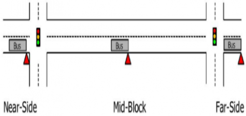
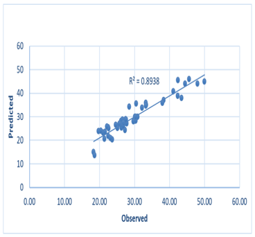
Multiple regression analysis was improved using SPSS and Microsoft excel programs using 43 data points from all routes, to improve two models. The first model has developed a relationship between operating bus speed (Vo) and the other independent variables affecting bus speed with R square 0.89. The second model has predicted the relation between bus operating speed, private vehicle speed, and the number of stops with R square 0.96. Twenty-one data points have been used in validation (testing) for two models. Figure 2 and Figure 3 show plots for predicted versus measured values for operating bus speed for models 1 and 2, respectively.
The summary for the best result for multiple regression models are:
Model 1: correlation between bus operating speed time and other independent variables as shown in Eq. (7).
$\mathrm{V}_{\mathrm{o}}=44+0.56 * \mathrm{~L}-0.62 * \mathrm{~S}-1.2 * \mathrm{I}-0.02 * \mathrm{~V}$ (7)
where,
Vo: Bus operating speed (km/hr).
L: Route length (km).
S: Number of stops.
I: Number of intersections
V: Average traffic volume (vehicle/hr/lane).
Table 4 shows the regression statistics for model 1.
The parameter estimates for operating bus speed; the p-value showed the factors are statistically significant, the negative sign of coefficients explains that the bus operating speed will decrease when the stops, intersections, and traffic volume increased, on the other side the positive sign shows that the operating speed increase as the length of the route increase, as illustrate in Table 5.
Although p-values are provided to assess statistical significance, we recognize the value of including confidence intervals in these estimates. Confidence intervals provide a more accurate understanding of the precision and potential range of the regression coefficients. In future analyses, we aim to include confidence intervals to provide readers with a more complete assessment of the strength and practical relevance of our results.
Model 2: predicting bus operating speed using private vehicle speed at the same route as shown in Eq. (8).
$\mathrm{V_o}=3.76+0.78 \mathrm{V_p}-0.211 \text{S}$ (8)
where,
Vo: Bus operating speed (km/hr).
Vp: Privet vehicle speed (km/hr).
S: Number of bus stops.
Table 6 shows regression statistics for model 2.
Table 7 illustrates the parameter estimates for operating bus speed, P-value showed the factors are statistically significant. Including confidence intervals alongside p-values for the regression coefficients would offer a more precise understanding of the estimates' reliability.
The negative coefficients related with stops, intersections, route length, bus operating speed, and traffic volume provide identified insights with an essential implication for transportation planning:
Stops and Intersections: The unexpected negative relationship between stops, intersections, and shorter bus travel times prompts a reassessment of conventional assumptions.
Route Length and Bus Operating Speed: Negative coefficients for route length and bus operating speed emphasizes the potential gains in travel time efficiency with shorter, more direct routes and ideal bus speeds.
Traffic Volume: The negative coefficient associated with traffic volume challenges assumptions and suggested a counterintuitive relationship between higher traffic density and shorter bus travel times.
In conclusion, these findings advocate for a reevaluation of traditional paradigms in transportation planning. The study underscores the importance of adaptive strategies, grounded in these nuanced insights, to optimize public transportation systems for heightened operational efficiency.
ANOVA Test: Analysis Of Variance (ANOVA), it has been performed at a 95% confidence level to decide if there is a significant relationship between the dependent variable and independent variables. Calculations were made in case there is a committed relationship between the dependent variable and independent variables. Table 8 shows a significant relationship for models 1 and 2.
Our ANOVA results reveal a significant relationship between the variables being studied, but it is crucial to consider the assumptions that underlie this analysis. One key assumption is the normality of residuals. After a closer examination, we observed a slight deviation from normality in the distribution of residuals. Nonetheless, it is worth noting that ANOVA can withstand deviations from normality, especially with larger sample sizes.
Table 4. Regression statistics model 1
|
Paeamater |
Value |
|
R Square |
0.888 |
|
Adjusted R Square |
0.883 |
|
Standard Error |
2.779 |
|
Observations |
43 |
Table 5. Parameter estimates for model 1
|
|
Coefficients |
Standard Error |
t Stat |
p-Value |
|
Intercept |
44.044 |
2.479 |
17.764 |
0.000 |
|
Length |
0.594 |
0.156 |
3.794 |
0.000 |
|
Stops |
-0.628 |
0.110 |
-5.726 |
0.000 |
|
Intersection |
-1.200 |
0.378 |
-3.178 |
0.003 |
|
Volume |
-0.021 |
0.002 |
-8.609 |
0.000 |
Table 6. Regression statistics model 2
|
Paeamater |
Value |
|
R Square |
0.966 |
|
Adjusted R Square |
0.96 |
|
Standard Error |
1.501 |
|
Observations |
43 |
Table 7. Parameter estimates for model 2
|
|
Coefficients |
Standard Error |
t Stat |
p-Value |
|
Intercept |
3.768 |
1.487 |
2.533 |
0.015 |
|
Privet Vehicle Operating Speed (km/hr) |
0.779 |
0.029 |
26.653 |
0.000 |
|
Number of stops |
-0.212 |
0.066 |
-3.193 |
0.003 |
Table 8. Summary results of ANOVA test for models 1 and 2
|
Model 1 |
df |
SS |
MS |
F |
Significance F |
|
Regression |
4 |
2797.126 |
699.281 |
90.487 |
0.000 |
|
Residual |
38 |
332.304 |
7.728 |
|
|
|
Total |
42 |
3129.430 |
|
|
|
|
Model 2 |
df |
SS |
MS |
F |
Significance F |
|
Regression |
2 |
2919.657 |
1459.828 |
648.021 |
0.000 |
|
Residual |
38 |
101.374 |
2.253 |
|
|
|
Total |
42 |
3021.030 |
|
|
|
4.2 Model validation
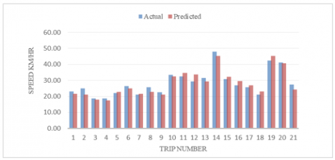
A validation approach must be implemented to check the model reality. In this study, two methods of validation have been applied on different 21 trips selected randomly from four routes.
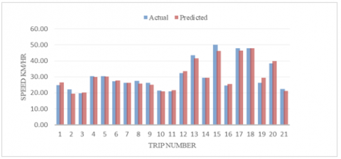
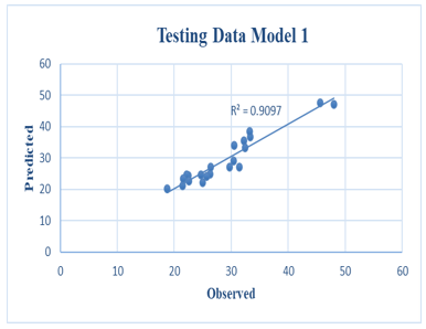
Figures 4 and 5 show a small difference between actual and predicted bus operation speed for models 1 and 2, respectively.
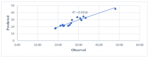
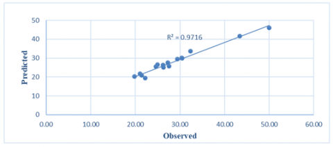
The R2 for validation data has been determined for each model. The result showed a high value of R2 with 0.915 and 0.97 for models 1 and 2 in series, as shown in Figures 6 and 7 respectively.
Also, Thiel's inequality coefficient (U) was employed to validate the model. This parameter provides a measure of how well-estimated values compare to corresponding observed values. The U value varies from 0 to1. The closer the value of U is to zero, the better the forecast method and best fit between observed and predicted values. A value of 1 means the worst forecast and bad fit between observed and predicted values Toledo and Koutsopoulos [20].
$U=\frac{\sqrt{\frac{1}{N} * \sum_{n=1}^N\left(V_{\text {o obs }}-V_{\text {o est }}\right)^2}}{\sqrt{\frac{1}{N} \sum_{n=1}^N\left(V_{\text {o obs }}\right)^2}+\sqrt{\frac{1}{N} \sum_{n=1}^N\left(V_{\text {o est }}\right)^2}}$ (9)
The results of U-coefficient values and average percentage error for two models shown in Table 9 describe a good, predicted model.
As mentioned previously, the U-coefficient value has varied from 0 to 1. The large value of U reflects the model's poor ability to predict accurately by Naghawi et al. [21]. For a good predicting model, the U-coefficient should be less than 0.3. In this study, the U value for both training and testing data records was very small, so the developed model is accurate and efficient.
Figure 4. Actual bus operating speed vs. predicted for model 1
Figure 5. Actual bus operating speed vs. predicted for model 2
Figure 6. Plot of predicted operating bus speed against measured for validation data model 1
Figure 7. Plot of predicted operating bus speed against measured for validation data model 2
Table 9. Thiel's inequality coefficient (U) and average percentage error % result summary
|
|
Model 1 |
Model 2 |
Stage |
|
Thiel's inequality coefficient (U) |
0.04 |
0.02 |
Training |
|
Average percentage error % |
7.9 |
4.3 |
|
|
Thiel's inequality coefficient (U) |
0.04 |
0.03 |
Testing |
|
Average percentage error % |
7.7 |
3.8 |
4.3 Gene Expression Programming (GEP)
We selected Gene Expression Programming (GEP) due to its adaptability, ability to construct features automatically, scalability, interpretability, and resilience. In contrast to alternative approaches, GEP can manage intricate connections, adjust to data traits, scale effectively, generate models that are easy to understand, and mitigate overfitting. These benefits align well with our research objectives.
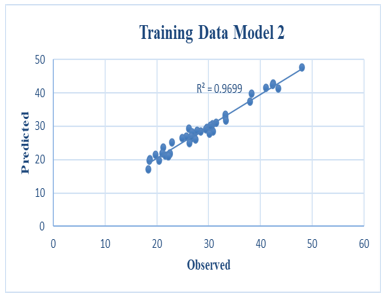
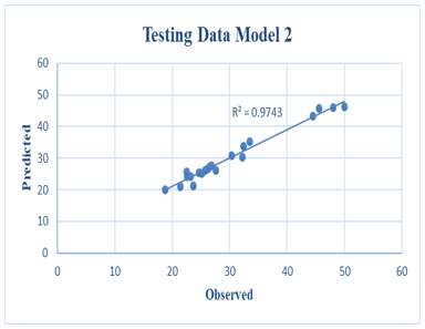
Two models have been predicted using (GeneXpro5.0) software that is based on the Darwinian principle to solve problems. Sixty-four data points were used to predict correlations between operating bus speed and other independent variables for model 1, also for model 2 to predict and operate bus speed depending on private vehicle speed and the number of stops. There are two major stages in the GEP software process: training and validation (testing), (43) 70% of data records were randomly selected from input data, and employed to train the model and learn the relationship between input variables and output variables. In the testing phase, the remaining 21 independent data records which formed 30% of input data were used to test the developed GEP model.
The model development is based on a number of genes that have non-linear behaviors but their combination in a linar form shapes the final structure of the goal model. This GEP model is composed of 30 chromosomes, 3 genes, and 2 genes for model 1 and model 2, respectively. as mentioned previously. The head and intermediate nodes represent mathematical function while the tail nodes represent the independent variables or constant values, in this model the head and tail sizes were 8 and 9, respectively. Table 10 shows Gene Expression parameter estimates for model l and model 2, respectively.
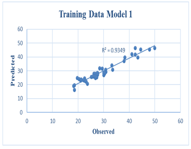
The models have been exhibited in Figures 8 and 9 that show the regression plot for predicted bus operating speed versus measured for training and testing data for models 1 and 2, respectively.
Our research provides valuable insights into the dynamics of bus travel time in our specific urban area. It is important to consider how well our models can be applied to different urban settings and bus systems. While our models provide a basic for understanding the factors influencing travel times, the applicability of our models may vary depending on factors such as infrastructure, population density, traffic patterns, and public transportation policies in different cities or regions. Future research could examine the transferability of the model to different urban environments, perhaps through cross-validation with data from other locations or external validation.
Table 10. Gene Expression Parameter estimates for models 1 and 2
|
Model 1 |
|||||||
|
Independent |
Correl (vs Response) |
Training |
Testing |
Training |
Testing |
Training |
Testing |
|
Stop |
-0.695 |
Average percentage error % |
R-square |
Thiel's Inequality Coefficient (U) |
Stop |
-0.695 |
Average Percentage Error % |
|
Volume |
-0.81 |
6.2 |
7.2 |
0.9349 |
0.9097 |
0.03 |
0.04 |
|
Length |
0.447 |
||||||
|
Intersection |
-0.577 |
||||||
|
Model 2 |
|||||||
|
Independent |
Correl (vs Response) |
Training |
Testing |
Training |
Testing |
Training |
Testing |
|
Stop |
-0.572 |
Average Percentage Error % |
R-Square |
Thiel's Inequality Coefficient (U) |
Average Percentage Error % |
R-square |
Thiel's Inequality Coefficient (U) |
|
Private Vehicle Speed |
0.972 |
3.9 |
4.0 |
0.969932 |
0.97433 |
0.02 |
0.03 |
Figure 8. The regression plot of predicted bus operating speed against measured for testing and training data for gene expression model 1
Figure 9. The regression plot of predicted bus operating speed against measured for testing and training data for gene expression model 2
Because of the congestion problem and to encourage passenger use of public transportations instead of the private vehicle, this study discussed the factors affecting the bus travel time that are operating with mixed traffic for a minibus in Amman and developed two models to predict bus operating speed by using SPSS and Gene Expression Programming (GEP). The model for predicting bus operating speed in mixed traffic lanes in Amman was developed using multiple regression analyses and genetic algorithm techniques with a 95% confidence level. The main factors affecting the bus travel time were the number of bus stops, the number of intersections, traffic volumes, and route length. These factors achieve a highly significant relationship with bus travel time.
The results of model 1 showed: the number of bus stops, signalized intersections, route length, and the average traffic volume are the most effective factors that affect Bus operating speed. Also, the predicted model has a high coefficient determination (R-square) with 0.888 and 0.93 for SPSS and GeneXpro5.0, respectively.
This result showed that the genetics algorithm gave a stronger relationship and more efficient model than multiple regression using SPSS. The results of Model 2 showed: the number of bus stops and the speed of the private vehicle have a strong relationship with the bus operating speed with the coefficient of determination (R-square) with 0.96 and 0.97 for SPSS and GeneXpro5.0, respectively. This result shows that there is no significant difference between the two techniques. Model 2 can help the planning engineers to predict bus operating speed for the new routes by knowing the private vehicle speed and the number of proposed bus stops along the new routes.
The following recommendations are depending on the observation of the transit system should be taken into consideration:
1-The authorities must enforce bus drivers to stop only in their certified locations for boarding and lighting passengers.
2-Greater Amman Municipality (GAM) should improve the public transportation system by studying the possibility of using an exclusive bus lane to attract more passengers and reduce the delay This achieved by collaboration between transport authorities and urban planners is essential. Identifying the main bus routes, conducting feasibility studies, and obtaining public support are important steps. In addition, flexible lane allocation strategies, such as dynamic bus lanes during peak hours, can also be explored to mitigate potential problems.
3-Using the bus with multi-door to reduce the dwelling time.
4-Improve the reliability and serviceability of the transit system.
5-Improve quality control over the bus operators.
6-To improve the transit system in Amman, future research should be taken into consideration and implemented, such as fuel consumption, cost of delay time, maintenance of exclusive lanes, and the effect of weather conditions on bus operating speed.
Studies on the impact of bus travel are crucial for understanding transportation efficiency, accessibility, and urban planning. They can improve efficiency by identifying bottlenecks and inefficiencies in bus routes, improving accessibility by identifying areas with limited access and addressing environmental impact by optimizing routes and infrastructure. Technological advancements like real-time tracking systems and predictive analytics can further refine bus travel times. Future studies should focus on assessing the effects of interventions, exploring the link between travel time variability and passenger contentment, evaluating alternative transportation modes, integrating social equity and environmental sustainability into transportation planning, and exploring the potential of emerging technologies like autonomous vehicles and electrification.
This research can be used for study the effect of bus stops specification and performance on the Bus operating speed and the Impacts of Bus Stops near Signalized Intersections on bus operating speed.
Although our study focuses on a specific geographic area and time period, we recognize the potential impact of changes in local transportation patterns. This realization prompted deep reflection on the generalizability of our findings. We encourage future research to explore the applicability of our results to different urban environments with different traffic dynamics, as this will provide a more comprehensive understanding of the factors influencing bus travel time predictions.
At its core, our methodology seeks to balance specificity and generality, laying the foundations for developments that adapt to different urban landscapes and transport systems.
[1] Tu, T.V., Sano, K., Tan, D.T. (2013). Comparative analysis of bus lane operations in urban roads using microscopic traffic simulation. Asian Transport Studies, 2(3): 269-283. https://doi.org/10.11175/eastsats.2.269
[2] Wei, L., Chong, T. (2002). Theory and practice of bus lane operation in Kunming. DISP-The Planning Review, 38(151): 68-72. https://doi.org/10.1080/02513625.2002.10556825
[3] Figliozzi, M.A., Feng, W.C., Lafferriere, G., Feng, W. (2012). A Study of Headway maintenance for bus routes: Causes and effects of “bus bunching” in extensive and congested service areas. OTREC-RR-12-09.Portland, OR: Transportation Research and Education Center (TREC). https://doi.org/10.15760/trec.107
[4] Mazloumi, E., Currie, G., Rose, G. (2010). Using GPS data to gain insight into public transport travel time variability. Journal of Transportation Engineering, 136(7): 623-631. https://doi.org/10.1061/(ASCE)TE.1943-5436.0000126
[5] Evans, H.K., Skiles, G.W. (1970). Improving public transit through bus preemption of traffic signals. Traffic Quarterly, 24(4).
[6] King, R.D. (1996). Bus Occupant Safety. Transit Cooperative Research Program (TCRP) Synthesis 18. Transportation Research Board, Washington.
[7] Fitzpatrick, K. Nowlin, R.L. (1997). Effects of bus stop design on suburban arterial operations. Transportation Research Record, 1571(1): 31-41. https://doi.org/10.3141/1571-05
[8] Wu, C.S., Murray, A.T. (2005). Optimizing public transit quality and system access: The multiple-route, maximal covering/shortest-path problem. Environment and Planning B: Planning and Design, 32(2): 163-178. https://doi.org/10.1068/b31104
[9] Chen, S.K., Zhou, R., Zhou, Y.F., Mao, B.H. (2013). Computation on bus delay at stops in Beijing through statistical analysis. Mathematical Problems in Engineering, 2013: 745370. https://doi.org/10.1155/2013/745370
[10] Kumar, B.A., Vanajakshi, L., Subramanian, S.C. (2017). Bus travel time prediction using a time-space discretization approach. Transportation Research Part C: Emerging Technologies, 79: 308-332. https://doi.org/10.1016/j.trc.2017.04.002.
[11] Chien, S.I.J., Ding, Y.Q., Wei, C.H. (2002). Dynamic bus arrival time prediction with artificial neural networks. Journal of transportation engineering, 128(5): 429-438. https://doi.org/10.1061/(ASCE)0733-947X(2002)128:5(429)
[12] Chien, S.I.J., Kuchipudi, C.M. (2003). Dynamic travel time prediction with real-time and historic data. Journal of transportation engineering, 129(6): 608-616. https://doi.org/10.1061/(ASCE)0733-947X(2003)129:6(608)
[13] Moridpour, S., Anwar, T., Sadat, M.T., Mazloumi, E. (2015). A genetic algorithm-based support vector machine for bus travel time prediction. In 2015 International Conference on Transportation Information and Safety (ICTIS), Wuhan, China, pp. 264-270. https://doi.org/10.1109/ICTIS.2015.7232119
[14] Farhan, A., Shalaby, A., Sayed, T. (2002) Bus travel time prediction using AVL and APC. In: Applications of Advanced Technologies in Transportation, pp. 616-623. https://doi.org/10.1061/40632(245)78
[15] Qi, W.W., Wang, Y.H., Bie, Y.M., Ren, J. (2021). Prediction model for bus inter-stop travel time considering the impacts of signalized intersections. Transportmetrica A: Transport Science, 17(2): 171-189. https://doi.org/10.1080/23249935.2020.1726525
[16] Yu, B., Wang, H.Z., Shan, W.X., Yao, B.Z. (2017). Prediction of bus travel time using random forests based on near neighbors. Computer-Aided Civil and Infrastructure Engineering, 33(4): 333-350. https://doi.org/10.1111/mice.12315
[17] Bae, S. (1995). Dynamic Estimation of Travel Time on Arterial Roads by Using Automatic Vehicle Location (AVL) Bus as a vehicle Probe. Virginia Polytechnique Institute and State University.
[18] McKnight, C.E., Levinson, H.S., Ozbay, K., Kamga, C., Paaswell, R.E. (2004). Impact of traffic congestion on bus travel time in northern New Jersey. Transportation Research Record, 1884(1): 27-35. https://doi.org/10.3141/1884-04
[19] Vuchic, V.R., Day, F.B., Dirshimer, G.N., Kikuchi, S., Rudinger, D.J. (1978). Transit Operating Manual. Scholarly Commons Collections. https://repository.upenn.edu/handle/20.500.14332/34056.
[20] Toledo, T., Koutsopoulos, H.N. (2004). Statistical validation of traffic simulation models. Transportation Research Record, 1876(1): 142-150. https://doi.org/10.3141/1876-15
[21] Naghawi, H., Jadaan, K., Al-Louzi, R., Hadidi, T. (2018). Analysis of the operational performance of three unconventional arterial intersection designs: Median U-turn, superstreet and single quadrant. International Journal of Urban and Civil Engineering, 12(3): 387-395.