Sheena Mathews*![]() | Tessy Thadathil
| Tessy Thadathil![]()
© 2023 IIETA. This article is published by IIETA and is licensed under the CC BY 4.0 license (http://creativecommons.org/licenses/by/4.0/).
OPEN ACCESS
Transport facilitates growth and interactions within and outside cities. Different countries follow different transport models. Increasing population, rising mobility rate and increasing trip length are responsible for increasing travel demand in India. Intention to participate in activities, demands travel, making it a derived demand. The overall purpose of this study is to examine the impact of socio-demographic factors on the mode of transport for education. The city of Pune in Maharashtra, India is chosen for the study. It is classified into clusters. Seventy-five households are selected from each cluster. For this, socio-economic classification (SEC) is used. The Ordinary Least Square Regression (OLS) model is used for analysis. ANOVA is used to test the effect of income level on the distance travelled for education. In the survey respondents have to give information on employment, education, income, age, sex and travel characteristics. The study found that for education, children generally tend to travel short distances. Children from poorer backgrounds, travel much shorter distances as opposed to children from well-to-do families. They either walk to school or use bicycles. Motorized transport either in the form of school buses or personalized vehicles such as cars or two-wheelers is the norm for children from higher income families. Therefore, their expenditure on travel for education is found to be greater. The paper brings forth issues concerning commuters, especially from a policy perspective. Challenges faced by users of non-motorized facilities such as pedestrian paths, and bicycling paths are brought forth explicitly. The paper looks beyond solutions by institutions which aim to move vehicles rather than people. Broader roads only encourage more use of personalized transport. Instead, differing modes of transport should ensure greater safety to children.
non-motorized transport, per capita expenditure, average distance travelled, ordinary least squares regression, two-wheeler, mixed traffic, personalized transport, walking, cycling
Cities have evolved as a hub where cultural manifestations, trade, employment, social, economic, political expansion and interactions happen. Cities have been centres for different transactions, communications and growth. It is believed that with time more than half of the world’s population will reside in cities. Interactions in places, locations, and spaces are possible due to the availability of different modes of transport. Movement is the crux of one’s existence. The movement has enabled interactions. Alexander's journey and Columbus's voyages created economies and colonies. Transportation has enabled the growth and progress of cities in varying shapes and sizes. Thus, travel is the essence of our existence. Different countries in the world follow various transport models. In the West, the emphasis has been on the use of private cars, whereas in Latin America and Japan, the emphasis has been on public transport. Kenworthy [1] reports that developed countries have a high count of cars per 1000 persons, indicating high car usage. The USA has the highest count of a car-oriented system followed by Australia and European Cities. Due to high dependence on motorized vehicles in cities in America and Australia/New Zealand there is a greater incidence of urban travel and distance covered. This is reflected in terms of high total trips by motorised private modes. Transport is interrelated with the urban form. American, Australian and Western European cities are less densely populated, consequently auto dominance is reflected. Asian cities have the least car dependence. Car ownership in Asian cities is less than half of Europe and Australia. In spite of that Asian cities are denser and these cities require "space-efficient and low-impact modes of transport" like public transit (E_Public_mode) and non-motorised mode of transport (E_NMT_mode). Non-motorised trips are high in Asia, Europe and Latin America. USA and ANZ have a very low percentage of non-motorised trips. Barter [2] reports that in the case of two-wheeler ownership and use, Asian cities have a very high usage of two-wheeler. The count is high due to congested traffic environments in the absence of competitive, convenient, and comfortable public transport systems. The two-wheeler has replaced the bicycle in most Asian cities. The popularity of the two-wheeler over the cycle is because it involves lesser physical burden, less travel time and easy manoeuvrability. Despite its benefits, the two-wheeler has been objected to in some countries since it disrupts traffic, occupies too much road space, and dilutes the market for public transport. The Asian cities have less than half of the road provision of Europe and far lower than Australia and the USA. The length of road per person is less in developing countries i.e., as low as 0.6 metres per person. It is due to these reasons that roads fill up despite low levels of vehicle ownership. The time spent commuting has remained relatively constant in the range of about 90 minutes per day. This is known as Marchetti's constant in the name of the physicist who established the relation. Because of its high level of motorization, the United States has the lowest average commuting time in the world, around 25 minutes in 1990 (one direction) with a global average in the range of 30 minutes. The cities in Western Europe and Japan are relatively more compact and the commuters depend more on walkability and public transport. As a result, their commuting times are longer. There is, thus, an inverse relationship between the level of public transit use and commuting time as passengers tend to spend more time waiting and transferring within the transit system. Rodrigue [3] illustrates that the last decade has shown growing commuting times, mainly due to increasing congestion levels in metropolitan areas. India has experienced a tremendous increase in the total number of registered motor vehicles. Travel demand is increasing significantly over the years. The increasing population, rising mobility rate and increasing trip length are responsible for increasing travel demand in India. The urban population has increased at a tremendous pace. This means there is greater demand for mobility in cities. Mobility rate is the average number of trips per person per day. This rate has increased. According to EMBARQ [4], the average number of trips per person per day for Mumbai, Kolkata, Chennai, Hyderabad, Bangalore, Ahmedabad, and Pune are 1.26, 1.26, 1.22, 1.05, 1.20, 1.57, and 1.48 respectively. Another factor contributing to the rise in travel demand is the increase in trip length due to an increase in the physical expansion of the city. Currently, it is estimated that the average trip length of four mega cities varies from 12.7 to 13.5 km. Mode share is also called modal split. It indicates the mode of travel used by a traveller. The modal share in the selected 30 cities shows that cities with a higher percentage of public transport have lower personalised transport. According to Ministry of Urban Development [5], the metros (Delhi, Chennai, Kolkata, Mumbai) have a high share of public transport. Delhi and Kolkata which have a high share of public transport have a lower share of the two-wheeler. Cities with poor or no public transport are Agra, Patna, Gangtok, Bikaner, Raipur, Amritsar, Varanasi and Surat. Cities like Gangtok, Bikaner, and Raipur have a greater share of walking and cycling. Tourist cities i.e. Agra, Amritsar, Patna, Varanasi and Surat have a greater share in Intermediate Public Transport (IPT). Walk trips are greater in smaller cities and cycle trips are low in hilly cities.
Travel is a derived demand since it helps to undertake activities. The activities undertaken would require either frequent travel or occasional travel. In the case of education and/or work trips, it involves frequent movement. The choice of mode of transport involved assumes that people make rational choices from the alternatives available, to maximize satisfaction. Cities in India have mixed land use and mixed traffic. Bicycles, pedestrians and motorised modes are present in significant numbers on urban streets. The co-existence of nonmotorized transport and motorized transport has its challenges in terms of speed, safety, the flow of vehicles etc.
The purpose of the study is to examine the impact of socio-demographic factors on the mode of transport for education and to determine the relationship between the per capita expenditure incurred by the households for education. The choice of where to stay in the city is a tough one. People who tend to stay in the city are troubled by increasing air and noise pollution, congestion, expensive housing and traffic-related hazards. The growing size of population and increasing city size has pushed certain segments of people to the periphery, to face largely non-existent public services, long commuting to the city, increased reliance on motorized transport, and less feasibility of walking and cycling.
Pune is the eighth largest city in India and the second largest city in Maharashtra after Mumbai. Pune is known as the "Oxford of India" which reflects the importance of Education in the city. In India school education is provided by Government and private entities. There are different boards which provide school education. The state board is specific to the state that the child belongs. The Central Board of Secondary Education (CBSE) and Indian Certificate of Secondary Education (ICSE) Boards are all across the country. In this case, the same syllabus is taught to children across schools. The school fees vary depending on the type of school the children are in. India has a 10+2 pattern for school education. This study is restricted to children up to 10th grade. Education requires mandatory travel. After the admission is given, the only choice the student can make is to choose the mode of travel. The choice of mode is majorly determined by the earnings of the household. The purpose of the study is to examine the per capita expenditure incurred by households for education. Also, the choice of the mode of transport for education is examined. For the study, Pune city was classified into six clusters. From each of the clusters, seventy-five households were selected. To select households from each cluster, socio-economic classification (SEC) is used. SEC is used by the Market Research Society of India (MRSI) to classify households based on two variables: the education of the chief earner and occupation.
Travel demand management involves various policy measures and strategies to reduce travel demand and improve the urban transport system. The push effects are congestion pricing, speed restrictions, car-free zones. Also push measures are aimed at attracting people towards public transport, usually by providing quality public transport service, subsidies and alternative means. Pull measures, are designed to tackle private transport, mainly car usage by imposing higher tolls, higher parking etc. Pull effects are a preference for public transport, pedestrian facilities, and cycle networks. Walking connects many trips, like home to bus, shopping, parking lots, etc. The choice of mode is limited by time and budget. Individuals have a threshold of time beyond which travelling is not perceived as right. According to Burbidge and Goulias [6] often the choice of travel by the walk mode is done keeping these constraints in mind. Litman [7] states that walking provides a variety of benefits, including accessibility, transportation cost savings, public health, more efficient land use, and community liveability. The inclusion of non-motorized trips can translate into favourable public health consequences. Ibrahim [8] explains that car is favoured for its safety from crime, flexibility, speed, directness of travel, weather protection, the privacy of travel and minimal waiting time in travel. De Jong and van de Riet [9] explain that in developed nations, an increase in income leads to a shift of modes, from non-motorized travel to cars. In developing nations, the increase in income leads to a shift from non-motorized to scooters and motorcycles and then to cars. There is an income threshold at which vehicle (specifically auto) ownership is possible. Gakenheimer and Zegras [10] elucidates that personal car ownership versus income follows an S-curve (logistic curve). In the case of developing countries, a vast majority of the population is still at income levels below the rising portion of the S-curve, which means that higher income leads to higher car ownership. But in the case of developed countries, initially, with an increase in income, there is an increase in car ownership, but further increases in income see an attenuation in vehicle ownership.
Travel would be determined not only by the activity the person wants to undertake, but also determined by other factors like income, place of stay, transport options, prices etc. Several studies have examined the relationship between travel behaviour and demographic variables such as gender, age, income, employment status, educational status, household composition etc. The study of Hanson and Hanson [11] gave a comparison between travel to work by men and women indicating that men travel to activity sites that are further away from home than women. The study of Astrop et al. [12] examined factors that would influence travel demand patterns of households from lower income. Income is an important factor in deciding the mode of travel to be used. Women who are earning tend to use personalized transport. The women used either two -wheelers or mopeds to reach their workplaces. In some instances, women were not even allowed to use bicycles for transportation. There was greater reliance on public transport and cycling to meet the mobility requirements.
Urban Form affects the amount of travel. Soltani and Primerano [13] undertook a case study of Adelaide in South Australia where households were randomly selected and attempted an empirical model that incorporates built environment features into vehicle ownership models. It was observed that the further the family lived away from the Central Business District (CBD), the more the likelihood to own two or more vehicles. The study also looked into how auto ownership is affected by socio-economic factors such as household size, household type, household income, and dwelling structures and urban structure characteristics such as density, land use mix, distance to workplace and design features. In the Indian context, Srinivasan and Rogers [14] show the impact of urban form on the travel behaviour of households of two areas in the urban area of Chennai was studied. One area is located in the centre of the city (Srinivasapuram) and the other at the periphery (Kannagi Nagar). Two significant variables, accessibility to transport modes and the location of employment opportunities, were considered. It was found that there was a difference in the travel behaviour of households due to the location of employment opportunities in the centre of the city. People staying in the centre of the city relied more on walking and cycling to reach the workplaces since these were located closer to their homes. Location affects different aspects of travel behaviour i.e., time spent, cost, frequency and mode choice for the trip. Though walking and cycling to school seem appropriate from a health standpoint. Nelson et al. [15] explain that it may also be due to the financial limitations of parents. Schlossberg et al. [16] pronounce that there is an impact of urban form and distance on travel mode for educational purposes. But urban form is not the only factor which would determine the mode of transport for education. Moreno and Miralles-Guasch [17] explain that bicycles as a mode is used when it's difficult to walk, and access to public transport is not available. Duze [18] explains that travelling for education is stressful for students and parents. The distance travelled can be tiring for students. Despite the use of the car, the distance travelled affects children. Sidharthan et al. [19] show how decisions regarding the mode of transportation for children are affected by spatial interactions. Zhang et al. [20] explain that the use of cars for commuting tends to be higher when the distance between school and home is greater.
The study looks into the distance covered for access for education. The study also looks into the trips undertaken by boys and girls for education i.e. mean distance travelled (in km) and the modal choice. In the study students are those who are undergoing education and are below 20 years. A matrix made on the basis of education and age showed that most students were below 20 years. The study develops a model for education with the household as a unit of measurement. The total student population was 587702 [21]. The sample size was 579 which is adequate to detect the prevalence of distance covered for access to education, with a confidence level of 95%. Of which 304 were male students and 275 were female students. The study looks into the number of trips made for education i.e. daily or more during a week. The study also looks into the trips undertaken by boys and girls for education i.e. mean distance travelled (in km) and the modal choice. ANOVA is used to test the effect of the income level of households, on the distance travelled for educational purposes. School busses, private busses, public transport personalized transport (two-wheeler or car), autorickshaws, cycles and walking are the range of modes of transport used by the children to reach their school.
Hypotheses
H1: There is a significant difference between the mean distance travelled by students for each four income levels.
Ho: There is no relation between distance travelled by students for education and their household income.
The objective of the education model is to determine the relationship between the per capita expenditure incurred by the households for the education of students. The Ordinary Least Square Regression (OLS) model is used for this purpose.
Per Capita Expenditure = Per Capita Income + Average Distance Travelled + Proportion of Students + Mode of Transport (Non-Motorised Transport or Private or Public transport).
Per Capita Expenditure on travelling for education is the dependent variable and Per Capita Income, Average Distance Travelled, Proportion of students, and Mode of Transport (NMT, Private and Public) are independent variables. Mode of transport is a categorical variable having three categories. Non-Motorized Transport (NMT) refers to walking and cycling. Private refers to personalized transport such as a two-wheeler or car. Public refers to buses i.e., public transport, school buses and van. Thus, there is a need to create two dummy variables such as E_NMT_mode and E_Private_mode and Public mode. Dummy variables for a mode of transport can be created as follows:
$\begin{aligned} & \text {E_NMT_Mode } = \begin{cases}1, & \text { if there are NMT users in household } \\ 0, & \text { otherwise }\end{cases} \end{aligned}$ (1)
$\begin{aligned} & \text { E_Private_Mode } = \begin{cases}1, & \text { if there are private users in household } \\ 0, & \text { otherwise }\end{cases} \end{aligned}$ (2)
If both are zero then the mode of transport is a public mode. The ordinary Least Squares Method which is defined above is used to estimate regression coefficients.
The study analysed the distance travelled by a student to the educational institute from home. It is observed that 77% of student respondents travelled less than 5 km for educational purposes. In the case of distances less than 1 km, female students (16.41%) travelled more than male students (14%). Only 11 students out of 579 travelled more than 15km for education, of which 9 were boys. This shows that parents are fine with a boy child travelling a longer distance than a girl child travelling. The analysis is with respect to households. Table 1 examines distances travelled for the purpose of education under different income segments
Results from ANOVA Table 2 and data from Table 1 show that the null hypothesis is rejected at 1 per cent level of significance. There is a significant difference between the mean distances travelled by students in each of the income segments. This verifies the fact that students from lower-income households travel shorter distances for educational purposes.
Table 1. Descriptive statistics about distance for education under different income segments
|
Income Slab |
N |
Mean |
Std. Deviation |
Std. Error |
95% Confidence Interval for Mean |
Minimum |
Maximum |
|
|
Lower Bound |
Upper Bound |
|||||||
|
<₹. 16,000 |
104 |
3.1827 |
4.88661 |
.47917 |
2.2324 |
4.1330 |
.00 |
26.00 |
|
₹. 16,000 - ₹. 30,000 |
71 |
4.6761 |
5.54147 |
.65765 |
3.3644 |
5.9877 |
.00 |
25.00 |
|
₹. 30,000 - ₹. 62,000 |
75 |
8.3333 |
10.73808 |
1.23993 |
5.8627 |
10.8039 |
.00 |
79.00 |
|
>₹. 62,000 |
65 |
12.1077 |
13.95766 |
1.73123 |
8.6492 |
15.5662 |
.00 |
102.00 |
|
|
315 |
6.5873 |
9.65724 |
.54412 |
5.5167 |
7.6579 |
.00 |
102.00 |
Table 2. ANOVA test for distance in km for education
|
Sum of Squares |
df |
Mean Square |
F |
Sig. |
|
|
Between Groups |
3674.358 |
3 |
1224.786 |
14.873 |
.000 |
|
Within Groups |
25609.991 |
311 |
82.347 |
||
|
Total |
29284.349 |
314 |
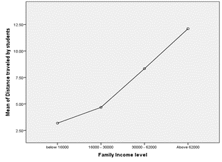
Figure 1. Distance travelled by students (in km)
Figure 1 shows that the mean distance travelled for education, increases with the increase in income level.
4.1 Model of travel demand for education
The coefficient of determination Table 3 shows that 70% of the dependent variable (per capita expenditure) is explained by the predictors (E_Private_mode, Prop_student, Average_Ekm_bs, PCIncome, E_NMT_mode.
Table 4 shows the significance value of .000 which indicates that the regression model is statistically significant
Table 5 shows that the average distance travelled for education, per capita income, NMT mode and private mode used to reach a place of education is statistically significant at 1 per cent level of significance.
Table 3. Model summary of travel demand for education
|
Model |
R |
R Square |
Adjusted R Square |
Std. Error of the Estimate |
|
1 |
.840a |
.705 |
.700 |
12.09 |
a. Predictors: (Constant), E_Private_mode, Prop_student, Average_Ekm, PCIncome, E_NMT_mode
b. Dependent variable: Per capita expenditure.
Table 4. ANOVAa test of travel demand for education
|
Model |
Sum of Squares |
df |
Mean Square |
F |
Sig. |
|
|
1 |
Regression |
107858.835 |
5 |
21571.767 |
147.622 |
.000b |
|
Residual |
45153.827 |
309 |
146.129 |
|||
|
Total |
153012.662 |
314 |
||||
a. Dependent Variable: E_PCexp
b. Predictors: (Constant), E_Private_mode, Prop_student, Average_Ekm, PCIncome, E_NMT_mode
Table 5. Coefficientsa of travel demand for education
|
Model |
Unstandardized Coefficients |
Standardized Coefficients |
t |
Sig. |
||
|
B |
Std. Error |
Beta |
||||
|
1 |
(Constant) |
7.694 |
2.678 |
2.873 |
.004 |
|
|
Average_Ekm |
.767 |
.094 |
.305 |
8.148 |
.000 |
|
|
PCIncome |
.0003 |
.0001 |
.177 |
5.008 |
.000 |
|
|
Prop_student |
5.572 |
5.294 |
.034 |
1.053 |
.293 |
|
|
E_NMT_mode |
-11.899 |
1.943 |
-.268 |
-6.123 |
.000 |
|
|
E_Private_mode |
16.975 |
1.692 |
.380 |
10.035 |
.000 |
|
a. Dependent Variable: E_PCexp
4.2 Discussion
In this study travel demand has been examined with households as a unit of measurement. It was rather difficult to gather the relevant data from households but nonetheless it was an enriching experience. It involved the formidable task of collecting information from urban respondents who were invariably tied up with household chores, work etc. The respondents from the lower income groups were keen to know the benefits they would derive by sharing information with the researchers.
The study was carried out to examine the relationship between per capital expenditure on travel incurred by households for education as also to build a model to understand the impact of socio demographic factors on the mode of transport for education
The analysis is with respect to households. Table 1 clearly brings out the fact that out of the 315 households, those households for which the mean travel for education was 3.1827 fell in the income bracket of less than Rs16000 while those whose mean distance travelled stood at 12.1077 fell in the income bracket of greater than Rs 62000. Thus, it proves that there is a positive relationship between the distance travelled by students for education and their income. Therefore, the H1 hypothesis is accepted showing that there is a significant difference between the mean distance travelled by students from households in each of the income levels
With the increase in household income, families tend to keep aside a higher budget for travel. They are open to sending their children by personalized mode of transport. Families prefer that their children travel comfortably. Also, personalized mode would mean that they can choose a convenient time for leaving home to reach school. Personalized transport would also mean greater safety. Safety could be in terms of travel as also safety from getting infections through public modes of transport. Many a child from well-to-do families travel long distances for education.
The study found that for education children generally tend to travel short distances. Children from low income groups in particular tend to travel shorter distances. The primary reason for this is that they save on travel expenses and sometimes that is the only option given a shoestring budget. These shorter distances are covered either by cycling or walking. This saving on travel expense can therefore be diverted to other family requirements. The boy child is given preference to use a bicycle for going to school.
Besides personalized transport like a two-wheeler or a car, walking and cycling, the other modes to reach school are school buses, private buses, public transport, autorickshaws etc. But there are several challenges faced by children using these different modes. For example, children who walk to school find it difficult to cross roads at intersections. Footpaths are heavily encroached in many cities and the quality of footpaths is not always good. This is another problem faced by children walking to school. Those children who resort to public transport like the bus, face challenges of fares being too high, bus stops being far from place of residence, buses not stopping at bus stops, frequency of buses being poor, buses not going directly to intended destination, difficulty in exiting crowded buses, unhygienic buses, lack of courtesy of bus staff, danger of harassment by co travelers, theft, inadequate information on routes etc.
The regression model shows that 70% of the dependent variable i.e., E_PCexp (per capita expenditure on travel for education) is explained by the predictors i.e., E_Private_Mode, Prop_student, Average_Ekm, PCIncome, E_NMT_mode.
If this study had collected data on the basis of travel diaries instead of questionnaire-based surveys it would have thrown up even more detailed observations.
Children tend to travel for education. The study found that for education children generally tend to travel short distances. Children from poorer backgrounds travel much shorter distances and would be either walking to school or would be using bicycles. The boy child is given preference to use a bicycle for going to school. Children from well-to-do families travel long distances for education. The use of motorized transport either in the form of school buses or personalized vehicles such as cars or two-wheeler is used. The expenditure on travel for education purposes is greater at higher income levels. The higher income category sees longer distance travelled for education and greater expenditure incurred for the purpose. Even though Cycling and walking are preferred modes of transport by children. The city is challenged by the fact that footpaths either do not exist or are taken over by street vendors. Also, the large number of personalized transport makes cycling and walking an unsafe and unhealthy option for children
From a policy perspective, the researchers feel that the study has been able to bring forth several issues especially concerning student commuters. More specifically, the challenges faced by users of non-motorized facilities such as pedestrian paths, and bicycling paths are brought forth explicitly. Very often, the solutions provided are in terms of measures which have the objective of moving vehicles rather than people. Such an approach affects a significant part of the population which depends on the walk mode, especially in the traditional but core areas of the city. Equally important is the consideration that the mode of transport that is ultimately used, results in benefits, such as business opportunities, investments, etc. but also externalities by way of social costs such as pollution, congestion etc. The challenge lies in bringing about a change in the behaviour which is determined by several factors. A separate study for the same would be extremely useful. Changing individual behaviour is difficult. This is a challenge for the society and needs to be studied further in depth.
[1] Kenworthy, J. (2011). An international comparative perspective on fast-rising motorization and automobile dependence. In Gakenheimer, R and Dimitriou, H. T. Editor (Ed). Urban Transport in the Developing World: A Handbook of Policy and Practice, pp. 71-112, Edward Elgar Publishing Inc, Massachusetts, USA.
[2] Barter, P.A. (1999). An international comparative perspective on urban transport and urban form in pacific Asia: The challenge of rapid motorisation in dense cities. Ph.D thesis, Murdoch University.
[3] Rodrigue, J.P. (2013). The Geography of Transport System. New York, Routledge.
[4] EMBARQ. (2007). India Transport Indicators – Retrieved from https://environmentaldocuments.com/embarq/India-Integrated-Transport-Indicators-EMBARQ.pdf, accessed on Jun. 18, 2022.
[5] Ministry of Urban Development. (2008). Traffic & transportation policies and strategies in urban areas in India, New Delhi.
[6] Burbidge, S.K., Goulias, K.G. (2008). Active travel behavior. In CD ROM Proceedings of the 88th Annual Transportation Research Board Meeting, January 11-15.
[7] Litman, T.A. (2003). Economic value of walkability. Transportation Research Record, 1828(1): 3-11. https://doi.org/10.3141/1828-01
[8] Ibrahim, M.F. (2003). Car ownership and attitudes towards transport modes for shopping purposes in Singapore. Transportation, 30: 435-457. https://doi.org/10.1023/A:1024701011162
[9] de Jong, G.C., van de Riet, O. (2008). The driving factors of passenger transport. European Journal of Transport and Infrastructure Research, 8(3). https://doi.org/10.18757/ejtir.2008.8.3.3348
[10] Gakenheimer, R., Zegras, C. (2004). Drivers of travel demand in cities of the developing world. In Mobility 2030: Meeting the Challenges to Sustainability, pp. 155-170.
[11] Hanson, S., Hanson, P. (1981). The travel-activity patterns of urban residents: Dimensions and relationships to sociodemographic characteristics. Economic Geography, 57(4): 332-347.
[12] Astrop, A., Palmer, C., Maunder, D., Babu, D.M. (1996). The urban travel behaviour and constraints of low income households and females in Pune, India. In Second National Conference on Women’s Travel Issues, Baltimore, pp. 23-26.
[13] Soltani, A., Primerano, F. (2005). The travel effects of community design. Doctoral dissertation, NSW Transport and Population Data Centre.
[14] Srinivasan, S., Rogers, P. (2002). Travel behaviour of low income residents: Studying two contrasting locations in the city of Chennai,India. In Transport Research Board 2003 Annual Meeting.
[15] Nelson, N.M., Foley, E., O'gorman, D.J., Moyna, N.M., Woods, C.B. (2008). Active commuting to school: How far is too far? International Journal of Behavioral Nutrition and Physical Activity, 5(1): 1-9. https://doi.org/10.1186/1479-5868-5-1
[16] Schlossberg, M., Greene, J., Phillips, P.P., Johnson, B., Parker, B. (2006). School trips: Effects of urban form and distance on travel mode. Journal of the American Planning Association, 72(3): 337-346. https://doi.org/10.1080/01944360608976755
[17] Moreno, C., Miralles-Guasch, C. (2016). The bicycle as a real feeder to the TransMilenio system in Bogota and Soacha. International Journal of Transport Development and Integration, 1(1): 92-102. https://doi.org/10.2495/TDI-V1-N1-92-102
[18] Duze, C.O. (2010). Average distance travelled to school by primary and secondary school students in Nigeria and its effect on attendance. African Research Review, 4(4). https://doi.org/10.4314/afrrev.v4i4.69236
[19] Sidharthan, R., Bhat, C.R., Pendyala, R.M., Goulias, K.G. (2011). Model for children's school travel mode choice: Accounting for effects of spatial and social interaction. Transportation Research Record, 2213(1): 78-86. https://doi.org/10.3141/2213-11
[20] Zhang, R., Yao, E., Liu, Z. (2017). School travel mode choice in Beijing, China. Journal of Transport Geography, 62: 98-110. https://doi.org/10.1016/j.jtrangeo.2017.06.001
[21] PMC Open Data Source School Enrollment Data. http://opendata.pmc.gov.in/Citizen/CitizenDatasets/Index?categoryId=13, accessed on Mar. 18, 2023.