Mariem Jarjar![]() | Hamid El Bourakkadi
| Hamid El Bourakkadi![]() | Abdellah Abid
| Abdellah Abid![]() | Hassan Tabti
| Hassan Tabti![]() | Abdellatif Jarjar*
| Abdellatif Jarjar*![]() | Abdelhamid Benazzi
| Abdelhamid Benazzi![]()
© 2025 The authors. This article is published by IIETA and is licensed under the CC BY 4.0 license (http://creativecommons.org/licenses/by/4.0/).
OPEN ACCESS
Classical Hill polyalphabetic encryption typically uses a small invertible square matrix. Due to its nature as a linear cipher, this approach remains highly vulnerable to frequency and statistical attacks. To overcome such a limitation, we propose in this study a new extension of this technique, using a non-square pseudorandom cipher matrix that significantly increases the time complexity of brute-force attacks. After creating two replacement tables of arbitrary sizes from the most widely used chaotic maps in cryptography, produced by randomly selecting a set of linear congruence generators (LCGs) from a pseudorandom table, we will subject these generators to bijective affine functions in order to introduce noise into the placement of the generated values. This new technique, which consists of the association of two improved norms, begins by segmenting the original image vector by pseudorandom transformations into three-pixel sub-blocks. Then, three additional random pixels were added to form a six-component sub vector that will undergo random local permutation, and then an encryption process is applied using a non-square matrix. The good results obtained from randomly selected images in several databases demonstrated the consistency of the procedure and ensured the robustness of our system.
chaotic map, improved Vigenere cipher, retyped Hill, diffusion function, encryption circuit
Multiple domains, including the military, e-government, traffic inspection, climate forecasting, and natural disaster monitoring, generate an enormous quantity of visual data. The security of multimedia assets, particularly images [1-3], has become a growing concern for both academic researchers and industry professionals. The increasing interconnectedness of our world and the crucial role of the Internet in data transfer have underscored the vulnerability of networks. The inherently open nature of information-sharing techniques creates opportunities for security breaches, allowing malicious actors to intercept and access private data. Consequently, encryption has gained significant importance and is now the only known safeguard against such malevolent attacks.
The quick advancement of mathematical chaos theory offers scientists opportunities to further improve some traditional encryption schemes. Given the significant focus on security, numerous image encryption techniques have overwhelmed the digital landscape, primarily leveraging number theory and chaos [4, 5]. Some are trying to refresh their approaches by optimizing classical methods, including the Hill [6, 7], Cesar, Vigenere [8, 9], Feistel [10], and other relevant techniques such as DNA-based [11] and RNA-based [12, 13].
The problem is that the procedure used in the conventional Vigenere system is vulnerable to frequency and statistical attacks [14, 15] due to the magnitude of the private key recognition problem. Also, the ability to know the substitution matrix offers a chance to expose the conventional methodology to brute force attempts. Furthermore, the conventional Hill approach is open to brute-force attacks since it relies on an invertible square matrix. likewise, all conventional systems, particularly the traditional Hill approach, are vulnerable to differential attacks when no diffusion function and no potential for chaining are applied. Conversely, dictionary and statistical assaults can be more easily implemented with the help of tiny block ciphers. This paper's contribution is twofold: Firstly, it generates massive substitution tables of randomly computed.
To resolve these problems, we developed large substitution tables, which emerge from a coupling of linearly congruent generators of bijective affine operations, to safeguard our novel method against existing assaults. In addition, we will configure the Hill method for tweaking by adopting a non-square encryption matrix.
The remainder of the text is organized into several sections. One section details our approach to elucidating the nuances of the encryption and decryption procedures. Another section presents the experimental results, including statistical and differential metrics. A subsequent section compares our technique with other similar methodologies and studies. Additionally, there is a discussion section that critically examines our findings. Furthermore, a section is dedicated to outlining the advantages and limitations of our method. Finally, the concluding section summarizes the results and provides recommendations for future research.
The three most widely used chaotic maps in the field of cryptography are utilized in this novel approach, which maintains strong resistance against brute force attacks due to their large key size and high sensitivity to initial parameters. Additionally, this novel cryptosystem accepts six pixels as input via a non-square encryption lattice and returns three Pseudo-Random pixels for the encrypted image reconstruction. The axes listed below serve as instruments for explaining this novel algorithm:
2.1 Chaotic sequences selection
Because of their extraordinary sensitivity to initial conditions and easy configuration, our algorithm suggested using the three most researched maps in cryptographic schemes [16, 17]: the logistic, skew tent, and A.J. maps, as illustrated in Figure 1.
Figure 1. Chaotic map selected
2.1.1 The logistics maps
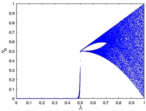
The map un [4], defined as a sensitive recursive formula of a simple second-degree polynomial by Eq. (1), generates real sequences. The bifurcation diagram illustrating the chaotic aspect of the logistics map is given in Figure 2.
$\left\{\begin{array}{l}u_0 \in[0.5 ; 1], \mu \in[3.75 ; 4] \\ u_{n+1}=\mu u_n\left(1-u_n\right)\end{array}\right.$ (1)
Figure 2. Bifurcation diagram of the logistics map
Values for the quantitative assessment of chaotic performance are represented by the Lyapunov exponent. Stated otherwise, the presence of a positive value for the Lyapunov exponent, depicted in Figure 3, indicates that the nonlinear map is sensitive to initial conditions, demonstrates improved chaotic behaviors with respect to the unpredictability characteristic, and also represents the best chaotic performances. From a mathematical perspective, the Lyapunov exponent Eq. (2), looks like this:
$\lambda=\frac{1}{n} \sum_{i=0}^n \operatorname{Ln}\left(\left|f^{\prime}\left(u_i\right)\right|\right)$ (2)
Figure 3. Lyapunov of the logistic map
2.1.2 The skew tent map
The skew tent map (SKTM) (Vn) [18-20] will be redefined as the Eq. (3).
$\left\{\begin{array}{c}\mathrm{v}_0 \in[0 ; 1], \mathrm{p} \in[0.5 ; 1] \\ \mathrm{v}_{\mathrm{n}+1}=\left\{\begin{array}{c}(\mathrm{p})^{-1} \mathrm{v}_{\mathrm{n}}, \text { if } 0<\mathrm{v}_{\mathrm{n}}<\mathrm{p} \\ (1-\mathrm{p})^{-1} \left(1-\mathrm{v}_{\mathrm{n}}\right), \text { if } \mathrm{p}<\mathrm{v}_{\mathrm{n}}<1\end{array}\right.\end{array}\right.$ (3)
This card possesses a highly significant chaotic component for a color image encryption system, as seen by the bifurcation diagram in Figure 4.
Figure 4. Bifurcation diagram of the SKTM
2.1.3 The A.J. map
The A.J. map formula of this map [21, 22] given in Eq. (4), has a great sensitivity to beginning circumstances, chaotic behavior, and ease of implementation are the main reasons it was chosen; its Lyapunov exponent is on the order of $(p * \log (2)>\log (2)$ with $p>1)$.
$\left\{\begin{array}{c}\mathrm{w}_0 \in[1 /(1+p) ; p /(1+p)], \mathrm{p} \in[1.65 ; \varphi] \\ \mathrm{f}\left(\mathrm{w}_{\mathrm{n}}\right)=\mathrm{w}_{\mathrm{n}+1}\left\{\begin{array}{c}\mathrm{p}^2 \mathrm{w}_{\mathrm{n}}, \text { if } 0 \leq \mathrm{w}_{\mathrm{n}} \leq(1+\mathrm{p})^{-1} \\ \mathrm{p}-p \mathrm{w}_{\mathrm{n}}, \text { if } (1+\mathrm{p})^{-1} \leq \mathrm{w}_{\mathrm{n}} \leq 1\end{array}\right.\end{array}\right.$ (4)
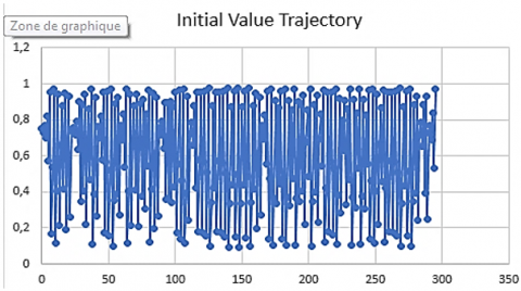
The integration of three chaotic maps in a hybrid approach enables the derivation of all critical parameters required to optimize the efficiency and effectiveness of our innovative architecture. In Figure 5, the chaotic trajectory for an initial value of 0.75 is shown.
(a) Trajectory of the initial value 0.75
(b) Initial conditions sensitivity
Figure 5. Trajectory of the initial value 0.75 and initial conditions sensitivity
These chaotic maps were chosen for our cryptosystem for the following reasons:
Sensitivity to initial conditions.
Random appearance.
Ease of implementation.
2.1.4 Compare the three chaotic maps
Despite the reliability of the three chaotic maps, there are minimal differences between them, as summarized in Table 1. We quote:
Table 1. Mapping function comparison
|
Criteria |
Logistic Map |
PWLCM |
Skew Tent |
|
Complexity |
Quadratic (more complex) |
Piecewise linear (simple) |
Piecewise linear |
|
Uniformity |
Possible bias for some r |
Very uniform distribution |
Good uniformity |
|
Security |
Vulnerability to weak parameters |
Resists short-cycle attacks |
parameters sensitive |
Chaotic Card Advantages.
Low Computational Cost: Ideal for embedded devices.
Large Key Space: Depends on initial condition and control parameters, ensuring high security.
Adaptability: Can be integrated with other systems, such as hybrid chaos or quantum encryption.
Limitations.
Vulnerability to statistical analysis attacks: If poorly implemented, it may require post-processing to enhance security.
Risk of short cycles: Improper selection of control parameters can lead to short periodic sequences.
The combination of these three chaotic maps will be used to generate all the parameters necessary for the proper functioning and operation of our new technology.
2.2 Building encryption tools
This first phase acts at the pixel level by implementing an improved Vigenère technique that uses two large S-Boxes. For the smooth running of this part, several parameters will be developed.
(WC) of size (3 nm;5) confusion/diffusion table.
(WB) of size (3 nm;5) confusion/diffusion binary table.
(WS1); (WS2) two substitution tables of size (t 256), with (t) an integer calculated from the Pseudo-Random vectors and under the control of the binary decision vector.
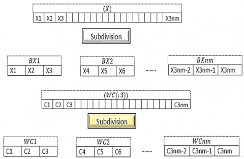
The construction of all these parameters is illustrated in Figure 6.
Figure 6. Encryption tools generation
2.2.1 (WC) Confusion/diffusion table design
The (WC) table of size (3 nm;5) with coefficients in (G256) is used to facilitate communication and diffusion among the original image pixels. It has been spoken regarded as an encryption subkey. The construction of this table is described by Algorithm 1.
|
Algorithm 1: (WC) Confusion/Diffusion Table Design |
|
$\begin{aligned} & \text { 1. For } j=1 \text { to } 3 \mathrm{~nm} \\ & \text { 2. } W C(j ; 1)=\operatorname{Int}\left(|v(j)+u(j)| * 10^{10}\right) \% 252+3 \\ & \text { 3. } W C(j ; 2)=\operatorname{Int}\left((u(j)-v(j)) * 10^{12}\right) \% 250+4 \\ & \text { 4. } W C(j ; 3)=\operatorname{Int}\left(\frac{u(j)+3 * v(j)}{4} * 10^{19}\right) \% 252+2 \\ & \text { 5. } W C(j ; 5)=\operatorname{Int}\left(v(j) * 10^6+u(j) * 10^7\right) \% 251+3 \\ & \text { 6. } W C(j ; 4)=\operatorname{Int}\left(\operatorname{Sup}(u(j) ; v(j)) * 10^{11}\right) \% 253+2 \\ & \text { 7. } P D(j)=\operatorname{Int}\left(v(j) * 10^6+u(j) * 10^7\right) \% 5+1 \\ & \text { 8. } P F(j)=\operatorname{Int}\left(v(j) * 10^6+u(j) * 10^7\right) \% 5+1 \\ & \text { 9. } \operatorname{Next} j\end{aligned}$ |
All the table (WC) columns are independent pseudorandom vectors from each other.
2.2.2 (WB) Binary control tables construction
The (WB) binary table of size (24 nm;2) employed to control any cipher operation used in our new system, is developed by Algorithm 2.
|
Algorithm 2: (WB) Binary Control Tables Construction |
|
1. For $\mathrm{j}=1$ to 24 nm ## The $1^{\text {st }}$ column 2. if $u(j) \leq \operatorname{Inf}(v(j) ; u(j))$ Then 3. WB $(j ; 1)=1$ Else WB $(j ; 1)=0$ 4. End if ## The $2^{\text {nd }}$ column 5. if WC(j; 1) < WC(j; 5) Then 6. WB $(j ; 2)=1$ Else WB $(j ; 2)=0$ 7. End if 8. Next j |
Each column in this table represents the binary vector that will serve as the control mechanism for one or more cipher processes.
2.3 Substitution table development
The creation of large S-Boxes for modifying pixel values in our technique is based on generating many Pseudo-Random permutations controlled by decision tables. This involves multiple linear congruence generators (LCGs) with maximum periods. A mathematical reminder on LCGs is added:
2.3.1 Mathematics reminder
In computer science, particularly in cryptography, LCGs are a highly esteemed type of pseudorandom number generator that are frequently employed. Their effectiveness and simplicity are respected. An LCG occupies a simple linear recurrence relation to generate an assortment of pseudorandom integers. Algorithm 3 contains the general algorithm for an LCG.
|
Algorithm 3: Linear Congruence Generators Algorithm |
|
$\operatorname{LCG}\left(s_0 ; a ; b ; m\right)$ 1. $\mathrm{s}_0=\mathrm{u}$ 2. $\mathrm{s}_{\mathrm{n}+1}=\bmod \left(\mathrm{as}_{\mathrm{n}}+\mathrm{b} ; \mathrm{m}\right)$ LCG(123; 21; 86; 256) 3. $s_0=123$ 4. $\left.s_{n+1}=\bmod \left(21 s_n+86\right) ; 2^k\right)$ |
(S0; a; b; m) are referred to as generator parameters. A well-designed LCG features a maximal period of (m)![]() Additionally, the randomness of the generated numbers is assured, with Hull & Dobell's theorem offering the essential and comprehensive condition for an LCG to exhibit Pseudo-Random behavior.
Additionally, the randomness of the generated numbers is assured, with Hull & Dobell's theorem offering the essential and comprehensive condition for an LCG to exhibit Pseudo-Random behavior.
In computer science, LCGs serve as essential tools for generating pseudorandom numbers. They are a popular option due to their efficiency and simplicity, but special precautions must be taken to guarantee the security and quality of the created sequences. Current developments in this area attempt to overcome their shortcomings and exceed the changing needs present in modern applications.
2.3.2 Hull-Dobell theorem 1962
All LCGs that meet the parameters outlined in the previous theorem will have a maximal period of mm, as long as the conditions are fulfilled by the connection presented in Algorithm 4.
|
Algorithm 4: Linear Congruence Generators Hull-Dobell Theorem |
|
1. $\mathrm{s}_0$ in $[0 ; \mathrm{m}-1]$ 2. $\mathrm{m} \wedge \mathrm{b}=1 ; \mathrm{m} \wedge \mathrm{a}=1$ 3. if there exists a prime divisor p of m, then 4. p divides the quantity $\mathrm{a}-1$. 5. if $4 / \mathrm{m}$ then $4 / \mathrm{a}-1$ |
2.3.3 Particular case (m = 2k)
Consider the particular case of LCG, with m = 2k, depicted in Algorithm 5.
|
Algorithm 5: Linear Congruence Generators, Particular Case |
|
$\begin{aligned} & \operatorname{LCG}\left(\mathrm{s}_0 ; \mathrm{a} ; \mathrm{b} ; 2^{\mathrm{k}}\right) \\ & \text { 1. } \mathrm{s}_0=\mathrm{u} \\ & \text { 2. } \mathrm{s}_{\mathrm{n}+1}=\bmod \left(\left(\mathrm{as}_{\mathrm{n}}+\mathrm{b}\right) ; 2^{\mathrm{k}}\right)\end{aligned}$ |
This generator has a period of 255 if and only if the theorem in Algorithm 6 is verified. A detailed example that depicts the distribution of the LCG in G16 is given in Table 2.
|
Algorithm 6: Linear Congruence Generators Hull-Dobell Theorem |
|
$\begin{aligned} & \operatorname{LCG}\left(s_0 ; a ; b ; 2^k\right) \\ & \text { 1. } s_0=u \in G_{256} \\ & \text { 2. } b=\bmod \left(2 h+1 ; 2^k\right) \\ & \text { 3. } a=\bmod \left(4 k+1 ; 2^k\right)\end{aligned}$ |
Table 2. Example of LCG distribution in (G16)
|
(LCG) |
$\left\{\begin{array}{c}\mathrm{u}_0=1 \\ \mathrm{u}_{\mathrm{n}+1}=\operatorname{Mod}\left(5 \mathrm{u}_{\mathrm{n}}+3 ; 16\right)\end{array}\right.$ |
$\left\{\begin{array}{c}\mathrm{u}_0=2 \\ \mathrm{u}_{\mathrm{n}+1}=\operatorname{Mod}\left(9 \mathrm{u}_{\mathrm{n}}+7 ; 16\right)\end{array}\right.$ |
$\left\{\begin{array}{c}\mathrm{u}_0=0 \\ \mathrm{u}_{\mathrm{n}+1}=\operatorname{Mod}\left(13 \mathrm{u}_{\mathrm{n}}+5 ; 16\right)\end{array}\right.$ |
$\left\{\begin{array}{c}\mathrm{u}_0=9 \\ \mathrm{u}_{\mathrm{n}+1}=\operatorname{Mod}\left(\mathrm{u}_{\mathrm{n}}+11 ; 16\right)\end{array}\right.$ |
$f(x)=\bmod (3 * x+2 ; 16)$ |
$f(x)=\bmod (5 * x+1 ; 16)$ |
$f(x)=\bmod (7 * x+6 ; 16)$ |
$f(x)=\bmod (9 * x+4 ; 16)$ |
|
1 |
1 |
2 |
0 |
9 |
5 |
11 |
6 |
5 |
|
2 |
8 |
9 |
5 |
4 |
10 |
14 |
9 |
8 |
|
3 |
11 |
8 |
6 |
15 |
3 |
9 |
16 |
11 |
|
4 |
10 |
15 |
3 |
10 |
16 |
12 |
11 |
14 |
|
5 |
5 |
14 |
12 |
5 |
1 |
7 |
10 |
1 |
|
6 |
12 |
5 |
1 |
0 |
6 |
10 |
13 |
4 |
|
7 |
15 |
4 |
2 |
11 |
15 |
5 |
4 |
7 |
|
8 |
14 |
11 |
15 |
6 |
12 |
8 |
15 |
10 |
|
9 |
9 |
10 |
8 |
1 |
13 |
3 |
14 |
13 |
|
10 |
0 |
1 |
13 |
12 |
2 |
6 |
1 |
16 |
|
11 |
3 |
0 |
14 |
7 |
11 |
1 |
8 |
3 |
|
12 |
2 |
7 |
11 |
2 |
8 |
4 |
3 |
6 |
|
13 |
13 |
6 |
4 |
13 |
9 |
15 |
2 |
9 |
We highlight where there is Pseudo-Randomness in the arrangement of LCG. These generators are going to be used for manufacturing two replacement tables, with dimensions of $(\mathrm{t}>256,256)$, labeled (WC1) and (WS2). As each generator has a parameter $\left(\mathrm{s}_0 ; \mathrm{a} ; \mathrm{b} ; 256\right)$ fulfilling Hull Dobell formula expressed by Eq. (6) will be stored in a table (WL) of size $(6 ; t)$.
2.3.4 Affine function
Any affine application is defined by Eq. (5).
$\begin{gathered}\text { 1. } \mathrm{f}:\left(\mathrm{G}_{256}\right) \rightarrow\left(\mathrm{G}_{256}\right) \\ \text { 2. } \mathrm{x}: \mapsto \bmod (\mathrm{c} * \mathrm{x}+\mathrm{d} ; 256)\end{gathered}$ (5)
This function is a bijection if and only if:
(1) c: is an odd integer, as illustrated in Figure 7;
(2) d: is an arbitrary integer, as illustrated in Figure 8.
Figure 7. Distribution of the LCG
Figure 8. Influence of the affine function
2.3.5 S-Box size calculation (tb)
The parameter (tb), that reflects the size of each S-Box is established by the algorithm beneath Algorithm 7. We notice that: 260 ≤ t < 360.
|
Algorithm 7: S-Box Size Calculation Algorithm |
|
1. for $\mathrm{k}=1$ to m 2. If $\mathrm{WB}(1 ; \mathrm{k})=1$ Then 3. $t=(t+\mathrm{WC}(3 ; \mathrm{k})) \% n$ 4. Else 5. $\mathrm{t}=(\mathrm{t}+\mathrm{WC}(2 ; \mathrm{k})) \%$ 6. End if 7. $t=\bmod (t ; 100)+260$ 8. Next k |
The size of the two S-Boxes relies on the size of the image, the pseudorandom vectors, and the control binary vector WB(: 2).
2.3.6 (WL) Parametric table construction
The (LCG) referred to the recurrent relation depicted in Algorithm 8 meets the Hull & Dobell theorem's criteria.
|
Algorithm 8: (LCG) Recurrence Relation Meeting the Hull & Dobell |
|
$\left(\operatorname{LCG}\left(s_0, a, b\right)\right)$ 1. $\mathrm{s}_0=\mathrm{u}$ 2. $s_{n+1}=\bmod \left(a_n+b; 2^k\right)$ 3. s0 unspecified integer in ⟦0; 2k-1⟧ 4. $b \equiv 1[2] b=\bmod \left(2 h+1 ; 2^k\right)$ 5. $\mathrm{a} \equiv 1[4], \mathrm{a}=\bmod \left(4 \mathrm{t}+1; 2^{\mathrm{k}}\right)$ Affine Function 6. $c \equiv 1[2] b=\bmod \left(2 h+1 ; 2^k\right)$ 7. d: arbitrary integer |
The three parameters $\left(\mathrm{s}_0, \mathrm{a}, \mathrm{b}\right)$ of an LCG used in our algorithm for the (WS1) substitution tables development of dimension ($t \geq 256 ; 256$), and ($c ; d$) for affine function, is stored in the $(5 ; \mathrm{t})$ array $(\mathrm{WL})$ following the key points:
Algorithm 9 describes how to develop the table (WL).
|
Algorithm 9: (WL) Parameter Table Construction |
|
1. For $\mathrm{k}=1$ to t 2. If $W B(k ; 2)=1$ Then 3. $\quad \mathrm{WL}(1 ; \mathrm{k})=\mathrm{WC}(\mathrm{k} ; 5)$ 4. $\mathrm{WL}(2 ; \mathrm{k})=\bmod (4 * \mathrm{WC}(\mathrm{k} ; 2)+1,256)$ 5. $\mathrm{WL}(3 ; \mathrm{k})=\bmod (2 * \mathrm{WC}(\mathrm{k} ; 3)+1,256)$ 6. $\mathrm{WL}(4 ; \mathrm{k})=\bmod (2 * \mathrm{WC}(\mathrm{k} ; 5)+1,256)$ 7. $\mathrm{WL}(5 ; \mathrm{k})=\mathrm{WC}(\mathrm{k} ; 5)$ 8. Else 9. $\mathrm{WL}(1 ; \mathrm{k})=\mathrm{WC}(\mathrm{j} ; 4)$ 10. $\mathrm{WL}(2 ; \mathrm{k})=\bmod (4 * \mathrm{WC}(\mathrm{k} ; 1)+1,256)$ 11. WL(3; k) $=\bmod (2 * \mathrm{WC}(\mathrm{k} ; 5)+1,256)$ 12. WL(4; k) $=\bmod (2 * \mathrm{WC}(\mathrm{k} ; 3)+1,256)$ 13. WL(5; k) = WC(k; 1) 14. End if 15. Next k |
Table 3. Pseudo-Random table (WL) example
|
Rank |
0 |
1 |
2 |
3 |
4 |
5 |
.... |
12 |
13 |
14 |
15 |
|
$\left(s_0\right)$ |
13 |
7 |
15 |
3 |
4 |
10 |
.... |
9 |
2 |
11 |
4 |
|
a |
13 |
9 |
1 |
5 |
9 |
13 |
.... |
5 |
9 |
9 |
13 |
|
b |
1 |
3 |
1 |
5 |
9 |
7 |
.... |
11 |
3 |
11 |
9 |
|
c |
9 |
5 |
3 |
5 |
9 |
7 |
.... |
7 |
15 |
11 |
1 |
|
d |
2 |
0 |
3 |
8 |
9 |
6 |
.... |
8 |
10 |
11 |
13 |
The aforementioned layout is exceedingly sensitive to any alteration in any private key component, because is managed by Pseudo-Random vectors $\operatorname{WB}(: 2)$; this increases the system's perseverance.
An example in $\left(\mathrm{G}_{16}\right.$ and $\left.\mathrm{t}=16\right)$, of Pseudo-Random table $\mathrm{(WL)}$ is given by Table 3.
An additional set $L C G$ becomes an example in Algorithm 10.
|
Algorithm 10: Additional LCG Example Algorithm |
|
1. LCG(WL(1; 4); WL(2; 6); WL(3; 6); 16) 2. $s_0=\mathrm{WL}(1 ; 3)=4$ 3. $s_{n+1}=\bmod \left(W L(2 ; 6) s_n+W L(3 ; 7) ; 16\right)$ 4. $s_{n+1}=\bmod \left(9 * s_n+13 ; 16\right)$ Affine function 5. $c=\operatorname{WL}(4 ; 7)=11$ 6. $d=W L(5 ; 2)=3$ 7. $f(x)=\bmod (11 * x+3 ; 16)$ |
The values generated by this LCG are given in Table 4.
Table 4. Additional LCG example calculated values
|
$\left\{\begin{array}{c}s_0=4 \\ s_{n+1}=\bmod \left(9 * s_n+13 ; 16\right)\end{array}\right.$ |
$f(x)=(11 x+3) \% 16$ |
||||||||||
|
Rank |
0 |
1 |
2 |
3 |
4 |
5 |
|
12 |
13 |
14 |
15 |
|
$\left(s_i\right)$ |
4 |
1 |
6 |
3 |
8 |
5 |
... |
0 |
13 |
2 |
15 |
|
|
Changing Position |
||||||||||
|
$\mathrm{f}\left(s_{\mathrm{i}}\right)$ |
15 |
14 |
5 |
4 |
11 |
10 |
... |
3 |
2 |
9 |
8 |
Nonlinearity of expanded permutations. In cryptanalysis, a differential attack examines the propagation of input differences through a cipher's output. This technique is especially potent against block ciphers, which rely on S-Boxes and P-boxes to achieve confusion and diffusion.
Each permutation (Pi) is nonlinear, which ensures that the S-Box (BW1) is a substitution table and is also nonlinear.
We prove that (P1) is nonlinear: if (P1) is linear, then we will have: $\forall x, y P 1(x+y)=P 1(x)+P 1(y)$.
So, If: $\exists x, y P 1(x+y) \neq P 1(x)+P 1(y)$.
Then (P1) is nonlinear, we consider the table (LN) of size ($3 ; 256$) with a rank offset (k) defined as follows:
The construction of the table (LN) is given by Algorithm 11.
|
Algorithm 11: Construction of the Table (LN) |
|
1. For $\mathrm{i}=1$ to 255 2. For $\mathrm{j}=\mathrm{i}+1$ to 255 3. $L N(i ; j)=\bmod (i+j ; 256)$ 4. $\alpha=P 1(i+j)$ 5. $\beta=\mathrm{P} 1(\mathrm{i})+\mathrm{P} 1(\mathrm{j})$ 6. If $\alpha=\beta$ then $\mathrm{k}=\mathrm{k}+1$ 7. Next j, i 8. If $\mathrm{k} \neq 0$ Then P1 Not linear 9. $\mathrm{q}=\frac{\mathrm{k}}{256^2}$ 10. $p=1-q$ |
In our example, p = 99%. So, our permutation is 99% different from any linear application. The computation steps are shown in Tables 5-7.
Table 5. Compute f(x)
|
Rank |
0 |
1 |
2 |
3 |
...... |
11 |
12 |
13 |
14 |
15 |
|
(si) |
4 |
1 |
6 |
3 |
..... |
11 |
0 |
13 |
2 |
15 |
|
Changing Position |
||||||||||
|
f(si) |
15 |
14 |
5 |
4 |
..... |
12 |
3 |
2 |
9 |
8 |
Table 6. Compute f(x) + f(y)
|
x/y |
0 |
1 |
2 |
3 |
11 |
…. |
12 |
13 |
14 |
15 |
|
0 |
14 |
13 |
4 |
3 |
11 |
…. |
2 |
1 |
8 |
7 |
|
1 |
|
12 |
3 |
2 |
10 |
…. |
1 |
0 |
7 |
6 |
|
…. |
…. |
…. |
…. |
…. |
…. |
…. |
…. |
…. |
…. |
…. |
|
14 |
|
|
|
|
|
|
|
|
|
|
|
15 |
|
|
|
|
|
|
|
|
|
|
Table 7. Compute f(x + y)
|
x/y |
0 |
1 |
2 |
3 |
…. |
11 |
12 |
13 |
14 |
15 |
|
0 |
|
|
|
|
|
|
|
|
|
|
|
1 |
|
|
|
|
|
|
|
|
|
|
|
… |
… |
… |
… |
… |
… |
… |
… |
… |
… |
… |
|
14 |
|
|
|
|
|
|
|
|
|
|
|
15 |
|
|
|
|
|
|
|
|
|
|
Therefore, the permutation used in the example is nonlinear. In our example, $\mathrm{p}=90,92 \%$. So, our (P1) permutation is $91 \%$ different from any linear application.
2.3.7 (WS1) Novel S-Box development
The creation of the S-Box (WS1) is fully governed by the table (TC1) of size (t, 6). All columns of the table (TC1) are permutations in $\left(\mathrm{G}_{256}\right)$.
(TC1) Construction. Table (TC1) enables the construction of the first $\mathrm{S}-$ Box under Pseudo-Random conditions by utilizing LCGs to create a permutation. The permutations are described below:
An example of permutation construction is given in Table 8.
Table 8. Permutation construction example 12
|
Binary Vector |
|||||||||
|
0 |
0 |
1 |
1 |
0 |
1 |
1 |
1 |
0 |
0 |
|
Sort |
|||||||||
|
10 |
9 |
5 |
4 |
8 |
3 |
2 |
1 |
7 |
6 |
|
Permutation |
|||||||||
|
$\operatorname{Pr}=\left(\begin{array}{cccccccccc}1 & 2 & 3 & 4 & 5 & 6 & 7 & 8 & 9 & 10 \\ 10 & 9 & 5 & 4 & 8 & 3 & 2 & 1 & 7 & 6\end{array}\right)$ |
|||||||||
Construction of the table (TC1) of size (t;6) is given by Algorithm 12.
|
Algorithm 12: (TC1) Table Construction Algorithm |
|
1. For $\mathrm{k}=1$ to t 2. $\operatorname{TC} 1(\mathrm{k} ; 1)=\operatorname{Pr} 1(\mathrm{k})$ 3. $\operatorname{TC} 1(\mathrm{k} ; 2)=\operatorname{Pr} 2(\mathrm{k})$ 4. $\operatorname{TC} 1(\mathrm{k} ; 3)=\operatorname{Pr} 3(\mathrm{k})$ 5. $\operatorname{TC} 1(\mathrm{k} ; 4)=\operatorname{Pr} 4(\mathrm{k})$ 6. $\mathrm{TC} 1(\mathrm{k} ; 5)=\operatorname{Pr} 5(\mathrm{k})$ 7. $\operatorname{TC} 1(\mathrm{k} ; 6)=\operatorname{Pr} 6(\mathrm{k})$ 8. Next k |
2.3.8 (TC1) Description
The table (TC1), which specifies the parameters of the LCG to be selected from the table (WL), will be used to generate the first S-Box (WS1) with a size of (t > 256; 256). This SBox will function as a substitution table. The dimensions (t; 6) of this table (TC1) are specified by:
LCG construction.
1. The initial condition $\left(s_0\right)$ values position from the table (WL) are inserted in the first column of the table (TC1).
2. The parameter (a) values position from the table (WL) are inserted in the second column of the table (TC1).
3. The parameter (b) values position from the table (WL) are inserted in the third column of the table (TC1).
Affine function parameter.
4. The parameter (c) values position from the table (WL) are inserted in the fourth column of the table (TC1).
5. The parameter (d) values position from the table (WL) are inserted in the fifth column of the table (TC1).
Ordering column of the obtained permutation.
6. The numbers of the rows where to place the obtained generator are inserted in the sixth column of the table (TC1).
An example about how to construct the table (TC1) in $\left(\mathrm{G}_8\right)$ with t = 10 is given in Table 9.
Table 9. Example of (TC2) in $\left(\mathrm{G}_8\right)$ and t = 12
|
(TC2) |
1 |
2 |
3 |
4 |
5 |
6 |
|
1 |
4 |
1 |
9 |
10 |
11 |
7 |
|
2 |
7 |
11 |
7 |
6 |
4 |
6 |
|
3 |
6 |
7 |
4 |
9 |
7 |
5 |
|
4 |
10 |
9 |
10 |
11 |
6 |
12 |
|
5 |
8 |
5 |
2 |
5 |
9 |
3 |
|
6 |
3 |
4 |
12 |
12 |
1 |
2 |
|
7 |
9 |
10 |
8 |
3 |
3 |
10 |
|
8 |
12 |
6 |
5 |
8 |
12 |
8 |
|
9 |
2 |
3 |
6 |
7 |
10 |
9 |
|
10 |
5 |
12 |
3 |
4 |
8 |
14 |
|
11 |
1 |
8 |
1 |
2 |
2 |
4 |
|
12 |
11 |
2 |
12 |
1 |
5 |
1 |
2.3.9 (WS1) Construction
The table's LCG's (WL) parameters are chosen in the first three columns. The values produced can be changed by applying the coefficients of the affine function to the generator in the fourth and fifth columns. The values of the created permutation should be positioned on the line indicated by the seventh column. Consequently, the procedure below operates for building the first S-Box (SW1) based on Algorithm 13.
|
Algorithm 13: (WS1) S-Box Construction |
| 1. For $\mathrm{k}=1$ to t
(LCG parametre) 2. $\mathrm{s}=\mathrm{WL}(\mathrm{TC} 1(\mathrm{k} ; 1)$; 3. $\mathrm{a}=\mathrm{WL}(\mathrm{TC} 1(\mathrm{k} ; 2)$; 4. $\mathrm{b}=\mathrm{WL}(\mathrm{TC} 1(\mathrm{k} ; 3)$ Affine function elements 5. $\mathrm{c}=\mathrm{WL}(\mathrm{TC} 1(\mathrm{k} ; 4)$; 6. $\mathrm{d}=\mathrm{WL}(\mathrm{TC} 1(\mathrm{k} ; 5)$ Permutation design 7. For $\mathrm{j}=1$ to 256 8. $x=\bmod (a * s+b ; 256)$ 9. $y=\bmod (c * x+d ; 256)$ Positionment 10. WS1 (TC1 $(k ; 6), j)=y ; s=x ; \operatorname{Next~} j, k$ |
2.3.10 (WS2) New S-Box development
The construction of the S-Boxe (WS2) is fully governed by the (t, 6) array (TC2). All columns of the array (TC2) are permutations in $\left(\mathrm{G}_{256}\right)$.
(TC2) Design. The columns of this table are created following these operations:
The construction of the array (TC2) of size ($t \geq 256; 6$) is given by the Algorithm 14. An example about how to construct the table (TC2) in $\left(\mathrm{G}_8\right)$ for t = 10 is given in Table 10.
|
Algorithm 14: (TC2) Table Construction |
|
1. For $\mathrm{k}=1$ to t 2. TC2(k; 1) = Qr1(k) 3. TC2(k; 2) = Qr2(k) 4. TC2(k;3) = Qr3(k) 5. TC2(k; 4) = Qr4(k) 6. TC2(k; 5) = Qr5(k) 7. Next k |
Table 10. (WL) table construction example in (G16)
|
Rank |
1 |
2 |
3 |
4 |
.... |
16 |
17 |
18 |
19 |
20 |
|
(s0) |
5 |
7 |
15 |
3 |
.... |
4 |
2 |
0 |
3 |
11 |
|
a = |
13 |
9 |
1 |
5 |
.... |
13 |
1 |
9 |
5 |
13 |
|
b = |
1 |
9 |
1 |
5 |
.... |
9 |
3 |
5 |
3 |
7 |
|
c = |
9 |
5 |
3 |
5 |
.... |
1 |
7 |
11 |
3 |
9 |
|
d = |
2 |
0 |
3 |
8 |
.... |
13 |
2 |
3 |
8 |
1 |
(TC2) Description.
The construction of the second S-Box (WS2), of size $(t \geq 256,256)$ and which will serve as a replacement table, is defined by the following procedures:
LCG construction.
1. The initial condition ($\mathrm{s}_0$) values from the table (WL) are inserted in the first (TC2).
2. The parameter (a) values from the table (WL) are inserted in the second (TC2).
3. The parameter (b) values position from the table (WL) are inserted in the third column (TC2).
Affine function parameter.
4. The parameter (c) values position from the table (WL) are inserted in the fourth column (TC2).
5. The parameter (d) values position from the table (WL) are inserted in the fifth column (TC2).
Ordering column of the obtained permutation.
6. The numbers of the rows where to place the obtained generator are inserted in the sixth column (TC2).
2.3.11 (WS2) Design
This novel (WS2) is provided by Algorithm 15.
Table 11 depicts the used table example in (G16) for the purpose of constructing the (WS1) S-Box, and Figure 9 depicts an example of the table (TC1).
|
Algorithm 15: (WS2) S-Box Construction |
|
1. For $\mathrm{j}=1$ to t 2. (LCG) 3. $\mathrm{s}=\mathrm{WL}(\mathrm{TC} 2(\mathrm{j} ; 1)$; 4. $\mathrm{a}=\mathrm{WL}(\mathrm{TC} 2(\mathrm{j} ; 2)$; 5. $\mathrm{b}=\mathrm{WL}(\mathrm{TC} 2(\mathrm{j} ; 3)$; Affine function 6. $\mathrm{c}=\mathrm{WL}(\mathrm{TC} 2(\mathrm{j} ; 4)$; 7. $\mathrm{d}=\mathrm{WL}(\mathrm{TC} 2(\mathrm{j} ; 5)$ Permutation design 8. For $\mathrm{i}=1$ to 256 9. $\mathrm{y}=\bmod (\mathrm{a} * \mathrm{~s}+\mathrm{b} ; 256)$ 10. $\mathrm{x}=\bmod (\mathrm{c} * \mathrm{y}+\mathrm{d} ; 256)$ 11. $\mathrm{WS2(TC2(j; 6), i)} =\mathrm{x}$ 12.s $=y:$ Next $i, j$ |
Table 11. (WS1) S-Box construction example in G16
|
(WS1) |
1 |
2 |
3 |
… |
12 |
13 |
14 |
15 |
16 |
|
1 |
|
|
|
|
|
|
|
|
|
|
2 |
5 |
8 |
11 |
12 |
9 |
10 |
15 |
8 |
|
|
3 |
|
|
|
|
|
|
|
|
|
|
4 |
|
|
|
|
|
|
|
|
|
|
14 |
|
|
|
|
|
|
|
|
|
|
15 |
15 |
6 |
5 |
4 |
3 |
10 |
9 |
16 |
|
|
16 |
|
|
|
|
|
|
|
|
|
|
17 |
|
|
|
|
|
|
|
|
|
|
18 |
6 |
3 |
12 |
9 |
10 |
7 |
16 |
5 |
|
|
19 |
|
|
|
|
|
|
|
|
|
|
20 |
|
|
|
|
|
|
|
|
Figure 9. (TC1) construction example
2.3.12 New pixel transformation using both S-Boxes
Let's transform the pixel X(i) of rank (i) into Y(i) using the (WG) new confusion formula, based on two S-Boxes [23, 24] and the pseudorandom table (WC) under the (WB(: 2) control vector is given by the Algorithm 16.
|
Algorithm 16: New Pixel Transformation Using both S-Boxes |
|
1. $W G(X(i))=Y(i)$ 2. if $W B(i ; 2)=1$ then 3. $W S 2(W C((i ; 2), W S 1(W C(i ; 3), X(i) \oplus W C(i ; 4)) \oplus W C(i ; 5))$ 4. Else 5. $W S 1(W C((i ; 2), W S 2(W C(i ; 3), X(i) \oplus W C(i ; 1)) \oplus W C(i ; 5))$ 6. End if |
The two substitution tables are used together with the binary decision vector (WB(:2)) to install the obfuscation and diffusion process. Thus, a simple change of one initial value of the chaotic sequence results in a new control vector, which in turn results in a new obfuscation equation and thus another scrambled image.
2.4 Plain image preparation
Most importantly, each image must be prepared to facilitate the encryption process. The following steps explain this preparation phase.
2.4.1 Switching to image vector notation
Coupling of the three RGB by application of the XOR operation with the confusion vector (WC) into the vector $X\left(x_1, \ldots \ldots ., x_{3 n m}\right)$ of size $(1,3~n m)$, need to extract and convert them into three vectors $(\mathrm{Vr}),(\mathrm{Vg})$, and $(\mathrm{Vb})$ of dimensions (1 nm) each. The operation is illustrated by Algorithm 17.
The decision vector $(WB(: 2))$ controls the switch to vector notation. By taking this step, the high correlation between pixels is successfully reduced, creating a strong encryption that can withstand statistical and brute force attacks. The diagram in the subsequent Figure 10 displays this early phase.
Figure 10. First round image encryption diagram
Pseudo-Random vectors and the two S-Boxes enable the vector optimization phase of the original image to generate a partially encrypted image, whose statistical properties ensure its resilience against statistical and frequency-based attacks. However, to address differential attacks, we will enhance security by employing diffusion functions through the implementation of the new Hill cipher technique using a non-square matrix.
|
Algorithm 17: Switching to Image Vector Notation |
|
$\begin{aligned} & \text { for } i=1 \text { to nm } \\ & \text { If } W B(i ; 2)=1 \text { Then } \\ & X(3 * i-2)=\operatorname{Vb}(i) \oplus W C(3 * i-2 ; 2) \\ & X(3 * i-1)=\operatorname{Vg}(i) \oplus W C(3 * i ; 4) \\ & X(3 * i)=\operatorname{Vr}(i) \oplus W C(3 * i-1 ; 3) \\ & \text { Else } \\ & X(3 * i-2)=\operatorname{Vg}(i) \oplus W C(3 * i-1 ; 3) \\ & X(3 * i-1)=\operatorname{Vr}(i) \oplus W C(3 * i-2 ; 1) \\ & X(3 * i)=\operatorname{Vb}(i) \oplus W C(3 * i ; 5) \\ & \text { End~if } \\ & \text { Next } i\end{aligned}$ |
2.4.2 The initialization value computation
The initialization value calculation is necessary to alter the startup pixel for the following iterations and to ensure the encryption process starts correctly. This initialization value is determined by Algorithm 18.
|
Algorithm 18: Initialization Value Design |
|
1. $I V=0$ 2. For $k=2$ to $n$ 3. $I V=I V \oplus W C(k ; 5)$ 4. Next k 5. For $k=2$ to 3 nm 6. If $W B(i ; k)=0$ Then 7. $I V=X(k) \oplus I V \oplus W C(k ; 4)$ 8. Else 9. $I V=X(k) \oplus I V \oplus W C(k ; 1)$ 10. Next $k$ |
It is essential to keep in mind that the control vector (WB) and the initial image share an intimate connection with the computed initialization value. A different encrypted image will develop from any alterations made to the private key parameters or source image, which will also alter the initialization values.
2.4.3 Encryption process
In order to prevent any differential attack on the system, the initial round is handled [25-27]. This is a relatively short step that uses the S-Box extensively to accomplish diffusion and confusion. This phase is depicted by the diagram below:
2.4.4 A review of the new technique's components
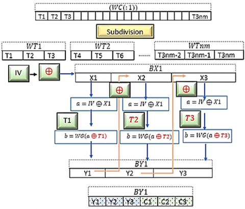
Steps 1 and 2: This first phase, depicted in Figures 11 and 12, consists of subdividing the original image and some Pseudo-Random vectors into sub-blocks of three pixels.
Steps 3, 4 and 5: The seed pixel is modified using an Initialization Value. Confusion/Diffusion: Perform the first internal confusion/diffusion operation on the block. (WC) Augmentation: The block is augmented by adding three Pseudo-Random values obtained from the table.
Figure 11. Subdividing the original image into sub-blocks
Figure 12. Pseudo-Random vectors to sub-blocks
Steps 6 and 7: These two steps are seen in Figure 13.
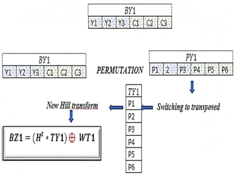
The permutation within the block is a displacement of rank $P D(i)$ or $P F(i)$ depending on the value of the binary control vector $B(: 1)$. The mathematical expressions of used parameters' permutation within a block is given in Table 12.
Figure 13. Sub-blocks permutation application
Table 12. Mathematical expressions of used parameters’ permutation within a block
|
Encryption Matrix |
|
$H=\left(\begin{array}{lll}a 1 & b 1 & c 1 \\ a 2 & b 2 & c 2 \\ a 3 & b 3 & c 3 \\ a 4 & b 4 & c 4 \\ a 5 & b 5 & c 5 \\ a 6 & b 6 & c 6\end{array}\right)$ So $H^t=\left(\begin{array}{llllll}a 1 & a 2 & a 3 & a 4 & a 5 & a 6 \\ b 1 & b 2 & b 3 & b 4 & b 5 & b 6 \\ c 1 & c 2 & c 3 & c 4 & c 5 & c 6\end{array}\right)$ |
|
New Encryption Formula |
|
$\left(\begin{array}{c}Z 1 \\ Z 2 \\ Z 3\end{array}\right)=\left(\begin{array}{llllll}a 1 & a 2 & a 3 & a 4 & a 5 & a 6 \\ b 1 & b 2 & b 3 & b 4 & b 5 & b 6 \\ c 1 & c 2 & c 3 & c 4 & c 5 & c 6\end{array}\right)\left(\begin{array}{c}P 1 \\ P 2 \\ P 3 \\ P 4 \\ P 5 \\ P 6\end{array}\right) \oplus\left(\begin{array}{c}T 1 \\ T 2 \\ T 3\end{array}\right)$ |
|
Outcome |
|
$\left\{\begin{array}{l}Z 1=\sum_{i=1}^6 a i * P i \oplus T 1 \\ Z 2=\sum_{i=1}^6 b i * P i \oplus T 2 \\ Z 3=\sum_{i=1}^6 c i * P i \oplus T 3\end{array}\right.$ |
Step 8: External diffusion.
With the support of the Pseudo-Random matrix (M) having dimension (3;3), whose is explained by the relation below, the diffusion process between the next clear block and the current cipher block is installed in this last encryption stage of development [18, 19]. Let (M) be the Pseudo-Random diffusion matrix, which is given in Figure 14.
Figure 14. Pseudo-Random diffusion matrix
2.5 Encrypted image decryption
We have developed a symmetric encryption technique. Consequently, throughout the decryption process [28-30], all encryption parameters will be employed utilizing reciprocal functions, beginning with the final encrypted block. The decryption procedure adheres to this timetable.
2.5.1 Reverse of the Hill method
$\left(\begin{array}{l}Z 1 \\ Z 2 \\ Z 3\end{array}\right)=H^t\left(\begin{array}{l}P 1 \\ P 2 \\ P 3 \\ P 4 \\ P 5 \\ P 6\end{array}\right) H\left(\begin{array}{l}Z 1 \\ Z 2 \\ Z 3\end{array}\right)=H H^t\left(\begin{array}{l}P 1 \\ P 2 \\ P 3 \\ P 4 \\ P 5 \\ P 6\end{array}\right)$
$H^t:$ a positive definite symmetric matrix, therefore invertible.
In effect:
$\begin{gathered}X H H^t X^t=(X H) *(X H)^t>0 \\ H\left(\begin{array}{l}Z 1 \\ Z 2 \\ Z 3\end{array}\right)=\mathrm{HH}^{\mathrm{t}}\left(\begin{array}{l}\mathrm{P} 1 \\ \mathrm{P} 2 \\ \mathrm{P} 3 \\ \mathrm{P} 4 \\ \mathrm{P} 5 \\ \mathrm{P} 6\end{array}\right) \\ \left(\begin{array}{l}\mathrm{P} 1 \\ \mathrm{P} 2 \\ \mathrm{P} 3 \\ \mathrm{P} 4 \\ \mathrm{P} 5 \\ \mathrm{P} 6\end{array}\right)=\left(\mathrm{HH}^{\mathrm{t}}\right)^{-1} * \mathrm{H} *\left(\begin{array}{l}\mathrm{Z} 1 \\ \mathrm{Z} 2 \\ \mathrm{Z} 3\end{array}\right)\end{gathered}$
Put $\mathrm{K}=\left(\mathrm{HH}^{\mathrm{t}}\right)^{-1} * \mathrm{H} \quad\left(\begin{array}{l}\mathrm{P} 1 \\ \mathrm{P} 2 \\ \mathrm{P} 3 \\ \mathrm{P} 4 \\ \mathrm{P} 5 \\ \mathrm{P} 6\end{array}\right)=\mathrm{K} *\left(\begin{array}{l}\mathrm{Z} 1 \\ \mathrm{Z} 2 \\ \mathrm{Z} 3\end{array}\right)$
2.5.2 S-Box decryption matrix
Generally speaking, any S-Box used in a cipher system can be reversed by Algorithm 19 to be used in the decryption process [20, 31]. An example is depicted in Table 13.
|
Algorithm 19: S-Box Decryption Matrix |
|
$\begin{aligned} & \text { for } \mathrm{k}=1 \text { to } \mathrm{t} \\ & \text { for } \mathrm{l}=1 \text { to } 256 \\ & \operatorname{SW} 1(\mathrm{k}, \operatorname{WS} 1(\mathrm{k} ; \mathrm{l}))=\mathrm{l} \\ & \operatorname{SW2}((\mathrm{k}, \operatorname{WS2}(\mathrm{k} ; \mathrm{l}))=1 \\ & \operatorname{Next} \mathrm{l}, \mathrm{k}\end{aligned}$ |
Table 13. S-Box decryption matrix example
|
(WS1) |
1 |
2 |
3 |
4 |
5 |
6 |
7 |
8 |
|
1 |
3 |
5 |
8 |
6 |
2 |
7 |
1 |
4 |
|
2 |
2 |
7 |
1 |
4 |
3 |
5 |
8 |
6 |
|
3 |
4 |
3 |
5 |
8 |
9 |
2 |
7 |
1 |
|
4 |
2 |
7 |
1 |
4 |
3 |
5 |
8 |
6 |
|
5 |
8 |
6 |
2 |
7 |
1 |
4 |
3 |
5 |
|
(SW1) |
1 |
2 |
3 |
4 |
5 |
6 |
7 |
8 |
|
1 |
7 |
5 |
1 |
8 |
2 |
4 |
6 |
3 |
|
2 |
3 |
1 |
5 |
4 |
6 |
8 |
2 |
7 |
|
3 |
8 |
6 |
2 |
1 |
3 |
5 |
7 |
4 |
|
4 |
3 |
1 |
5 |
4 |
6 |
8 |
2 |
7 |
|
5 |
5 |
3 |
7 |
6 |
8 |
2 |
4 |
1 |
We can obtain (x), by applying the same logic of Vigenere’s conventional technique using Algorithm 20.
|
Algorithm 20: Decryption Using Reverse S-Box Decryption Matrix |
|
if $z=\operatorname{SW} 1(y, x)$ Then $x=\operatorname{WS} 1(y, z)$ |
This formula allows us to recalculate the reciprocal function of the confusion function using the two S-Boxes.
This novel encryption employs an involutive diffusion function, as depicted in Algorithm 21. It is consequently comparable to its reciprocal.
|
Algorithm 21: Decryption process using the confusion reciprocal function |
|
1. $\operatorname{WG}(\mathrm{Y}(\mathrm{i}))=\mathrm{X}(\mathrm{i})$ 2. if $\mathrm{WB}(\mathrm{i} ; 2)=0$ then 3. $\begin{aligned} X(i)=\text { SW2(WC(i; 3); SW1(WC((i; 2), Y(i) } \oplus W C(i ; 5)) \oplus W C(i ; 1)\end{aligned}$ 4. $X(i)=W S 1(W C(i ; 2) ; \operatorname{SW}1(W C((i ; 2), Y(i) \oplus \mathrm{WC}(\mathrm{i} ; 5)) \oplus \mathrm{WC}(\mathrm{i} ; 5)$ |
The diffusion function is, by construction, an involutive function; consequently, it is identical to its reciprocal.
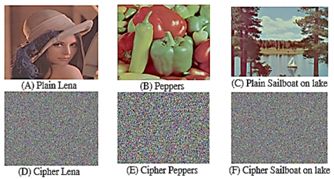
In this section, we extract a large selection of images from a reference dataset [32], that will be used to evaluate the performance of our new algorithm. The results obtained will be presented and compared to those of other existing approaches. The robustness of a cipher scheme is judged by its ability to resist known attacks. A subset of reference images, processed by our algorithm, is presented in Figure 15.
Figure 15. Image examples tested by our new algorithm
3.1 The analysis of the key space
A brute force assault is a cryptanalysis procedure used to discover the cipher key by systematically trying all possible combinations. Consequently, a larger cipher key can make brute-force assaults impractical. For the case of our system, the secret key size exceeds (2192), ensuring enhanced protection against brute force attacks. We declare that our secret key is generated using the three most used chaotic maps in cryptography. However, it comprises six parameters, each written in 32 bits, resulting in an overall size $\left(2^{6 * 32}\right)=\left(2^{192}\right) \gg\left(2^{100}\right)$.
3.2 Secret key’s sensitivity analysis
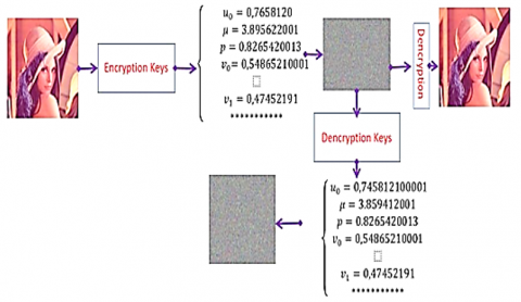
The chaotic maps used in our algorithm have a high sensitivity to the initial conditions. Therefore, any perturbation, even a small one, of a parameter during the secret key regeneration, can generate distinct chaotic vectors. Figure 16 illustrates the high sensitivity of the key of our new technology.
We find that a small alteration of any parameter, of the order of 10-6 can lead to not being able to restore the plain image.
Figure 16. The encryption key sensitivity
3.3 Statistics attack security
To assess the robustness of our new medical and color image encryption technique against statistical attacks, we conducted a series of tests on a set of images. Here, we present the results of the most significant tests.
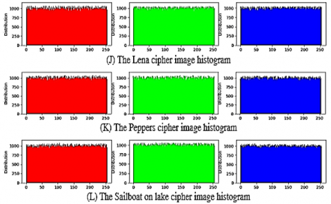
3.3.1 The analysis of histograms
An image histogram is a graphical representation of the gray level distribution. The x-axis represents the set of color levels, ranging from 0 to 255, while the height of each vertical bar indicates the frequency of occurrence of a specific color level in the image. In cryptography, an encrypted image's color distribution is important since it may provide details about the original image. Conversely, if the histogram of the encrypted image is flat and uniform, this may provide no information about the original image or the relationship between the two.
Some simulation results of our system are shown in Figure 15 (G-H-I: for plain images histograms) and (J-K-L: for cipher images histograms).
In the context of this study, we note that all the reference images encrypted by our algorithm exhibit a uniformly distributed histogram. This property provides increased protection against histogram analysis attacks.
3.3.2 The analysis of entropy
The relation that explains the entropy between the pixels of an image is given by Eq. (6).
$H(M C)=\frac{1}{s} \sum_{j=1}^s-p(j) \log _2(p(j))$ (6)
Table 14. Encrypted images entropy by our method
|
Image |
Cipher Images Entropy |
||
|
R |
G |
B |
|
|
Lena |
7,9997 |
7,9996 |
7,9995 |
|
Peppers |
7,9996 |
7,9997 |
7,9995 |
|
Sailboat |
7.9998 |
7,9997 |
7,9996 |
p(j): the probability of occurrence of level (j) in the plain image. Table 14 shows the results of the tested images by our scheme.
3.3.3 The analysis of correlation
A technique used to compare two images; correlation helps estimate the displacement of pixels in one image relative to another reference image. The relevant expression for this technique, correlation, is defined by Eq. (7).
$\rho=\frac{\operatorname{cov}(x 1, x 2)}{\sqrt{V(x 1)} \sqrt{V(x 2)}}$ (7)
We notice that the value of the correlation is close to zero, which guarantees a better protection against correlation attacks. Each pixel in the original image is highly correlated with its neighboring pixels in the horizontal, vertical, or diagonal directions. This correlation contains information that an attacker could exploit to reconstruct the original image. A strong encryption system should minimize this correlation as much as possible, ideally reducing it to zero. As depicted in Table 15, the correlation values of images encrypted using our approach are close to zero, confirming that our system is effective against statistical and frequency attacks.
Table 15. Correlation coefficients
|
Name |
Original Images |
Encrypted Images |
|||||
|
Horizontal |
Vertical |
Diagonal |
Horizontal |
Vertical |
Diagonal |
||
|
Lena |
R |
0.982726 |
0.988578 |
0.972728 |
-0.00161 |
0.002177 |
-0.007733 |
|
G |
0.992783 |
0.972065 |
0.974490 |
0.00108 |
-0.01832 |
-0.002432 |
|
|
B |
0.977263 |
0.974761 |
0.980021 |
0.001936 |
0.004860 |
0.007052 |
|
|
Peppers |
R |
0.986795 |
0.974727 |
0.976397 |
-0.00867 |
0.008771 |
0.007611 |
|
G |
0.976447 |
0.984192 |
0.977354 |
0.007323 |
0.032642 |
0.004711 |
|
|
B |
0.986065 |
0.981639 |
0.971148 |
-0.01778 |
0.036201 |
0.021560 |
|
3.3.4 Differential analysis
This section studies the behavior of the differential metrics, such as the UACI, NPCR, and the avalanche effect, which must be studied. Let be two encrypted images, whose corresponding free-to-air images differ by only one pixel, from (C1) and (C2), respectively. The ![]() mathematical analysis of an image is given by the Eq. (8).
mathematical analysis of an image is given by the Eq. (8).
$N P C R=\left(\frac{1}{3 n m} \sum_{j, k=1}^{3 n m} D(j, k)\right) * 100$ (8)
With $D(\mathrm{j}, \mathrm{k})=\left\{\begin{array}{lll}1 & \text { if } & \mathrm{C}_1(\mathrm{j}, \mathrm{k}) \neq \mathrm{C}_2(\mathrm{j}, \mathrm{k}) \\ 0 & \text { if } & \mathrm{C}_1(\mathrm{j}, \mathrm{k})=\mathrm{C}_2(\mathrm{j}, \mathrm{k})\end{array}\right.$
The mathematical analysis of the UACI for an image is given by Eq. (9).
$U A C I=\left(\frac{1}{n m} \sum_{j, k=1}^{3 n m} A b s\left(C_1(j, k)-C_2(j, k)\right)\right)$ (9)
The avalanche effect is a key feature of almost all cryptographic hash functions and block cipher algorithms. It causes increasingly significant changes as data flows through the algorithm’s framework. This constant determines the avalanche impact of the cryptographic system being utilized. The value is approximated by Eq. (10).
As depicted in Table 16, the values of the differential for the reference images tested with our new technology align with universal standards. At this point, the NPCR value is nearly 99.99%, and the UACI value surpasses 33.34%. This guarantees that our encryption system is resistant to differential attacks. This protection arises from the implementation of the initial round. The avalanche effect values from the images tested with our technology offer robust defense against differential attacks.
$A E=\left(\frac{\sum_i \text { bit change }}{\sum_i \text { bit total }}\right) * 100$ (10)
Table 16. The NPCR, UACI and avalanche effect results
|
Encrypted Images |
NPCR_% |
UACI_% |
Avalanche Effect |
||||
|
R |
G |
B |
R |
G |
B |
||
|
Lena |
99.69 |
99.74 |
99.66 |
33.49 |
33.50 |
33.58 |
51.03 |
|
Peppers |
99.70 |
99.65 |
99.72 |
33.48 |
33.49 |
33.57 |
50.24 |
3.4 Comparison
Based on the findings of each algorithm's security study, we will evaluate the performance of our method against several alternative approaches in Table 16, this comparison demonstrates our cryptosystem's resilience to all known threats.
3.5 Discussion
Through simulations on a variety of reference pictures, including Lena and Plain Peppers, our encryption method has been thoroughly assessed, demonstrating its resilience to known attacks and robustness. The incredibly pleasing outcomes attained validate our system's functionality and inspire researchers to make more advancements. Moreover, a careful comparison with other comparable systems indicates minor security. advantage, which boosts trust in our system's ability to protect sensitive data that is vast, extremely redundant, and highly correlated. These encouraging results push for wider validation and use of our encryption technology.
The chaotic maps produced by our research exhibit an extraordinary sensitivity to initial conditions. Furthermore, because our private key is so big, the system is protected from brute force attacks [18]. The randomness introduced by the permutation further adds to the potential attack’s complexity. At last, strong chaining mechanisms installed in both towers provide protection against known attacks against the new encryption method.
4.1 The benefits of the process
Our approach is suitable for images of all sizes and formats. Non-commutative algebraic operations enhance the system's robustness. The Pseudo-Random size of the substitution table makes it more difficult to reconstruct the employed S-Boxes. The structure of the S-Box, combined with its operation governed by a chaotic decision vector, adds further complexity to attacking our method. Moreover, encryption keys generated from chaotic maps are extremely sensitive to initial conditions, making it hard to retrieve the actual key employed.
4.2 The approach restrictions
The restrictions of our methodology are mostly dictated by the bounds of the S-Box building and chaotic map selection processes, in addition to the Pseudo-Random size of the S-Boxes that are formed.
Our work on the weaknesses in current color image encryption systems, especially the limits of older Hill and Vigenère methods, has led to a major breakthrough. We didn't just tweak existing standards; we fundamentally reimagined them for today's security needs. By using a pseudorandom non-square encryption matrix and cleverly blending enhanced Hill and Vigenère principles, we've built a system that beats the old statistical and linear vulnerabilities. Our tests on many images from different databases show clear results. They prove our method is both consistent and strong, and that it can effectively stop brute-force attacks by making them incredibly time-consuming. It's no longer about if a coded image can be broken, but about the exponential difficulty our method creates for any attacker. This new algorithm opens up exciting possibilities for keeping sensitive visual data safe in our increasingly digital world. Whether for military messages, medical images, or personal privacy, our solution adds a vital layer of protection. We believe this is a big step towards truly private and tough visual communication. The time of easily hackable digital images is ending, giving way to an era where security is built right into how we handle visual information.
[1] Aberna, P., Agilandeeswari, L. (2024). Digital image and video watermarking: Methodologies, attacks, applications, and future directions. Multimedia Tools and Applications, 83(2): 5531-5591. https://doi.org/10.1007/s11042-023-15806-y
[2] Bansal, R., Gupta, S., Sharma, G. (2017). An innovative image encryption scheme based on chaotic map and Vigenère scheme. Multimedia Tools and Applications, 76(15): 16529-16562. https://doi.org/10.1007/s11042-016-3926-9
[3] Belgarric, P., Bhasin, S., Bruneau, N., Danger, J.L., et al. (2013). Time-frequency analysis for second-order attacks. In International Conference on Smart Card Research and Advanced Applications, pp. 108-122. https://doi.org/10.1007/978-3-319-08302-5_8
[4] El Bourakkadi, H., Chemlal, A., Tabti, H., Kattass, M., et al. (2024). Improved Vigenere approach incorporating pseudorandom affine functions for encrypting color images. International Journal of Electrical and Computer Engineering, 14(3): 2684-2694. http://doi.org/10.11591/ijece.v14i3.pp2684-2694
[5] Chatterjee, D., Banik, B.G., Banik, A. (2023). Attack resistant chaos-based cryptosystem by modified baker map and logistic map. International Journal of Information and Computer Security, 20(1-2): 48-83. https://doi.org/10.1504/IJICS.2023.128002
[6] Chen, Y., Xie, R., Zhang, H., Li, D., et al. (2024). Generation of high-order random key matrix for Hill Cipher encryption using the modular multiplicative inverse of triangular matrices. Wireless Networks, 30(6): 5697-5707. https://doi.org/10.1007/s11276-023-03330-8
[7] Fan, W., Li, T., Wu, J., Wu, J. (2023). Chaotic color image encryption based on eight-base DNA-level permutation and diffusion. Entropy, 25(9): 1268. https://doi.org/10.3390/e25091268
[8] Hadj Brahim, A., Ali Pacha, A., Hadj Said, N. (2024). An image encryption scheme based on a modified AES algorithm by using a variable S-Box. Journal of Optics, 53(2): 1170-1185. https://doi.org/10.1007/s12596-023-01232-8
[9] JarJar, A. (2021). New chaotic map development and its application in encrypted color image. Journal of Multimedia Information System, 8(2): 131-142. https://doi.org/10.33851/JMIS.2021.8.2.131
[10] Kadir, A., Hamdulla, A., Guo, W.Q. (2014). Color image encryption using skew tent map and hyper chaotic system of 6th-order CNN. Optik, 125(5): 1671-1675. https://doi.org/10.1016/j.ijleo.2013.09.040
[11] Kundu, A., Das, J.C., Debnath, B., De, D., et al. (2024). Design of reversible quantum Vigenere cryptographic cipher in QCA and IBMQ platforms for secure noncommunication. Nano, 19(3): 2450013. https://doi.org/10.1142/S1793292024500139
[12] Liu, Q., Liu, L. (2020). Color image encryption algorithm based on DNA coding and double chaos system. IEEE Access, 8: 83596-83610. https://doi.org/10.1109/ACCESS.2020.2991420
[13] Liu, X., Xiao, D., Xiang, Y. (2018). Quantum image encryption using intra and inter bit permutation based on logistic map. IEEE Access, 7: 6937-6946. https://doi.org/10.1109/ACCESS.2018.2889896
[14] Lone, M.A., Qureshi, S. (2022). RGB image encryption based on symmetric keys using Arnold transform, 3D chaotic map and affine hill cipher. Optik, 260: 168880. https://doi.org/10.1016/j.ijleo.2022.168880
[15] Lu, J., Zhang, J., An, D., Hao, D., et al. (2024). A low-time-consumption image encryption combining 2D parametric Pascal matrix chaotic system and elementary operation. Journal of King Saud University-Computer and Information Sciences, 36(8): 102169. https://doi.org/10.1016/j.jksuci.2024.102169
[16] Luo, Y., Yu, J., Lai, W., Liu, L. (2019). A novel chaotic image encryption algorithm based on improved baker map and logistic map. Multimedia Tools and Applications, 78(15): 22023-22043. https://doi.org/10.1007/s11042-019-7453-3
[17] Hong, Y., Fang, S., Su, J., Xu, W., et al. (2023). A novel approach for image encryption with Chaos-RNA. Computers, Materials & Continua, 77(1): 139-160. https://doi.org/10.32604/cmc.2023.043424
[18] Toktas, F., Erkan, U., Yetgin, Z. (2024). Cross-channel color image encryption through 2D hyperchaotic hybrid map of optimization test functions. Expert Systems with Applications, 249: 123583. https://doi.org/10.1016/j.eswa.2024.123583
[19] Umar, T., Nadeem, M., Anwer, F. (2024). A new modified skew tent map and its application in Pseudo-Random number generator. Computer Standards Interfaces, 89: 103826. https://doi.org/10.1016/j.csi.2023.103826
[20] Vaidyanathan, S., Kammogne, A.S.T., Tlelo-Cuautle, E., Talonang, C.N., et al. (2023). A novel 3-D jerk system, its bifurcation analysis, electronic circuit design and a cryptographic application. Electronics, 12(13): 2818. https://doi.org/10.3390/electronics12132818
[21] Boussif, M., Mnassri, A. (2022). Secure images transmission using a three-dimensional S-Box-based encryption algorithm. In 2022 5th International Conference on Advanced Systems and Emergent Technologies (IC_ASET), Hammamet, Tunisia, pp. 17-22. https://doi.org/10.1109/IC_ASET53395.2022.9765904
[22] Belazi, A., Khan, M., El-Latif, A.A.A., Belghith, S. (2017). Efficient cryptosystem approaches: S-Boxes and permutation–substitution-based encryption. Nonlinear Dynamics, 87(1): 337-361. https://doi.org/10.1007/s11071-016-3046-0
[23] Naim, M., Pacha, A.A. (2023). A novel image encryption algorithm based on advanced hill cipher and 6D hyperchaotic system. International Journal of Network Security, 25(5): 829-840. https://doi.org/10.6633/IJNS.202309_25(5).13
[24] Song, W., Fu, C., Zheng, Y., Zhang, Y., Chen, J., Wang, P. (2024). Batch image encryption using cross image permutation and diffusion. Journal of Information Security and Applications, 80: 103686. https://doi.org/10.1016/j.jisa.2023.103686
[25] Kanwal, S., Inam, S., Shah, A.A., Iqbal, H., et al. (2024). A robust approach to satellite image encryption using chaotic map and circulant matrices. Engineering Reports, 6(12): e13010. https://doi.org/10.1002/eng2.13010
[26] Mehdi, S.A., Kadhim, A.A. (2019). Image encryption algorithm based on a new five dimensional hyperchaotic system and Sudoku matrix. In 2019 international engineering conference (IEC), Erbil, Iraq, pp. 188-193. https://doi.org/10.1109/IEC47844.2019.8950560
[27] Tabti, H., El Bourakkadi, H., Chemlal, A., Jarjar, A., et al. (2024). Novel cryptosystem integrating the Vigenere cipher and one Feistel round for color image encryption. International Journal of Electrical Computer Engineering (IJECE), 14(5): 5701-5714. http://doi.org/10.11591/ijece.v14i5.pp5701-5714
[28] Weber, A. (2018). The USC-SIPI image database, 2014. http://sipi.usc.edu/database.
[29] Fu, C., Chen, J.J., Zou, H., Meng, W.H., et al. (2012). A chaos-based digital image encryption scheme with an improved diffusion strategy. Optics Express, 20(3): 2363-2378. https://doi.org/10.1364/OE.20.002363
[30] Winarno, E., Nugroho, K., Adi, P.W., Setiadi, D.R.I.M. (2023). Combined interleaved pattern to improve confusion-diffusion image encryption based on hyperchaotic system. IEEE Access, 11: 69005-69021. https://doi.org/10.1109/ACCESS.2023.3285481
[31] Wang, Y., Leng, X., Zhang, C., Du, B. (2023). Adaptive fast image encryption algorithm based on three-dimensional chaotic system. Entropy, 25(10): 1399. https://doi.org/10.3390/e25101399
[32] Li, T., Shi, J., Zhang, D. (2021). Color image encryption based on joint permutation and diffusion. Journal of Electronic Imaging, 30(1): 013008. https://doi.org/10.1117/1.JEI.30.1.013008