Nawel Bendimerad*![]() | Amal Boumedjout
| Amal Boumedjout![]() | Bena Bot
| Bena Bot![]()
© 2024 The authors. This article is published by IIETA and is licensed under the CC BY 4.0 license (http://creativecommons.org/licenses/by/4.0/).
OPEN ACCESS
Directional sensor networks (DSNs) have possibility to provide more precise surveillance than conventional omni-directional sensor networks since the captured data can be of a visual nature. Therefore, the coverage problem in DSNs is completely different from that of traditional scalar sensors. Barrier coverage is a specific type of coverage that is emerged in DSNs to ensure a high-level monitoring application. In this paper, we focus on solving the barrier coverage problem in hybrid DSNs using stationary and mobile directional sensors. Our aim is to ensure a high barrier coverage specially developed for surveillance applications by proposing two approaches. In the first one, we implement a distributed algorithm based on a geometric mathematical model to calculate the new orientation of directional sensors to maximize barrier coverage. The purpose of using a geometric mathematical model is to compute, after a random deployment, the most appropriate angle of rotation for each directional sensor so that the novel DSN configuration ensures a high level of intrusion detection across the barrier. In the second one, we enhance the first approach by extending its algorithm to further improve barrier coverage using mobile directional sensors deployed far from the barrier. This solution allows us to achieve a strong barrier coverage with a minimum number of active directional sensors. Extensive simulation experiments with different scenarios are conducted to show the effectiveness of the proposed algorithms in hybrid DSNs, such as those varying the number of stationary and mobile directional sensors with different angles of view.
barrier coverage, hybrid directional sensor networks, mobile directional sensors, surveillance applications, stationary directional sensors
In the last decade, directional sensor networks (DSNs) have become very popular due to their promising surveillance applications of wireless sensor networks (WSN) [1] such as environmental monitoring, disaster response, battlefield surveillance, etc. A DSN is considered as a WSN composed of directional sensors, such as ultrasound, infrared and video sensors [2]. The main difference between DSNs and traditional wireless sensor networks is that the sensed data by directional sensors are in the form of images or videos. This quality of data can provide much richer information about the environment and more precise surveillance than the one offered by scalar sensors. Therefore, because of the nature of the sensed data, the coverage problem becomes more complex in DSN compared to WSN. Unlike conventional omni-directional sensors that always have an omni-angle of sensing range, a directional sensor can ensure coverage of just a sector of the covered area [3]. Therefore, to have an efficient coverage in a DSN, we have to take into consideration the sensing range and the angle of view (AoV) of each directional sensor.
The coverage problem in DSNs can be divided into three categories: target coverage, area coverage, and barrier coverage. The aim of the target coverage is to determine a subset of directional sensors to cover a set of targets [4, 5]. The area coverage is related to the field coverage [6-8], where directional sensors are activated in such a way to ensure a full region coverage. In the barrier coverage, the main objective is to have the ability to detect intrusion crossing a barrier of directional sensors [9]. It can be classified into weak barrier and strong barrier coverage explained in subsection 3.2. In this paper, we address the barrier coverage problem for both weak and strong barrier coverage.
Barrier coverage can be used for various security applications, such as border protection, dangerous substance monitoring and critical resource protection. There are many challenging issues to ensure barrier coverage for security applications using DSN. First, since the area of interest is hard to reach, random deployment of directional sensors by air-plane or other methods is commonly used, making the location and direction of sensors unpredictable. In this case, an adequate configuration of the directional sensors initially deployed in the surveillance area is necessary to achieve efficient barrier coverage. Second, due to the cost and energy constraints of sensors, we don’t have possibility to use solely mobile directional sensors in the network. Therefore, in this work, we consider a hybrid DSN with a two-phase deployment strategy. The first phase concerns only the stationary directional sensors deployment. Subsequently, we deploy a fraction of mobile directional sensors in the second phase. This hybrid approach using stationary and mobile directional sensors allows us to maximize the efficiency of the barrier coverage, while extending the network lifetime by the scheduling strategy of directional sensors’ activity.
In this paper, our main goal is divided into two parts. In the first part of our contribution, after the initial random deployment phase, we calculate the adequate working direction of each sensor that the position is near the barrier. To compute the new orientation of directional sensors, we designed a distributed algorithm based on a new geometric mathematical model that allows us to achieve a weak barrier coverage. In the second part of our contribution, we further proposed an enhancement of the above-mentioned approach by exploiting mobile directional sensors whose position is far from the barrier. Changing the position of mobile directional sensors allows us in one hand to generate more redundant directional sensors in the network in order to keep a lower number of sensors in active mode and therefore to increase the network lifetime. In other hand, the new sensing direction of mobile directional sensors gives us the ability to reinforce the barrier coverage to finally achieve a strong barrier coverage.
The remainder of this paper is organized as follows; In Section 2, related work is briefly summarized. In Section 3, firstly, we describe the directional sensor node model, then we give a definition of the barrier coverage and finally, we present our two approaches which concern the weak and strong barrier coverage with the corresponding algorithms. A series of simulation results are given in Section 4, and Section 5 concludes the paper.
Barrier coverage was first studied using WSN. Different approaches were proposed in the studies of Kumar et al. [10], Liu et al. [11], and Chen et al. [12, 13], that employed only stationary omni-directional sensors. Recently, sensor mobility was also exploited to improve the barrier coverage. The main proposals in this field that focused on mobile omni-directional sensors are presented by Fan et al. [14], Li and Liu [15], Chakraborty and Rout [16], Cheng et al. [17], and Yao et al. [18]. However, in this paper, we are solely interested in enhancing barrier coverage through stationary and mobile directional sensors.
Several approaches have been proposed in the literature to solve the barrier coverage problem in DSNs using stationary directional sensors. Khanjary et al. [19] suggested a distributed learning automata to find strong barrier lines in adjustable-orientation directional sensor networks by proposing a centralized and a distributed algorithm. Binh et al. [20] proposed a solution to the barrier coverage problem under a uniform random deployment scheme based on a new (k-ω) coverage model. To solve the problem, the authors presented an efficient method called Dynamic Partition. Chen et al. [21] proposed a solution to the barrier gap problem in weak and strong barrier coverage. To mend barrier gaps in the network, they present two gap-mending algorithms using sensor rotation that can fix barrier gaps and improve the probability of barrier success construction. The authors Cheng and Hsu [22], employed the virtual target-barrier construction (VTBC) method. To convert the complicated target-barrier construction problem in a rotatable DSN into a simpler optimization problem, authors defined and calculated a virtual barrier curve. Binh et al. [23] also investigated the strong barrier coverage problem by maximizing the network lifetime. They proposed a Modified Maximum Flow Algorithm (MMFA) using heterogeneous wireless turnable camera sensor networks. Hong et al. [24] have recently studied the problem of strong barrier coverage in 3D camera sensor networks, which aim to monitor intruders in irregular spaces with high resolution and maximize the network lifetime.
Among the existing works that studied barrier coverage for DSN with mobile sensors, we can mention Wang et al. [25], who investigated a k-barrier coverage by using mobile directional sensors. The authors introduced a novel concept of weighted barrier graph (WBG) and proposed an optimal and a greedy solution to the problem. The strength of this approach is that the authors determined the minimum number of mobile directional sensors required to form a k-barrier coverage and to minimize cost. Unlike this work, in our proposal, we take advantage of redundant sensors generated by overlapping sensing regions, which are suitable for barrier coverage. The purpose of this configuration is to minimize energy consumption or replace a failed sensor whose angle of view is already covered by its neighbors.
Liu et al. [26] studied how to efficiently improve barrier coverage using mobile camera sensors. In this work, the authors used a grid-based strategy for camera sensors deployment and employed Dijkstra’s algorithm to obtain the shortest camera barrier. Different from our work, where redundant sensors are exploited to ensure a strong barrier coverage and also to save energy, the solution proposed by Liu et al. [26] made use of redundant camera sensors just to achieve full-view coverage.
In the study presented by Zhao et al. [27], an energy-efficient barrier coverage was proposed for DSNs with mobile sensors, where a flow graph is constructed based on the sensor location in formation and then the maximum flow of the flow graph is computed. The authors developed an interesting energy-efficient barrier repair algorithm to improve the barrier coverage. However, in this work, the barrier coverage problem was converted to a bond percolation model. Whereas, in our new proposal, the barrier coverage is improved by using a configuration algorithm executed in a distributed manner with a reduction of the computational complexity.
The work presented by Liu et al. [28] used the same deployment strategy proposed by Liu et al. [26], which focused on a grid-based deployment strategy and a graph-based algorithm to obtain a full-view coverage barrier that can capture multiple viewpoints of the target crossing the protected area.
In this paper, we also explore the barrier coverage problem, which can be categorized into weak and strong barrier coverage. The former aims to detect the majority of intruders through the barrier, while the latter must ensure the detection of all intruders regardless of how they cross.
Unlike the above-mentioned studies on barrier coverage, our proposed solution considers benefits of hybrid DSNs by using a two-phase deployment. Therefore, in this paper, the deployment strategy is completely different from the one presented in the previous studies [25-28]. First, stationary directional sensors that can only change orientation are randomly deployed in the barrier area. Second, the sensor deployment is completed by mobile directional sensors that are capable of changing orientation and even position. The main objective of the second deployment is to reinforce the coverage already ensured by the stationary sensors.
The proposed solution in this paper is based on a new geometric mathematical model that allows us to calculate an angle of rotation for each directional sensor to obtain a novel configuration of their orientation. These directional sensors must be arranged to form a virtual barrier horizontally along the area of interest in order to provide effective barrier coverage after a random deployment. The mobility function of mobile directional sensors is also exploited to obtain more redundant sensors. This helps detect any intruders moving along crossing paths, ensuring they are monitored simultaneously by multiple directional sensors for more accurate detection. This second contribution allows us to ensure a strong barrier coverage suitable for surveillance applications and to extend the network lifetime.
In this section, we present a detailed description of the barrier coverage problem and our proposed solutions to this problem. At first, we start by a definition of the directional sensor node model to give an idea about a sensing region in DSNs. Then, we explain the difference between the weak barrier coverage and the strong barrier coverage problem. Finally, we present our contributions on the barrier coverage problem already defined by proposing two approaches using directional and mobile sensors. The first contribution considers the weak barrier coverage and the second one investigates the strong barrier coverage.
3.1 Directional sensor node model
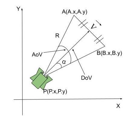
The directional sensor node model illustrated in this subsection, is based on a geometric mathematical model inspired by the one presented in the study of Bendimerad and Kechar [7]. As shown in Figure 1 the sensing region of a directional sensor is defined as a sector, which can be approximated by an isosceles triangle. Then, we have three vertices, P, A and B, where P (P.x, P.y) is the current position of the sensor. The sector of each sensor is characterized by the following parameters: an angle of view (AoV) that is equal to 2 α as illustrated in Figure 1, a sensing radius R, a depth of view (DoV), and an orientation vector $\overrightarrow{V}$, which is the center line of sight of the AoV.
Figure 1. Directional sensor node model
In this paper, we have exploited this directional sensor node model in order to maximize the barrier coverage. Our main goal is to compute the appropriate direction and position of each stationary or mobile directional sensor using a new geometric mathematical model. Detailed descriptions of the different steps used by these stationary and mobile directional sensors, based on the executed distributed algorithms, are presented in the subsections 3.3 and 3.4.
3.2 Barrier coverage problem
Barrier coverage is one of the main applications of DSN to ensure intruder detection and surveillance. It is defined as the DSN capacity to detect intruders that attempt to cross the region of interest [27]. The aim of the barrier coverage is to avoid undetected penetration through the conceptual barrier formed by directional sensors.
We can find two kinds of barrier coverage: weak barrier coverage and strong barrier coverage.
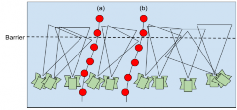
Weak barrier coverage requires that the union of sensors form a barrier in the horizontal direction from the left to the right boundary, so that every intruder moving along congruent crossing paths can be detected. We can see from Figure 2 an example of weak barrier coverage where it is possible to have two paths (a) and (b), which are not covered by directional sensors.
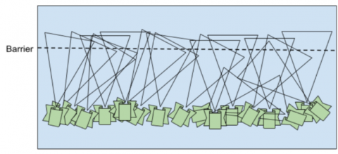
In strong barrier coverage, we have to verify that every intruder can be detected no matter what crossing path it takes. As shown in Figure 3, directional sensors provide a strong barrier coverage, since any intruder can be detected by the barrier on the top.
Figure 2. Weak barrier coverage example
Figure 3. Strong barrier coverage example
3.3 Proposed solution to the weak barrier coverage problem
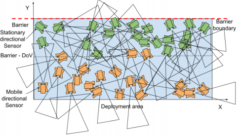
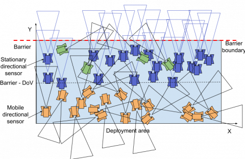
In this subsection, we present our first contribution, where we exploit solely the change in orientation of the directional sensors that are in the vicinity of the barrier. In this proposal, we have made the following assumptions (see Figure 4):
• We consider a hybrid DSN with a two-phase deployment strategy. Half of the total number of directional sensors, which are first randomly deployed close to the barrier region, are stationary. The second half of the deployed sensors in the barrier area concerns mobile directional sensors.
• All directional sensors have rotational capability to change orientation.
• The monitoring area is limited by a barrier indicated by a red dashed line on the top of the figure.
Figure 4. Random deployment of directional sensors
All directional sensors are randomly deployed in the vicinity of the barrier in a two-dimensional Euclidean plane with the same parameters.
As illustrated in Figure 4, since each directional sensor also has an arbitrary working direction and position, we cannot have all sensors in front of the barrier to reach a satisfactory barrier coverage.
The different steps of our distributed algorithm by considering the directional sensor node model presented in the first subsection, are as follows:
At first, we have to take into consideration directional sensors that the position is between the already defined value of the barrier and the value “Barrier-DoV” (shown in Figure 4). The purpose of this condition is to verify if the working direction of the sensor is not in front of the barrier (see Algorithm 1, line 1).
If the above condition is verified, we determine in which direction the sensor is oriented.
Finally, we adjust orientation of the directional sensors with an angle of rotation (AR) computed in the algorithm.
By using the angle α and coordinates of points P, A and B, as defined in the directional sensor node model, the main idea to calculate the angle of rotation (AR) explained in the algorithm 1 is as follows:
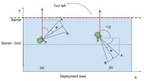
If the directional sensor has to turn left, we have to take into consideration for example one of the following two cases in order to use the adequate geometry formulas with “sign=-1” of AR (illustrated in Algorithm 1, lines 2-10 and Figure 5):
• Case a: If the sensor is directed to the right in the upper part (see Figure 5(a)), we apply the following geometry formula:
$A R=\alpha+\cos ^{-1} \frac{A \cdot \mathrm{y}-\mathrm{P} . \mathrm{y}}{\|\overrightarrow{P A}\|}$ (1)
• Case b: If the sensor is directed to the right in the lower part (see Figure 5(b)), we apply the following geometry formula:
$A R=\alpha+\sin ^{-1} \frac{\mathrm{A} \cdot \mathrm{y}-\mathrm{P} \cdot \mathrm{y}}{\|\overrightarrow{P A}\|}+\frac{\pi}{2}$ (2)
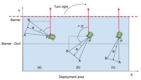
If the directional sensor has to turn right, we have to take into consideration for example one of the following three cases in order to use the adequate geometry formulas with “sign=+1” of AR (illustrated in Algorithm 1, lines 11-23 and Figure 6):
• Case a: If the sensor is directed to the left in the upper part (see Figure 6(a)), we apply the following geometry formula:
$A R=\alpha+\cos ^{-1} \frac{B \cdot \mathrm{y}-\mathrm{P} \cdot \mathrm{y}}{\|\overrightarrow{P B}\|}$ (3)
• Case b: If the sensor is directed to the left in the lower part (see Figure 6(b)), we apply the following geometry formula:
$A R=\alpha+\sin ^{-1} \frac{\mathrm{B} \cdot \mathrm{y}-\mathrm{P} \cdot \mathrm{y}}{\|\overrightarrow{P B}\|}+\frac{\pi}{2}$ (4)
• Case c: If the sensor is pointing down (see Figure 6(c)), we apply the following geometry formula:
$A R=\pi-\alpha$ (5)
Figure 5. Cases when a directional sensor has to turn left
Figure 6. Cases when a directional sensor has to turn right
|
Algorithm 1 Orientation Adjustment |
|
Require: P(P.x,P.y), A(A.x,A.y), B(B.x,B.y), α , DoV, Barrier; Ensure: AR;
|
Figure 7. Directional sensors after applying the orientation adjustment algorithm
After applying the algorithm of orientation adjustment, the new direction of each selected sensor that the position is between the barrier and the value “Barrier-DoV” is shown in blue color in Figure 7. It can be seen from this figure that barrier coverage is maximized after changing orientation of directional sensors compared to the sensor deployment shown in Figure 4.
3.4 Proposed solution to the strong barrier coverage problem
The aim of our second contribution is to improve the first proposal by taking into consideration mobile directional sensors that are far from the barrier. In this approach, we exploit on one hand mobility function of the selected directional sensors by changing their position in order to reach and to cover the barrier. On another hand, we apply the algorithm illustrated in the previous subsection to optimize the working direction of the mobile directional sensors to achieve a strong barrier coverage. Furthermore, we have taken advantage of some redundant directional sensors that may exist on the barrier. The scheduling strategy of directional sensors’ activity allow us to prolong the network lifetime and to ensure coverage of failed sensors.
The different steps of our extended algorithm (summarized in Algorithm 2) to achieve a strong barrier coverage by considering the directional sensor node model presented in the subsection 3.1 are as follows:
At first, we have to determine which are mobile directional sensors whose position is below the value “Barrier-DoV” (as shown in Figure 4). The purpose of this condition is to verify that the sensor position is far from the barrier (see Algorithm 2, line 1).
If the above condition is verified, we activate sensor’s mobility function and we change coordinates of the sensor position to reach the barrier (see Algorithm 2, lines 2-4). Then, Algorithm 1 is used for orientation adjustment in order to have all sensors’ direction in front of the barrier.
After a neighborhood discovery, the sensor verifies if its AoV is already covered by a neighbor sensor (see Algorithm 2, lines 8-13), in which case the concerned directional sensor can turn to inactive mode in order to minimize energy consumption or replace a failed sensor.
|
Algorithm 2 Position Adjustment |
|
Require: P(P.x,P.y), DoV, Barrier, Barrier_boundary, N(S): the set of the neighbors called S’ of the sensor S; Ensure: P’(P’.x,P’.y), AR, S.activity;
|
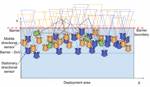
After applying the algorithm of position adjustment, the new position and direction of the selected mobile directional sensors is shown in orange color in Figure 8. Compared with the sensor deployment shown in Figure 4, we can see from Figure 8 that barrier coverage is maximized after changing orientation and position of mobile directional sensors to finally reach a strong barrier coverage.
Figure 8. Directional sensors after applying the position adjustment algorithm
In this section, we present the experimental results of the following algorithms:
• DSN_WBC (Directional sensor network for weak barrier coverage), where it is possible to change only the sensors’ orientation.
• DSN_SBC (Directional sensor network for strong barrier coverage), where we can change the sensors’ orientation and position.
• DSN_RDM the random deployment approach.
The performance of our proposed approaches is evaluated using the OMNet++ simulator [29], installed on a Linux operating system. In each simulation scenario, we use a two-phase deployment strategy of directional sensors. In the first phase, 50% of stationary directional sensors are initially deployed in the vicinity of the barrier. In the second phase, the deployment is completed by 50% of mobile directional sensors in the barrier area.
All directional sensors (stationary and mobile) are deployed with a random position and direction and have wireless communication capabilities.
The simulation scenarios run in several iterations (rounds) with a duration of 10 seconds. At each image capture, the node’s battery capacity is decremented by one unit. A directional sensor that decides to change orientation must decrement its battery capacity by two units, while changing position by a mobile directional sensor consumes 5 units.
Simulation ends when all active nodes of the network will have no neighbors.
For each graph data points, we have taken the average result of 20 simulation runs. The main simulation parameters used in the simulation scenarios are listed in Table 1.
Table 1. Simulation parameters
|
Parameters |
Default Values |
Variational Values |
|
Number of directional sensors (Stationary and mobile directional sensors) |
120 |
60-200 |
|
Angle of View (AoV) |
30° |
30°-110° |
|
Communication radius |
30m |
|
|
Depth of View (DoV) |
10m |
5 m-25 m |
|
Maximum battery level of a stationary directional sensor |
100 units |
|
|
Maximum battery level of a mobile directional sensor |
200 units |
|
|
Size of target area |
300*150 |
|
In the following simulation results, we study the impact of the network density, the angle of view (AoV) and the depth of view (DoV) on the barrier coverage ratio. The latter is measured as the percentage of the total number of covered points to the total number of points in the barrier area.
The barrier coverage ratio is computed as follows:
Barrier coverage ratio $=\frac{\left.\sum_{\mathrm{i}=1}^{\mathrm{R}} \text { coverage ratio( } \mathrm{i}\right)}{\mathrm{R}}$ (6)
where, R represents the total number of simulation rounds.
To ensure effective barrier coverage, we also computed the network lifetime, which is defined as the time period during which a set of directional sensors can provide coverage and be able to communicate with their neighbors.
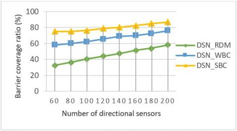
4.1 Impact of the number of directional sensors
In the first scenario, we change the number of deployed directional sensors from 60 to 200 in order to calculate the barrier coverage ratio achieved using the proposed approaches and the random deployment model. The comparative results are presented in Figure 9. We can observe that the barrier coverage ratio for all three approaches is gradually increasing. The reason is that as long as more directional sensors are deployed, more sensors will be selected to cover the barrier. However, the proposed model DSN_SBC performs better since the coverage is improved using mobile directional sensors with an optimization of their orientation which gives us the possibility to cover more points in the barrier vicinity. This improvement is explained by the fact that by moving the directional sensors closer to the barrier, we reduce the distances between the sensors and the points to be monitored, which increases the probability of capturing events and obtaining a better barrier coverage. The rapprochement of the sensors also creates new intersections between their fields of view (overlaps). This means that several sensors can now monitor the same area, which enhances the detection and tracking capacity of events.
Figure 9. Barrier coverage ratio with various number of directional sensors
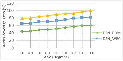
Figure 10. Barrier coverage ratio with various AoV
4.2 Impact of the angle of view (AoV)
In this subsection, we evaluate the impact of the AoV on the performance of the proposed approaches. For this experiment, we fixed the number of directional sensors to 120, the DoV to 10m and the AoV varied from 30° to 110°. It can be observed from Figure 10 that the barrier coverage ratio increases with larger AoV, because a directional sensor can cover more points when its AoV increases. Therefore, the barrier region covered by a directional sensor is directly proportional to its AoV. The DSN_WBC approach performs better than DSN_RDM model, the reason is that the novel configuration of directional sensors’ orientation with a larger AoV allows to cover the barrier vicinity as much as possible. We can see clearly from Figure 10 that the barrier coverage ratio tends to reach a maximum with an AoV=110° using the DSN_SBC model. In this case, we can generate more overlapped sensor’s AoV because all sensors will be in the vicinity of the barrier. Furthermore, redundant sensors give us the possibility to prolong the network lifetime and then to achieve a high coverage ratio.
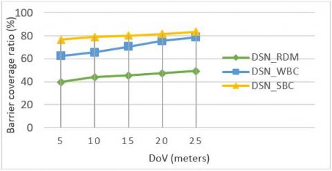
4.3 Impact of the depth of view (DoV)
In this simulation scenario, we evaluated the effect of changing the DoV on the performance of the proposed approaches. In this experiment, we fixed the AoV to 30°, the number of directional sensors to 120 and the DoV varied from 5 to 25m. As illustrated in Figure 11, a high coverage ratio can be obtained using the proposed approaches DSN_WBC and DSN_SBC compared with DSN_RDM with a larger value of DoV. It can also be observed that the value of DoV has an impact on the behavior of DSN_WBC. The reason is that when the DoV increases, we can achieve a satisfactory barrier coverage ratio by selecting a significant number of appropriate directional sensors to cover the barrier. Furthermore, a better simulation result is obtained with the DSN_SBC model because with a larger value of DoV, mobile directional sensors have the possibility to complete barrier coverage with the stationary directional sensors without having to change position.
Figure 11. Barrier coverage ratio with various DoV
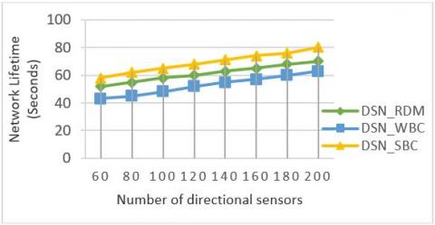
4.4 Network lifetime with various number of directional sensors
We have also studied the comparative performances of the network lifetime of the weak barrier DSN_WBC and strong barrier DSN_SBC approaches with the original model DSN_RDM by varying the number of deployed directional sensors. As depicted in Figure 12, the network lifetime increases almost linearly when the number of directional sensors increases because the coverage can be ensured by more sensors. We can also observe from this figure that DSN_RDM has a longer network lifetime compared with DSN_WBC, because the DSN_RDM algorithm does not cause directional sensors to change direction, so it can save more energy. The graphs also show that DSN_SBC performs better than DSN_RDM and DSN_WBC. The reason is that we generate more overlapping areas when a large number of directional sensors are oriented in the same direction. In this case, we have possibility to keep some redundant directional sensors in an inactive state because their AoV are already covered by their neighbors. Furthermore, with this approach we can recover the energy consumed for the movement of the mobile directional sensors. This strategy allows us to save energy and therefore to prolong the network lifetime.
Figure 12. Network lifetime with various number of directional sensors
In this paper, we investigated the barrier coverage problem in DSNs, which is suitable for many surveillance applications, especially border protection, by exploring stationary and mobile directional sensors. We proposed two distributed algorithms to improve the barrier coverage ratio using hybrid DSNs. The first algorithm optimizes directional sensors’ orientation to improve coverage and to achieve a weak barrier coverage. In the second one, we developed a solution to reach a strong barrier coverage by exploiting mobile directional sensors. This strategy allows us to generate more redundant sensors and therefore to minimize the number of active directional sensors. The simulation results demonstrate that this second approach outperforms the first algorithm and the random deployment model in terms of barrier coverage enhancement and energy consumption and show the benefits of using mobile directional sensors.
In terms of future work, firstly, we intend to make additional extensions to the proposed model to reduce energy consumption. Secondly, we will extend the performance evaluation by including the comparison of additional existing approaches. Finally, we plan to develop a testbed and to implement the proposed algorithms in a real environment.
[1] Cheng, C.F., Hsu, C.C. (2021). The deterministic sensor deployment problem for barrier coverage in WSNS with irregular shape areas. IEEE Sensors Journal, 22(3): 2899-2911. https://doi.org/10.1109/JSEN.2021.3137626
[2] Guvensan, M.A., Yavuz, A.G. (2011). On coverage issues in directional sensor networks: A survey. Ad Hoc Networks, 9(7): 1238-1255. https://doi.org/10.1016/j.adhoc.2011.02.003
[3] Costa, D.G., Guedes, L.A. (2010). The coverage problem in video-based wireless sensor networks: A survey. Sensors, 10(9): 8215-8247. https://doi.org/10.3390/s100908215
[4] Qarehkhani, A., Golsorkhtabaramiri, M., Mohamadi, H., Yadollahzadeh Tabari, M. (2021). Solving target coverage problem in directional sensor networks with ability to adjust sensing range using continuous learning automata. Journal of Intelligent & Fuzzy Systems, 41(6): 6831-6844. https://doi.org/10.3233/JIFS-210759
[5] Chen, G., Xiong, Y., She, J., Wu, M., Galkowski, K. (2020). Optimization of the directional sensor networks with rotatable sensors for target-barrier coverage. IEEE Sensors Journal, 21(6): 8276-8288. https://doi.org/10.1109/JSEN.2020.3045138
[6] Zarei, Z., Bag‐Mohammadi, M. (2021). Coverage improvement using Voronoi diagrams in directional sensor networks. IET Wireless Sensor Systems, 11(3): 111-119. https://doi.org/10.1049/wss2.12015
[7] Bendimerad, N., Kechar, B. (2018). Coverage enhancement with occlusion avoidance in networked rotational video sensors for post-disaster management. International Journal of Information and Communication Technology, 12(3-4): 319-344. https://doi.org/10.1504/IJICT.2018.090417
[8] Bendimerad, N., Boumedjout, A., Bot, B. (2022). Distributed algorithm for area monitoring in directional sensor networks. In International Conference on Computing and Information Technology. Cham: Springer International Publishing, pp. 329-340. http://doi.org/10.1007/978-3-031-25344-7_29
[9] Tao, D., Wu, T. (2015). A survey on barrier coverage problem in directional sensor network. IEEE Sensors Journal, 15(2): 876-885. http://doi.org/10.1109/JSEN.2014.2310180
[10] Kumar, S., Lai, T.H., Arora, A. (2005). Barrier coverage with wireless sensors. In Proceedings of the 11th Annual International Conference on Mobile Computing and Networking, pp. 284-298. https://doi.org/10.1145/1080829.1080859
[11] Liu, B., Dousse, O., Wang, J., Saipulla, A. (2008). Strong barrier coverage of wireless sensor networks. In Proceedings of the 9th ACM International Symposium on Mobile ad Hoc Networking and Computing, pp. 411-420. https://doi.org/10.1145/1374618.1374673
[12] Chen, A., Kumar, S., Lai, T. (2010). Local barrier coverage in wireless sensor networks. IEEE Transactions on Mobile Computing, 9(4): 491-504. https://doi.org/10.1109/TMC.2009.147
[13] Chen, A., Li, Z., Lai, T.H., Liu, C. (2011). One-way barrier coverage with wireless sensors. In 2011 Proceedings IEEE INFOCOM, Shanghai, China, pp. 626-630. https://doi.org/10.1109/INFCOM.2011.5935241
[14] Fan, F., Ji, Q., Wu, G., Wang, M., Ye, X., Mei, Q. (2018). Dynamic barrier coverage in a wireless sensor network for smart grids. Sensors, 19(1): 41. https://doi.org/10.3390/s19010041
[15] Li, Q., Liu, N. (2022). Coverage optimization algorithm based on control nodes position in wireless sensor networks. International Journal of Communication Systems, 35(5): e4599. https://doi.org/10.1002/dac.4599
[16] Chakraborty, M., Rout, M. (2021). Optimal barrier coverage in randomly scattered wireless sensor networks. In 2021 12th International Conference on Computing Communication and Networking Technologies (ICCCNT), Kharagpur, India, pp. 1-6. http://doi.org/10.1109/ICCCNT51525.2021.9579537
[17] Cheng, C.F., Hsu, C.C., Pan, M.S., Srivastava, G., Lin, J.C.W. (2022). A cluster-based barrier construction algorithm in mobile wireless sensor networks. Physical Communication, 54: 101839. https://doi.org/10.1016/j.phycom.2022.101839
[18] Yao, P., Guo, L., Li, P., Lin, J. (2023). Optimal algorithm for min-max line barrier coverage with mobile sensors on 2-dimensional plane. Computer Networks, 228: 109717. https://doi.org/10.1016/j.comnet.2023.109717
[19] Khanjary, M., Sabaei, M., Meybodi, M.R. (2018). Barrier coverage in adjustable-orientation directional sensor networks: A learning automata approach. Computers & Electrical Engineering, 72: 859-876. http://doi.org/10.1016/j.compeleceng.2018.01.009
[20] Binh, N.T.M., Binh, H.T.T., Le Loi, V., Nghia, V.T., San, D.L., Thang, C.M. (2019). An efficient approximate algorithm for achieving (k−!) barrier coverage in camera wireless sensor networks. In Artificial Intelligence and Machine Learning for Multi-Domain Operations Applications. SPIE, 11006: 387-399. http://doi.org/10.1117/12.2519272
[21] Chen, J., Wang, B., Liu, W., Yang, L., Deng, X. (2017). Rotating directional sensors to mend barrier gaps in a line-based deployed directional sensor network. IEEE Systems Journal, 11(2): 1027-1038. http://doi.org/10.1109/JSYST.2014.2327793
[22] Cheng, C.F., Hsu, C.C. (2021). The deterministic sensor deployment problem for barrier coverage in WSN with irregular shape areas. IEEE Sensors Journal, 22(3): 2899-2911. https://doi.org/10.1109/JSEN.2021.3137626
[23] Binh, N.T.M., Binh, H.T.T., Ngoc, N.H., Anh, M.D.Q., Phuong, N.K. (2021). Maximizing lifetime of heterogeneous wireless turnable camera sensor networks ensuring strong barrier coverage. Journal of Computer Science and Cybernetics, 37(1): 57-70. http://doi.org/10.15625/1813-9663/37/1/15858
[24] Hong, Y., Luo, C., Li, D., Chen, Z., Wang, X. (2022). Lifetime-Maximized strong barrier coverage of 3D camera sensor networks. Wireless Communications & Mobile Computing (Online), 2022. https://doi.org/10.1155/2022/2659901
[25] Wang, Z., Liao, J., Cao, Q., Qi, H., Wang, Z. (2013). Achieving k-barrier coverage in hybrid directional sensor networks. IEEE Transactions on Mobile Computing, 13(7): 1443-1455. http://doi.org/10.1109/TMC.2013.118
[26] Liu, X.L., Yang, B., Chen, G.L. (2015). Barrier coverage in mobile camera sensor networks with grid-based deployment. arXiv Preprint arXiv, 1503.05352. https://doi.org/10.48550/arXiv.1503.05352
[27] Zhao, L., Bai, G., Shen, H., Tang, Z. (2018). Strong barrier coverage of directional sensor networks with mobile sensors. International Journal of Distributed Sensor Networks, 14(2): 1550147718761582. http://doi.org/10.1177/1550147718761582
[28] Liu, X.L., Yang, B., Chen, G.L. (2019). Full-view barrier coverage in mobile camera sensor networks. Wireless Networks, 25: 4773-4784. https://doi.org/10.1007/s11276-018-1764-6
[29] OMNeT++Discrete Event Simulator, http://www.omnetpp.org/, accessed on Sep. 15, 2023.