Long-Term Forecasting of Crop Water Requirement with BP-RVM Algorithm for Food Security and Harvest Risk Reduction

Land is important for people whose lives depend on the agricultural sector. A developing country always makes strategies to improve food security for its people. Therefore, some areas are designated as national food estates [1]. Muthayya et al. [2] mentioned that Indonesia is one of several countries with the largest rice production in the world. Together with China, India Bangladesh, Vietnam, Myanmar, Thailand, the Philippines, Japan, Pakistan, Cambodia, the Republic of Korea, Nepal, and Sri Lanka, Asian countries account for 90% of the world's total rice production [3].

Policies on climate change are crucial to maintain the stability of food security because climate change affects an area’s water availability as well as environmental, social, and agricultural systems. Therefore, Riptanti et al. [4] stated that information on climate change and water availability is required to increase crop productivity, especially in drylands. The climate change in question is closely related to the annual trend of hydro-climatological data. Therefore, hydro-climatological data is very important in planning planting schedules, which are part of a good cropping pattern. A proper planting schedule must follow the interval of water availability based on climate change throughout the year. The positive impact is to improve national food security.

One of the purposes of hydro-climatological forecasting is to predict climate change and determine farmers’ cropping pattern [5]. Hydro-climatological data include rainfall (mm), temperature (℃), humidity (%), sunshine duration (hours), and wind speed (knots). From time to time, these data change and shift, especially rainfall. It affects the timing and pattern of planting, which farmers should change accordingly. The process of determining planting patterns cannot be separated from the optimization of irrigation systems, land area, agricultural production, and other indicators in agriculture. There are various studies on irrigation system optimization for determining irrigation water requirement [6-14]. The implementation of irrigation system is limited to wetlands, which have reservoirs used to meet water requirements. Therefore, cropping pattern planning should be applicable in both wetlands and drylands, which can only be planted with rainfall overflow.

In addition, on average, farmers realize that using local technology causes low crop productivity as well as low income. These problems generally occur due to the lack of institutional support from the government for farmers' activities [15]. Meanwhile, food production index has a significant and positive impact on poverty reduction [16, 17].

Modeling or forecasting of hydro-climatological data has been widely applied in the fields of economics, planning, construction, transportation, and agriculture. Bathia and Rana [18] used linear programming to determine the allocation and combination of crops in each growing season. Villagrán [19] made a greenhouse simulation for fruit and vegetable production by taking into account wind speed and temperature data. Ramli et al. [20] used linear regression with a log transformation to predict rainfall data, rainfall, total of rainy days, temperature, humidity, duration of irradiation, and wind speed for 29 years to forecast climate change. The model found was only able to predict with an R-square value of 24.61% and RMSE value of 57.676. Therefore, they recommended that the forecasting of hydro-climatological data should use non-linear methods for better data pattern recognition. The utilization of linear methods is sometimes only able to be trained on a relatively small amount of data. Therefore, a method that is capable of training a large amount of data and is more complex is needed.

A forecasting method with non-linear functions is artificial neural network backpropagation (ANN-BP). ANN have been widely used for hydro-climatological data forecasting and the most popular data predicted is rainfall [21-24]. This is done because rainfall has an important role to determine weather and climate changes. ANN-BP algorithm with two hidden layers was used by Irawan et al. [25] to predict hydro-climatological data for determining crop water requirement and planning planting patterns. Architecture with two hidden layers was also used by Syaharuddin et al. [26] to forecast inflation data with the training function is trainrp and the activation function of each layer is logsig. The process of increasing the number of hidden layers in the ANN-BP architecture will certainly make it easier for the network to recognize data patterns. Furthermore, the experimental results of Vera et al. [27], using the activation function and the training function, found that the results of training data using a backpropagation architecture with three hidden layers are better than two hidden layers. The MSE and MAPE values are 0.0382 and 0.1954, respectively, when using two hidden layers, while when using three hidden layers, the MSE and MAPE values are 0.0375 and 0.1936, respectively.

The forecasted hydro-climatological data can be used to calculate evaporation, evapotranspiration (potential and actual), effective rainfall, and crop water requirement. Generally, researchers use the Penman method (1948) to determine the potential evapotranspiration value if the station recording hydro-climatological data provides complete data. However, at some locations or actual data recording stations, the data is sometimes unavailable or limited. This means that one or more of the five hydro-climatological data is incomplete or the data recording unit is not daily. Thus, scientists developed other methods such as Thomthwaite (1948), Makkink (1957), Blaney-Criddle (1959), Turc (1961), Hamon (1961), Rohwer (1962), Jensen-Haise (1963), Penman-Monteith (1965), Priestley-Taylor (1972), Hargreaves (1975), Doorenbos-Pruitt (1977), Kharrufa (1985), Linacre (1977), and Abtew (1996) [28-32]. These methods have been redeveloped according to Food and Agriculture Organization (FAO) standards; among them are Penman-Monteith, Blaney-Criddle, Turc, Jensen-Haise, Jensen, Priestley-Taylor, and Hargreaves [33-38].

Researches continuously experiment with the methods that have been modified in order to determine a reliable method to obtain evapotranspiration values. Chiew et al. [39] analyzed climate characteristics in 16 Australian locations and found that the FAO24 radiation, FAO24 Blaney-Criddle, and Penman-Monteith gave similar monthly ET, estimates. This result is reinforced by the results of research [40-43], which showed that the Blaney-Criddle method gave good calculation results of evapotranspiration values, which was close to the results found using the FAO Penman-Monteith method as a basic method. This finding is an important basis for researchers in determining evapotranspiration and crop water requirement when hydro-climatological data are incomplete at a location.

The results of of hydro-climatological data forecasting and calculation of evapotranspiration and crop water requirement need to be integrated due to the multi-year nature of the cropping pattern planning procedure. It has still been done by many other researchers, where forecasting is only done for one current year. Meanwhile, cropping pattern planning is multi-year. Hence, long-term forecasting must be carried out to obtain hydro-climatological data of the coming year. In addition, many researchers only focus on rice as the staple food although in one heterogeneous land, other crops such as CGPRT crops (coarse grains, pulses, roots and tubers), horticultural crops, and even tobacco must also be planted. Therefore, the purpose of this research is to explain the implementation of artificial neural network backpropagation and relevance vector machine (BP-RVM) for long-term forecasting of hydro-climatological data. Furthermore, we calculate evapotranspiration values, effective rainfall, and irrigation water requirements, and crop water requirements during the cropping process based on the forecasting results. The results of this research are expected to be useful in planning optimal cropping patterns and serve as a basis for the government in devising policies on agriculture.

Generally, the growing requirements of each crop depends on climatic indicators such as rainfall (mm/month), temperature (℃), and humidity (%). The growing requirements of each crop are different (Table 1), thus affecting the crop planting schedule for each season. Therefore, these needs must be taken into account in planning a good cropping pattern, especially water requirement.

Rainfall is the main indicator for all crops. In planning cropping patterns, hydro-climatological data must be considered, especially in the data forecasting process. Initially, forecasting data is used to determine the evapotranspiration value and water requirement of each crop during the pre-planting, planting, and harvesting (including post-planting) processes. Evapotranspiration is the evaporation of the surface of a field overgrown with plants, which is a combination of evaporation and transpiration stages [45]. Meanwhile, crop water requirements are generally determined by evapotranspiration and effective rainfall [46, 47]. The actual crop evapotranspiration value (mm/day) can be determined using Eq. (3):

$E t_c=K_c \cdot E t_o$     (3)

with K_c indicating crop coefficient (Table 2) [48] and indicating potential evapotranspiration (mm/day) [49]. Crop coefficients are characteristics of crops used to predict evapotranspiration values and have different values according to the length of planting of food crops. Meanwhile, potential evapotranspiration is a value that describes the need for the environment, a set of vegetation, or an agricultural area to evapotranspire which is determined by several factors, such as sunlight intensity, wind speed, leaf area, air temperature, and air pressure.

Table 1. Growing conditions and crop harvest time

Table 2. K_c value according to the food and agriculture organization (FAO)

Table 2 shows that each crop has a different coefficient value (K_c), which affects the evaporation and evapotranspiration values of each crop [50, 51]. $E t_o$ value can be determined with various methods according to the types of available data, such as rainfall, temperature, wind speed, humidity, and sunshine duration. In this study, the authors used the FAO24 Blaney-Criddle method as shown in Eq. (4) [36]:

$E t_o=a+b p(0.46 T+8.13)(1+0.0001 E)$     (4)

with T is temperature (℃); p is empirical coefficients based on latitude (⁰) (see Figure 1); E is elevation (m) [52]; a and b are calibrated constants obtained using Eq. (5) and Eq. (6):

$a=0.0043\left(R H_{\text {min }}\right)-\left(\frac{n}{N}\right)-1.41$      (5)

$\begin{gathered}b=0.88165+0.857596\left(\frac{n}{N}\right)- \\ 0.00454\left(\left(R H_{\min }\right)+0.093803\left(U_d\right)\right)- \\ 0.00405\left(\left(R H_{\min }\right)\left(\frac{n}{N}\right)-0.00087\left(R H_{\min }\right)\left(U_d\right)\right)\end{gathered}$     (6)

with RH_min as the lowest daily relative humidity (%); n/N as the average ratio of actual to possible sunshine duration (%); and U_d as wind speed. Furthermore, the p-value in Eq. (4), shown in Figure 1, was taken from the position of Kediri station, which is close to a latitude of 10⁰ (see Figure 2).

1.png

Figure 1. P-value based on blaney-criddle method

$E t_o$  value can be used to calculate water requirement for rice production or irrigation water requirement (IR) with Eq. (7):

$I R=\frac{M e^k}{e^k-1}$      (7)

with e=2.7182; $M=1.1 E t_o+3 ; k=\frac{3 M}{25}$.

Furthermore, the effective rainfall (R_eff) for rice (Eq. (8)) is different from that for CGPRT crops (Eq. (9)).

$R_{e f f}=0.7 \frac{R_{80}}{10}$         (8)

$R_{e f f}=0.7 \frac{R_{50}}{10}$      (9)

$R_{80}$ and $R_{50}$  are the mainstay rainfall determined from all data used as input for making forecasting using the BP-RVM architecture. Furthermore, Eq. (3) and Eqs. (8)-(9) were used to determine crop water requirement with Eqs. (10)-(11).

$N F R=E t_c+P-R_{e f f}+W L R,($ for rice $)$      (10)

$N F R=E t_c+P-R_{e f f},($ for CGPRT crops, horticulture, etc)     (11)

P is the location that shows soil infiltration; in this study, the P-value was 3 mm/day. WLR is the turnover of subsoil water carried out twice a month (semi-monthly according to the fertilization schedule); each was 50mm (3.3 mm/day for 15 days).

5.1 Hydro-climatological data forecasting results

Based on Figure 2, there are three rainfall stations, namely Gunung Sari Station, Lembar Station, and Kediri Station. The forecasting results from these three stations are averaged before calculating the effective rainfall value. We utilized average statistics because cropping pattern planning is global for the West Lombok district. This has an impact on government calculations in determining the amount of food crop seed and fertilizer supplies before distribution. The results of the average rainfall calculation will not significantly affect the calculation of effective rainfall and other parameters. While the temperature, wind speed, humidity, and sunshine duration data still use data from Kediri station. This is due to the climatology data recording tool only being available at Kediri station. The architecture in Figure 3 is used for data in long-term forecasting using Eq. (1), meaning that 2012-2021 data is used for 2022 data forecasting, then 2012-2021 data and 2022 forecasting results are used for 2023 data forecasting. The forecasting results are shown in Table 3.

Table 3. Descriptive results of hydro-climatological data forecast

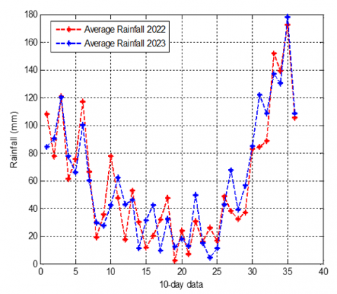
Table 3 indicates that the number of epochs generated is between 27 and 52. When predicting rainfall data, the smallest number of epochs was found from data obtained from Gunung Sari station, while the highest was found from data taken from Lembar station. Furthermore, the highest average of rainfall was found in the Kediri station area. Geographically, this station is located in a flat area, whereas Gunung Sari and Lembar areas which are in mountainous areas. In addition, the MSE value of each data could be found. A higher value indicates that the data have high fluctuations and vice versa. For example, temperature data that is relatively static has an average MSE value of 0.31. The forecasting results also showed that the maximum average rainfall in 2022 and 2023 would be 172.53 mm and 178.33 mm, respectively. Overall, taking into account the MAPE value based on Lewis' classification [55], the average forecasting results fall into the “good forecasting” category. The distribution of forecasting data based on long-term forecasting is shown in Figures 4-8.

4.png

Figure 4. Forecasting data of rainfall

5.png

Figure 5. Forecasting data of temperature

6.png

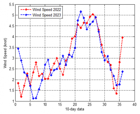
Figure 6. Forecasting data of wind speed

7.png

Figure 7. Forecasting data of humidity

8.png

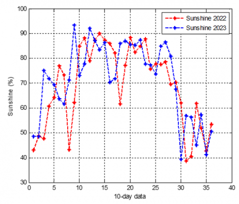
Figure 8. Forecasting data of sunshine duration

Generally, Figures 4-8 demonstrate that the trend of each data is relatively stable. The forecasting data of the year 2023 does not appear to have different fluctuations from the forecasting data in 2022. Rainfall forecasting data in Figure 4 show that rainfall in 2023 tends to increase compared to 2022 with a peak occurring in December 2022 of 417.01 mm and starting to decline at the end of February 2023.

Furthermore, the temperature forecasting data in Figure 5 show that there would be an increase in temperature in September-October every year, reaching more than 28⁰C as the rainy season would begin in this period. Wind speed forecasting data in Figure 6 show that the maximum wind speed would occur in July-August, reaching 5 knots. The speed would increase again in early January, reaching more than 4 knots. The humidity forecasting data in Figure 7 show an increase at the beginning, middle, and end of the year with an average of 84.28%. Finally, the forecasting data of sunshine duration in Figure 8 show that there would be an increase at the end of March and decrease at the end of August. Humidity would be between 79% and 89%. Humidity is strongly influenced by temperature, wind speed, rainfall, sunshine duration, and vegetation density [56, 57]. This means that high rainfall will increase the density of plant vegetation, which can increase humidity in an area with high vegetation.

The amount of water, temperature, and humidity suitable for each crop shown in Table 4 were calculated based on the criteria in Table 1 and the results of data forecasting. These values can be used as a reference to determine the appropriate planting season (PS) for each crop.

Table 4. Rainfall suitability for crops

Based on the rainfall forecasting in Figure 4, rainfall in 2022 would start to increase in October 2022, meaning that the planting season (PS-1) could begin that month. Therefore, Table 4 shows that almost all crops are suitable to be planted between late October and February, except peanut, cassava, sweet potato, tobacco, and watermelon. Generally, these crops could be planted in the dry season (PS-2 and PS-3). Table 4 also shows that there would be very little rainfall in August, so it would not be suitable to plant any of the crops that month.

5.2 Effective rainfall and irrigation water requirements

The forecasting results of hydro-climatological data were used to calculate the potential evapotranspiration value (Eq. (4)), water requirement for rice production or irrigation water requirement (Eq. (7)), and effective rainfall (Eqs. (8)-(9)). The calculation results are shown in Figure 9.

9.png

Figure 9. Rainfall conditions and water requirements for rice production

Irrigation water requirement is the amount of water needed to meet the needs for crop evaporation, water loss, water requirements by taking into account the amount of water provided by nature through rainfall and beneath the ground. Figure 9 illustrates that the ratio of rainfall to water requirement for rice production is normal. The average irrigation water requirement throughout 2022-2023 would be 12.36mm. It would be met by rainfall except in July 2022, June 2023, and August 2023 because the dry season (PS-3) with very low or zero rainfall intensity would take place in these months.

10.png

Figure 10. Et_o value and effective rainfall

Based on Figure 10, it can be seen that the potential evapotranspiration value throughout 2022-2023 would be between 2.82mm/day and 4.38 mm/day with an average of 3.6 mm/day and a maximum of 4.38mm/day at the end of September 2023. Meanwhile, effective rainfall for both rice and CGPRT crops would be very high in the December-January-February (DJF) period with a maximum value of 8.4mm/day for rice and 11.06mm/day for CGPRT crops. In the March-April-May (MAM) period, the value would decrease since this period occurs in the dry season and the beginning of PS-2.

5.3 Actual evapotranspiration and crop water requirements

The actual crop evapotranspiration value (Eq. (3)) and crop water requirement (Eqs. (10)-(11)) were determined according to the planting schedule in a year. Figure 4 shows that the rainfall data at the end of October 2022 would reach more than 50mm. This means that the planting season (PS-1) for rice and crops that meet the growing requirements could begin. Thus, the suitable planting season should begin between late October 2022 and early October 2023. Hence, in the interval of the growing season, the value of Et_c and NFR can be determined according to Figure 11 and Figure 12.

11.png

Figure 11. Average value of Et_c

12.png

Figure 12. Average value of NFR

The evapotranspiration value of rice was higher than that of CGPRT crops, tobacco, and horticultural crops. The maximum Et_c value of rice was 4.5 mm/day, the minimum value was 2.99 mm/day, with an average of 3.79 mm/day. Figure 11 also presents the high evapotranspiration value of tobacco. This high value was obtained due to the relatively long harvest time of tobacco with an average coefficient (K_c) of 0.86. This value was higher than the coefficient of CGPRT crops and horticultural crops (see Table 2). Finally, the evapotranspiration values of crops and horticulture were almost the same with an average of 2.20 mm/day (CGPRT crops) and 2.19 mm/day (horticultural crops). This occurred because the morphology and coefficient of CGPRT and horticultural crops are almost the same, namely 0.76 and 0.75 respectively.

Crop water requirements are dominantly influenced by the actual evapotranspiration value of and the effective rainfall for each crop [58, 59]. Figure 12 shows that rice has the highest water requirement compared to CGPRT crops, tobacco, and horticultural crops. Meanwhile, the crops suitable to be planted in the dry season (PS-2 and PS-3) statistically have the same water requirements.