Malathi Mani* | Senthil Kumar Angamuthu
© 2022 IIETA. This article is published by IIETA and is licensed under the CC BY 4.0 license (http://creativecommons.org/licenses/by/4.0/).
OPEN ACCESS
Wireless sensor network (WSN) becomes a popular research area, finds useful in the process of surveillance and archiving of sensitive data. WSN includes numerous compact sized, low powered, battery powered sensor nodes, which finds applicability in several areas of border surveillance, healthcare, objective tracking, environmental observance, etc. Therefore, critical importance raises several security issues. Owing to the open-access of physical media, the WSN is susceptible to jamming attacks, which interferes with the radio frequency employed by the networking nodes. The jamming attack detection can be considered as an NP-hard problem and optimization algorithms can be employed to resolve it. This paper presents a new jamming attack detection and defence scheme using quasi oppositional spider monkey optimization (SMO) algorithm, named QOSMO. The SMO algorithm is stimulated from the intelligent foraging behavior of spider monkeys that replicate the fission–fusion social structure. However, the perturbation rate is one of the important parameters of the SMO algorithm, which disturbs the convergence rate. To improve the convergence rate, quasi oppositional SMO (QOSMO) algorithm is employed. The presented QOSMO algorithm detects the jamming attack using different metrics namely detection rate, end to end (ETE) delay, throughput, and packet loss to determine the jamming attacks in WSN. The QOSMO model is implemented in the MATLAB tool. The experimental results portrayed that the QOSMO model has outperformed the other methods by defeating the jamming attacks and maintaining the overall network efficiency.
jamming attack, WSN, spider monkey algorithm, convergence rate, quasi oppositional based learning
Wireless sensor networks (WSN) is one of the well-known and extensively applied method in various applications of military surveillance, hospitals, and many other emergency spots such as meteorological climate observations, security domain, factory automation, etc. WSN is composed of tiny and cost-effective sensor nodes without any infrastructure. The major responsibility of any sensor node is to sense, compute, forward, and receive the details from a specific region before sending it to a Base Station (BS) or sink. Typically, WSN is embedded with numerous sensor nodes which are classified on the basis of the structure or topology and the type of atmosphere it is placed. WSNs are divided according to the placement of sensor nodes [1]. Most of the nodes have similar potential whereas other nodes have different capabilities that depend upon the structure. There are 3 classes of WSN namely, Flat-based (tree), Cluster-based, and Hierarchical. Also, the deployment of sensor nodes in a WSN is clustered into five categories such as underground, Terrestrial, Underwater, Multi-media, and Mobile WSNs [2].
Mostly, the sensor nodes are placed in regions like remote, harsh, inaccessible, and unattended places which are simplified by the resource limitations such as minimum energy, restricted memory, least bandwidth as well as shortest transmission radius. At the same time, it is coupled with the vulnerability of wireless medium (open and shared) and has resulted in malicious sensor nodes for various security intrusions like Denial of Service (DoS). For instance, DoS attack on DYN which is considered as Domain Name System (DNS) provider in the last decades. The DYN DDoS attack is orchestrated using a botnet named Mirai malware that has affected numerous terminal nodes and the Internet of Things (IoT) devices [3]. Researchers have examined the distributed form of DoS which is assumed as a tedious attack and the magnitude ranged from 1.2 Tbps. Jamming attacks are referred to as DoS attack in which the adversary forwards a high-range signal to interrupt communication. Jamming occurs unexpectedly in a wireless medium under constrains like Noise, Interference, and Collision [4], but, a jamming attack in WSN is a conscious attempt for physical signal transmission at the time of communication. The key objective of the DoS attack is to send the suspicious signals to sensor nodes and communication channels to degrade the resources like battery duration, bandwidth, and memory to eliminate the transmitted sensor data to reach the target where long-term availability is affected.
Followed by, a jamming attack in WSN is dangerous as the special hardware or software is not required. It is performed by passive listening to a wireless medium for broadcasting the identical frequency band as the broadcasting signal. The jamming attack is considered by maximum power efficiency, minimum prediction probability, as well as anti-jamming resistance [5]. In WSN, a physical layer and Medium access control (MAC) layer are the typical destinations of DoS jamming attacks. Figure 1 shows the development of a jamming attack in WSN.
Figure 1. Scenario of Jamming attack in cluster based WSN
In order to predict the jamming attacks in WSN, some of the recently developed models are implanted with sensor nodes. Such technologies apply data attained from prior regarding the communication behavior at the time of normal and jammed state which has been monitored under the application of indicators and metrics accomplished from diverse layers. The samples of these metrics are obtained from signal strength at a physical layer and Packet Delivery Ratio (PDR) at the functional layer. Moreover, the newly utilized approaches have presented a cross-layer structure for collecting jamming attack indicators and enhance the prediction of jamming attacks.
The contribution of the paper is given as follows. This paper presents a new jamming attack detection and defense scheme using quasi oppositional spider monkey optimization (SMO) algorithm, named QOSMO. The QOMSO incorporates the traditional concepts of the SMO algorithm and quasi oppositional based learning (QOBL) mechanism. Initially, The SMO algorithm is based on the fascinating nature of spider monkeys that replicate the fission-fusion social structure. Since the perturbation rate an essential parameter of the SMO algorithm, it interrupts the convergence rate. For improving the convergence rate, the QOSMO algorithm is employed to detect jamming attacks under various aspects.
In WSN, securities of wireless devices as well as communication structure are assumed to be challenging problems due to the dynamicity and unknown behavior. This work recommends different types of methods for resolving the problems related to WSN security or privacy. Researchers have projected an effective approach for resolving the issues involved in the secure communication structure. The network threatening factor aims in hijacking network security for network traffic observation, failure in wireless nodes, jam network traffic, interrupt the complete system. Therefore, the awful attack over the jamming attack interrupts the complete communication system. Some of the recommended methods for eliminating jamming attacks are defined under. In multi-joint relay as well as jammer chosen approach was projected by Zhang et al. [6]. It has employed a secure decoding unit for accessing the input signal before and after transmission. Moreover, it has employed an artificial broadcast signal for diverting the intruder, before attacking the confidential information.
Feng et al. [7] employed the random Markov chain model for developing a multi-agent system structure for preventing strategic cyber-attacks in wireless systems. Tang et al. [8] recommended a triggering principle for jamming attack prediction like DoS in mobile robots. It validates the presented method in an operational atmosphere for tracking mobile robots for the prediction of jamming attacks. Sharma et al. [9] established a lightweight performance rule specification approach for identifying the cyber-physical attacks in WSNs. Therefore, the projected scheme applies the communication data obtained from placed sensors for identifying the jamming attacks. The key objective of the newly presented approach is to find the suspicious sensor node in a system using transmission behavior. Also, an automated verification technique has been applied frequently to verify the operational network for predicting jamming attacks. The intrusion detection system (IDS) is applied in past decades for network security from physical attacks. Therefore, using classical as well as ordinary IDS to WSNs is highly challenging because of the minimum resources and dynamic nature.
The fault examination technique for Unmanned Surface Vehicle System (USVS) has been presented by Ma et al. [10]. This technology is operated in 3 phases like Event triggering; Event base switching and Piecewise function to validate the legitimacy of network traffic as well as transmission media. Initially, the event relied on triggering models are highly significant for predicting and preventing the jamming attacks. Also, the USVS approach employs data like communication delay and interruption of communication for the prediction of jamming attacks. Ge et al. [11] applied the review of previous models used in the detection and elimination of jamming attacks in WSN. The New Resilient Based Security (NRBS) framework for preventing jamming attacks as presented by Al-Shammari et al. [12]. In NRBS model, the developers have applied data like information delivery and energy utilization of typical nodes to predict jamming attacks in WSNs.
Lu et al. [13] introduced a channel training technology for identifying the covert pilot spoofing attacks in WSN. This mechanism is well-equipped and efficient while predicting eavesdropping and routing intrusions of WSN. Therefore, the intrusion classification is performed according to the threshold value of a transmission channel, but it is not so efficient in a poor transmission state. Thus, a channel training technology is produced only in a general WSNs communication atmosphere; however it is ineffective in physical disasters like weather, fidelity, and attenuation, and the effectiveness ratio of the presented approach is reduced. Then, non-orthogonal multiple access (NOMA) as well as Hybrid Automatic Repeat Request (HARQ) methodologies, were implied by Xiang et al. [14]. The unification of NOMA and HARQ has been employed in the newly presented technology for enhancing the security of WSN.
The LAM-CIoT lightweight authorization approaches were projected by Wazid et al. [15]. This mechanism is employed in a cloud-based IoT structure to prove the security of data gathered from sensors placed in a remote position concerning one-way cryptographic hash function authentication. Wazid et al. [16] presented the secure key management as well as the user confirmation approach named SAKA-FC in case of fog computing environment and deploy the secure communication system. The combination of one-way cryptographic hash function and bitwise-OR (XOR) has been applied in this model to validate the legitimacy of applied devices in a system.
2.1 Limitation of the literature
Generally, WSN includes the sensors which are limited in resources and it has a dynamic behavior. Thus, the effective application of these systems enhances the ability and scalability. WSN is comprised of massive wireless nodes, which are malicious in various types of attacks as sensor nodes are placed in unattended or harsh regions. The jamming attack is dreadful as it damages the communication process of WSN. Hence, the newly developed study has recommended diverse models to reduce the jamming attacks on the WSNs platform. Unexpectedly, some of the disadvantages of WSN are:
Figure 2 shows the working principle of the QOSMO algorithm for detecting jamming attacks in WSN. The figure shows that the nodes in WSN are randomly utilized in the target area. Then, the nodes are initialized and collect information about their neighbors. Afterward, the BS executes the QOSMO algorithm for detecting the existence of a jamming attack in the network.
Figure 2. Block diagram of the proposed model
3.1 SMO algorithm
SMO is defined as meta-heuristic approach evolved from intelligent foraging nature of SM. The foraging hierarchy of SM depends upon the fission-fusion social structure. A feature of SM relies on the social organization of a group in which a female leader rules the team and makes decisions. The dominant one of a group is termed as a global leader whereas the leaders of tiny sets are called local leaders. Using the SMO model, food scarcity is one of the negative sign in foraging nature. SMO is evolved from the Swarm Intelligence (SI) related method where a small group is comprised of the least number of monkeys. Thus, while computing a fission development with a minimum count of monkeys, also the fusion mechanism should be computed. In the SMO method, SM implies a capable solution. In general, Spider monkey resides in tropical rain forests of Central and South America and exists in Mexico [17]. It is one of the smart animals among New World monkeys. It is named as spider monkeys as it looks like spiders if it is suspended by their tails. Spider monkey always tries to reside in a set named as the parent group. According to the food scarcity or accessibility, it divides themselves as lonely or in groups. The communication between the groups which depends upon the gestures, locations, and whooping. Group composition is defined as a dynamic feature in this architecture:
A social communication as well as the performance of spider monkeys are known from the given objectives:
1. Spider monkeys often reside in groups with 50 members.
2. The individuals in a community forage in tiny groups in diverse directions and it shares the foraging nature in the night at the habitat.
3. The dominant female spider monkey selects a foraging route.
4. When a leader does not identify enough food; afterward it is clustered into smaller groups that are foraged separately.
5. Individuals of the group are not considered in the nearby position due to the mutual tolerance between once another.
Figure 3. Foraging behavior of spider monkey
Spider monkeys distribute the observations under the application of positions and gestures. In longer distances, they communicate with one another by specific sounds like whooping or chattering. Every monkey is composed of discernible sound by another group member to find the monkey. The foraging behaviors of spider monkeys are depicted in Figure 3.
SMO is comprised of 6 phases namely, Local Leader phase (LLP), Global Leader phase (GLP), Local Leader Learning Phase, Global Leader Learning phase, Local Leader Decision phase, and Global Leader Decision phase.
Initialization:
At first, SMO produces a uniformly distributed swarm of $N$ SMs, in which $S M_i$ denotes a $i^{\text {th }} \mathrm{SM}$ in a swarm. All $S M_i$ is initiated in the following:
$S M_{i j}=S M_{\min j}+U\left(0_t 1\right) \times\left(S M_{\max j}-S M_{\min j}\right)$ (1)
where, $S M_{\min j}$ and $S M_{\max j}$ means the maximum and minimum bounds of a search space in jth dimension as well as U(0,1) denotes a uniformly distributed random value from (0,1).
Local leader phase (LLP):
This is one of the reputed phases of the SMO method. In this approach, all SMs is probable to upgrade them. The change in the position of SM depends upon the local leader and experience of local group members. The fitness score of all SM is determined in a novel position and when the fitness is maximum than the former one, and it is upgraded. The position update function is expressed as:
$SMnew _{i j}=S M_{i j}+U(0,1) \times\left(L L_{k j}-S M_{i j}\right)$$+U(-1,1) \times\left(S M_{r j}-S M_{i j}\right)$ (2)
where, SMij indicates the jth dimension of ith SM, LLkj implies a jth dimension of the local leader of kth group and SMrj denotes jth dimension of an arbitrarily chosen SM from kth group where r≠i and U(-1, 1) is a uniformly distributed value within (-1, 1). In this approach, it is evident from the Eq. (2) that the SM is ready to upgrade the position, and it is attracted to the local leader at the time of retaining self-confidence. Hence, the final component guides result in conflicts, especially in the search process, and assists in maintaining the stochastic behavior of the method in order that premature death is ignored. The entire position updating mechanism is defined in Algorithm 1. Here, pr shows a perturbation rate for the present solution, and values emerges from [0.1, 0.8].
|
Algorithm 1: Position update process in LLP |
|
for all $S M_i \in k^{T h}$ group do for all $j \in\{1, \ldots, D\} d o$ if $U(0,1) \geq p r$ then SMnew $_{i j}=S M_{i j}+U(0,1) \times\left(L L_{k j}-S M_{i j}\right)+$$U(-1,1) \times\left(S M_{r j}-S M_{i j}\right)$ else $SMnew _{i j}=S M_{i j}$ end if end for end for |
Global leader phase (GLP):
Once the LLP phase is completed, then GLP mechanism is initialized. In this approach, solutions are upgraded according to the selection probability named as fitness function (FF). Hence, the objective function fi is a fitness fiti is determined using Eq. (3).
$fitnessfunction=fit_i= \begin{cases}\frac{1}{1+f_i}, & \text { if } f_i \geq 0 \\ 1+a b s\left(f_i\right), & \text { if } f_i<0\end{cases}$ (3)
The selection probability probi is evaluated on the basis of roulette wheel selection. When a fiti is fitness of ith SM and probability of being elected from a GLP have been measured with the help of given functions:
$prob_i=\frac{\text { fitness }_i}{\sum_{i=1}^N \text { fitness }_i}$ or $prob_i=0.9 \times \frac{f i t_i}{\text { max }_{-} f i t}+0.1$
In order to upgrade the position, SM applies the experience of a global leader where neighboring SM and its efficiency. The position upgrading function of this stage is computed using the given function:
$S M n e w_{i j}=S M_{i j}+U(0,1) \times\left(G L_j-S M_{i j}\right)$$+U(-1,1) \times\left(S M_{r j}-S M_{i j}\right)$ (4)
where, GLj signifies a position of the global leader in jth dimension. The position update function is classified as 3 components in which the initial component implies perseverance of a parent SM, followed by, the second element depicts the attraction of a parent SM to a global leader, and the final element is employed for retaining the stochastic nature of this approach.
From this expression, the second component is mainly employed for enhancing the exploitation of previously recognized search space whereas a third component guides in removing the premature death in search space. The entire searching model of this phase is described in Algorithm 2 as shown below:
|
Algorithm 2: Position update process in GLP |
|
Count =0; When count 0< group size do for all members $S M_i \in$ group do if $U(0,1)< prob_i$ then count = count +1 Randomly choose $j \in\{1, \ldots, D\}$ Randomly choose $S M_r \in$ group s.t. $r \neq i$ $SMnew _{i j}=S M_{i j}+U(0,1) \times\left(G L_j-S M_{i j}\right)+$$U(-1,1) \times\left(S M_{r j}-S M_{i j}\right)$ end if end for end while |
From Algorithm 2, it is evident that the possibility of solution enhancement depends upon the probi. Hence, solutions with maximum fitness have a higher possibility when compared with minimum fitness solutions. Furthermore, a greedy selection scheme has been utilized for upgrading the solutions where the maximized SM is attained and named as an optimal fit solution.
Global leader learning phase:
Here, the method identifies an optimized solution from a total swarm. Therefore, the predicted SM is assumed as a global leader. Moreover, the location of a global leader is verified and when they are not upgraded then it is termed as Global Limit Count (GLC), which is enhanced by 1, else it can be 0 The GLC is validated for global leaders and related to Global Leader Limit (GLL).
Local leader learning phase:
In this phase, the place of a local leader is maximized using a greedy selection mechanism. When a leader does not upgrade the position, afterward a counter is associated with a local leader named Local Limit Count (LLC) that is improved by 1; else 0. It can be used in all groups to identify local leaders. Likewise, LLC is a counter which is enhanced until reaching a fixed threshold referred to as Local Leader Limit (LLL).
Local leader decision phase:
Before invoking this phase, LL and GL have to be discovered. When the LL is not reformed into a specific verge, named as LLL then every member of a group upgrades the positions with the help of random initialization using Eq. (5). It is employed with a probability pr so-called as perturbation rate.
$SMnew_{i j}=S M_{i j}+U(0,1) \times\left(G L_j-S M_{i j}\right)$$+U(0,1) \times\left(S M_{r j}-L L_{k j}\right)$ (5)
From this expression, it is clear that solutions emerged from this group is evolved from previous LL as it is released and solutions are attracted to the GL for changing the traditional searching directions and locations. Moreover, it depends upon the pr, and the dimension of solutions is initiated randomly from the existing position. Then, LLL is a parameter used in validating the LL whether it is trapped in local minima and measured as D×N, where D refers to a dimension and N implies the overall count of SM. When LLC is higher than LLL after that LLC is 0 and SM is again repeated for enhancing the search space. The procedure of the local leader decision phase is explained in Algorithm 3.
|
Algorithm 3: Local Leader Decision Phase (LLD) |
|
If LLC >LLL then LLC =0 for all $j \in\{1, \ldots, D\}$ do if $U(0,1) \geq p r$ then $SMnew_{i j}=S M_{\min j}+U(0,1) \times\left(S M_{\max j}-S M_{\min j}\right)$ else $SMnew_{i j}=S M_{i j}+U(0,1) \times\left(G L_j-S M_{i j}\right)+$$U(0,1) \times\left(S M_{r j}-L L_{k j}\right)$ end if end for end if |
Global leader decision phase:
As same as previous phase, when the GL is not reformed within a specific verge termed as GLL, then a GL portions a swarm into tiny groups or combine the groups as a single unit. In this segment, GLL is one of the parameters that validates whether the premature convergence exits, and differs from N/2 to 2×N. When GLC is maximum than GLL then, GLC becomes 0 and count of groups is related to maximum groups. When the previous count of groups is minimum than the existing count of groups then, GL has divided again into groups; else it integrates a single or parent group. Hence, the fission-fusion process is defined in Algorithm 4.
|
Algorithm 4: Global Leader Decision Phase (GLD): |
|
if GLC > GLL then GLC =0 if No. of groups <MG then Classify the swarms into groups else Integrate the groups to develop a single group end if upgrade LLP end if |
3.2 Quasi oppositional based learning
As the perturbation rate is a vital parameter of the SMO algorithm, it disturbs the convergence rate. For improving the convergence rate, the QOSMO algorithm is employed to detect jamming attacks.
Opposition‐based learning (OBL) is the purpose of boosting candidate solutions by means of the recent population and the inverse population simultaneously. Evolutionary optimization models are invoked with few populations and attempts to enhance the solution and model efficiency. The searching operation is terminated while the pre-determined criterion is attained. It is initialized only when the prior knowledge is unavailable regarding the optimal solution. This process can also be enhanced by making the closer optimal solution as a fitter solution by validating the inverse solution. Then, a fitter has been selected as the primary solution. Based on the possibility, the guess is away from the solution when compared with the inverse guess. Hence, this operation is initiated with nearby guesses. Followed by a similar technique has been used for the initial solution and every solution present in the recent population.
Quasi-OBL was developed by Rao and Rai [18] for maximizing the candidate solution under the concern of recent population and corresponding QOBL simultaneously. The above-mentioned process is extended by initializing nearby function which is considered a better solution at the time of validating QO solution. This is performed for the sake of selecting a fitter as a major solution. It is invoked using adjacent guesses. However, same method is not employed for initial solution and it is also utilized for the solution present in all populations. By doing this, it has ensured that quasi-opposite number is closer when compared to a random value of a solution. Moreover, it has assured that quasi‐opposite number is always nearby opposite value of a solution. The fundamental strategy of QOBL approach has been employed in population initialization as well as in generation jumping.
Opposite and quasi‐opposite numbers
Consider that x is a real value among [lb, ub], the opposite value (xo) and the quasi‐opposite value (xqo) are illustrated as:
$x_0=l b+l u-x$ (6)
and
$x_{q o}=\operatorname{rand}\left[\left(\frac{l b+l u}{2}\right),(l b+l u-x)\right]$
Likewise, the description is expanded to maximum dimensions as defined in the following:
Opposite and quasi‐opposite points
Assume that X=(x1, x2, …, xn) is a point in n‐dimensional space in which xi∈[lbi, ubi] as well as i∈1, 2, …, n. The opposite point Xo=(x01, x02, …, xon) is depicted as given Eq. (7):
$x_{o i}=l b_i+u b_i-x_i$ (7)
The quasi‐opposite point Xqo=(xqo1, xqo2, …, xqon) is explained as provided in Eq. (8):
$x_{q o i}=\operatorname{rand}\left[\left(\frac{l b_i+l u_i}{2}\right),\left(l b_i+l u_i-x_i\right)\right]$ (8)
Using the description of QO point, the optimization mechanism is illustrated in the following section.
Quasi‐opposition based optimization
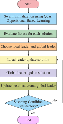
Assume that X=(x1, x2, … , xn) is a point in n‐dimensional space named as a candidate solution. Let f=(∙) denotes a FF applied for measuring the candidate’s fitness. Based on the description of quasi‐opposite point, Xqo=(xqo1, xqo2, …, xqon) is referred to as quasi‐opposite of X=(x1, x2, …, xn). Then, (Xqo)<f(X) is a point X which is replaced with $X_{q o}$; else, this process is followed by X. Therefore, a point and the corresponding quasi-opposite point are determined concurrently to identify the fittest solution. Figure 4 illustrates the flowchart of the QOSMO model.
Figure 4. Flowchart of QOSMO algorithm
3.3 QOSMO algorithm based Jamming Attack Detection
The BS executes the QOSMO algorithm for detecting the existence of a jamming attack in the network. The QOSMO algorithm derives a FF using distance, energy, signal to noise ratio (SNR), and packet loss. The derived FF helps to define the occurrence of jamming attacks.
Proposed fitness function$=$ Dist $*$ Energy $* S N R *$ Packet Loss (9)
The first parameter ‘distance’ is determined at the first stage when the nodes in WSN are placed in a 2D plane using Euclidean distance, as shown below:
$D_{a b}=\sqrt{\left(X_a-X_b\right)^2+\left(Y_a-Y_b\right)^2}$ (10)
where, a and b are the two nodes representing the source and destination.
In case of the presence of jamming attack, the alternate path is considered by increasing the hop count. Since the hop count gets increased, the existence of jamming attack can be detected. Next, the second parameter energy defines the total amount of residual energy available at the node. The third parameter SNR defines the level of the desired signal to the level of background noise. SNR is attained by determining the ratio of the received signal power to the received noise power at the node. It is an important measure to detect jamming attacks in the physical layer since jamming resulted in a decrease in SNR value. Finally, the packet loss signifies the count of packets gets missed at the time of communication. The packet loss gets increased with the presence of jamming attack [19]. The proposed QOSMO algorithm determines the jamming attack using the above mentioned FF.
This section explains the experimental validation of the QOSMO algorithm. The results are investigated in terms of four different measures namely detection rate, throughput, packet loss, and ETE delay. The parameter setting of the QOSMO algorithm is provided in Table 1.
Table 1. Parameter setting
|
Parameter |
Value |
|
Area |
100*100 m2 |
|
Simulation tool |
MATLAB |
|
Node count |
200 |
|
Attack type |
Jamming attack |
|
Bandwidth |
10Mbps |
|
Channel Delay |
2 µs |
|
Network topology |
Random |
|
Packet size |
64kbps |
4.1 Analysis of Jamming attack detection rate
Table 2 and Figure 5 illustrates the jamming attack detection rate of the QOSMO algorithm with existing methods under varying number of jamming attacks launched. From the figure, it is seen that the DSCC algorithm has exhibited poor results by attaining minimum jamming attack detection rate. At the same time, the EBTC algorithm has tried to exhibit slightly higher jamming attack detection. Followed by, the BRIoT and ACCS algorithms have exhibited moderate performance by attaining near optimal jamming attack detection rate. But the proposed QOSMO algorithm has showcased superior results by offering maximum jamming attack detection rate. For instance, under the existence of 100 jamming attacks launched, the presented QOSMO model has reached a maximum detection rate of 100 whereas the BRIoT, EBTC, DSCC, and ACCS have showcased minimum detection rate of 89.87, 85.49, 83.31, and 96.44. Similarly, under the existence of 500 jamming attacks launched, the presented QOSMO model has attained to a maximum detection rate of 499 while the BRIoT, EBTC, DSCC, and ACCS have exhibited minimum detection rate of 446.75, 429.23, 407.34, and 468.64.
Figure 5. Jamming attacks detection rate analysis of QOSMO model
Likewise, under the existence of 1000 jamming attacks launched, the presented QOSMO model has achieved a maximum detection rate of 950 but the BRIoT, EBTC, DSCC, and ACCS have outperformed minimum detection rate of 891.27, 858.36, 832.09, and 928.42.
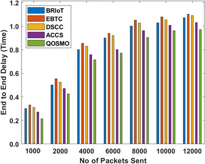
4.2 Analysis of ETE delay
Table 3 and Figure 6 depict the ETE delay of the QOSMO model with existing methods under varying number of packets sent. From the figure, it is seen that the EBTC method has showcased the worst results by attaining maximum ETE delay. At the same time, the DSCC technique has tried to exhibit a somewhat lower ETE delay. Followed by, the BRIoT and ACCS algorithms have demonstrated moderate performance by reaching near optimal ETE delay. But the proposed QOSMO model has outperformed superior results by offering minimum ETE delay. For instance, under the existence of 1000 packets sent, the proposed QOSMO model has attained a minimum ETE delay of 0.2142ms whereas the BRIoT, EBTC, DSCC, and ACCS have showcased maximum ETE delay of 0.30ms, 0.33ms, 0.31ms, and 0.27ms.
Figure 6. End to end delay analysis of QOSMO model
4.3 Analysis of throughput
Table 4 and Figure 7 showcase the throughput statistical analysis of QOSMO method with existing methods under varying number of packets sent. From the figure, it is seen that the DSCC algorithm has demonstrated poor outcomes by attaining minimum throughput statistical analysis. At the same time, the EBTC algorithm has tried to exhibit slightly higher throughput statistical analysis. Followed by, the BRIoT and ACCS algorithms have exhibited moderate performance by reaching near-optimal throughput statistical analysis. But the proposed QOSMO algorithm has showcased superior results by offering maximum throughput statistical analysis. For instance, under the existence of 5000 throughput statistical analysis, the presented QOSMO model has reached a maximum throughput of 4385.1 whereas the BRIoT, EBTC, DSCC, and ACCS have showcased minimum throughput of 3992.5, 3948.04, 3948.04, and 4036.1.
Table 2. Jamming attacks detection rate of QOSMO model
|
Total No. Jamming attacks launched |
BRIoT |
EBTC |
DSCC |
ACCS |
QOSMO |
|
100 |
89.87863 |
85.49978 |
83.31036 |
96.4469 |
100.2666 |
|
200 |
179.645 |
166.5085 |
168.6979 |
186.2133 |
200.1403 |
|
300 |
271.6008 |
256.2749 |
249.7066 |
282.548 |
310.152 |
|
400 |
361.3672 |
339.473 |
328.5259 |
376.6932 |
400.7989 |
|
500 |
446.7548 |
429.2394 |
407.3451 |
468.649 |
499.8165 |
|
600 |
538.7106 |
510.2481 |
492.7327 |
564.9837 |
595.1212 |
|
700 |
613.151 |
597.825 |
578.1202 |
650.3712 |
689.6584 |
|
800 |
691.9703 |
665.6972 |
648.1818 |
727.0011 |
765.3712 |
|
900 |
792.6838 |
768.6001 |
744.5165 |
823.3357 |
870.0011 |
|
1000 |
891.2079 |
858.3665 |
832.0934 |
928.4281 |
950.9654 |
Table 3. End to end delay of QOSMO model
|
No of Packets Sent |
BRIoT |
EBTC |
DSCC |
ACCS |
QOSMO |
|
1000 |
0.302556 |
0.33067 |
0.310223 |
0.271885 |
0.2142 |
|
2000 |
0.501913 |
0.553031 |
0.524916 |
0.471243 |
0.425982 |
|
4000 |
0.80095 |
0.854623 |
0.829065 |
0.7575 |
0.7143 |
|
6000 |
0.900629 |
0.938967 |
0.921076 |
0.80095 |
0.77126 |
|
8000 |
1.000308 |
1.051425 |
1.025866 |
0.96197 |
0.90453 |
|
10000 |
1.028422 |
1.07954 |
1.053981 |
1.007975 |
0.96191 |
|
12000 |
1.071872 |
1.102542 |
1.089763 |
1.030978 |
0.97124 |
Table 4. Throughput analysis of QOSMO model
|
No. of Packets Sent |
BRIoT |
EBTC |
DSCC |
ACCS |
QOSMO |
|
5000 |
3992.507 |
3948.042 |
3948.042 |
4036.972 |
4385.106 |
|
10000 |
7905.402 |
7860.937 |
7860.937 |
7905.402 |
8056.204 |
|
15000 |
13729.37 |
13773.83 |
13729.37 |
13862.76 |
13900.83 |
|
20000 |
18686.73 |
18642.26 |
18731.19 |
18731.19 |
18812.04 |
|
25000 |
22377.3 |
22288.37 |
22510.69 |
22688.55 |
22750.37 |
Table 5. Number of packet loss of QOSMO method
|
No. of Packets Sent |
BRIoT |
EBTC |
DSCC |
ACCS |
QOSMO |
|
5000 |
1007.493 |
1051.958 |
1051.958 |
963.0281 |
614.894 |
|
10000 |
2094.598 |
2139.063 |
2139.063 |
2094.598 |
1943.796 |
|
15000 |
1270.633 |
1226.169 |
1270.633 |
1137.239 |
1099.17 |
|
20000 |
1313.274 |
1357.739 |
1268.809 |
1268.809 |
1187.958 |
|
25000 |
2622.703 |
2711.632 |
2489.309 |
2311.45 |
2249.63 |
4.4 Analysis of packet loss
Table 5 and Figure 8 show the packet loss of the QOSMO model with existing methods under varying number of packets sent. From the figure, it is seen that the EBTC method has showcased worst results by attaining maximum packet loss. Simultaneously, the DSCC technique has tried to exhibit somewhat lower packet loss. Afterward, the BRIoT and ACCS algorithms have exhibited moderate performance by reaching near-optimal packet loss. But the proposed QOSMO model has outperformed superior results by offering minimum packet loss.
Figure 7. Throughput analysis of QOSMO model
Figure 8. Packet loss analysis of QOSMO model
For instance, under the existence of 5000 packets sent, the proposed QOSMO model has attained a minimum packet loss of 614.89 whereas the BRIoT, EBTC, DSCC, and ACCS have outperformed maximum packet loss of 1007.49, 1051.95, 1051.95, and 963.02. By looking into the experimental results, it is ensured that the QOSMO algorithm has showcased effective performance over the compared methods.
This paper has presented a new jamming attack detection and defence scheme using QOSMO algorithm. Initially, the nodes in WSN are randomly deployed in the target area. Then, the nodes are initialized and collect information about their neighbors. Afterward, the BS executes the QOSMO algorithm to detect the existence of a jamming attack in the network. The QOSMO algorithm derives a FF using distance, energy, SNR, and packet loss. The proposed QOSMO method detects the jamming attacks proficiently over the compared methods. The experimental outcome stated that the QOSMO algorithm has outperformed the other methods in a significant way. The proposed model shown its superiority by attaining effective results in terms of packet loss, ETE delay, throughput, and detection rate. In future, the detection performance can be increased by the use of deep learning approaches. We also plan to extend the model for anomaly detection in IoT and cloud environment.
[1] Osanaiye, O.A., Alfa, A.S., Hancke, G.P. (2018). Denial of service defence for resource availability in wireless sensor networks. IEEE Access, 6: 6975-7004. https://doi.org/10.1109/ACCESS.2018.2793841
[2] Yick, J., Mukherjee, B., Ghosal, D. (2008). Wireless sensor network survey. Computer Networks, 52(12): 2292-2330. https://doi.org/10.1016/j.comnet.2008.04.002
[3] Bharathi, L., Chandrabose, S. (2022). Machine learning-based malware software detection based on adaptive gradient support vector regression. International Journal of Safety and Security Engineering, 12(1): 39-45. https://doi.org/10.18280/ijsse.120105
[4] Li, M., Koutsopoulos, I., Poovendran, R. (2010). Optimal jamming attack strategies and network defense policies in wireless sensor networks. IEEE Transactions on Mobile Computing, 9(8): 1119-1133. https://doi.org/10.1109/TMC.2010.75
[5] Pelechrinis, K., Iliofotou, M., Krishnamurthy, S.V. (2010). Denial of service attacks in wireless networks: The case of jammers. IEEE Communications Surveys & Tutorials, 13(2): 245-257. https://doi.org/10.1109/SURV.2011.041110.00022
[6] Zhang, G., Gao, Y., Luo, H., Sha, N., Guo, M., Xu, K. (2019). Security performance analysis of joint multi-relay and jammer selection for physical-layer security under Nakagami-m fading channel. IEICE Transactions on Fundamentals of Electronics, Communications and Computer Sciences, 102(12): 2015-2020. https://doi.org/10.1587/transfun.E102.A.2015
[7] Feng, Z., Wen, G., Hu, G. (2016). Distributed secure coordinated control for multiagent systems under strategic attacks. IEEE Transactions on Cybernetics, 47(5): 1273-1284. https://doi.org/10.1109/TCYB.2016.2544062
[8] Tang, Y., Zhang, D., Ho, D.W., Yang, W., Wang, B. (2018). Event-based tracking control of mobile robot with denial-of-service attacks. IEEE Transactions on Systems, Man, and Cybernetics: Systems, 50(9): 3300-3310. https://doi.org/10.1109/TSMC.2018.2875793
[9] Sharma, V., You, I., Yim, K., Chen, R., Cho, J.H. (2019). BRIoT: Behavior rule specification-based misbehavior detection for IoT-embedded cyber-physical systems. IEEE Access, 7: 118556-118580. https://doi.org/10.1109/ACCESS.2019.2917135
[10] Ma, Y., Nie, Z., Hu, S., Li, Z., Malekian, R., Sotelo, M. (2020). Fault detection filter and controller co-design for unmanned surface vehicles under DoS attacks. IEEE Transactions on Intelligent Transportation Systems, 22(3): 1422-1434. https://doi.org/10.1109/TITS.2020.2970472
[11] Ge, X., Han, Q.L., Zhang, X.M., Ding, L., Yang, F. (2019). Distributed event-triggered estimation over sensor networks: A survey. IEEE Transactions on Cybernetics, 50(3): 1306-1320. https://doi.org/10.1109/TCYB.2019.2917179
[12] Al-Shammari, H.Q., Lawey, A.Q., El-Gorashi, T.E., Elmirghani, J.M. (2020). Resilient service embedding in IoT networks. IEEE Access, 8: 123571-123584. https://doi.org/10.1109/ACCESS.2020.3005936
[13] Lu, X., Yang, W., Cai, Y., Guan, X. (2019). Proactive eavesdropping via covert pilot spoofing attack in multi-antenna systems. IEEE Access, 7: 151295-151306. https://doi.org/10.1109/ACCESS.2019.2948078
[14] Xiang, Z., Yang, W., Pan, G., Cai, Y., Song, Y., Zou, Y. (2019). Secure transmission in HARQ-assisted non-orthogonal multiple access networks. IEEE Transactions on Information Forensics and Security, 15: 2171-2182. https://doi.org/10.1109/TIFS.2019.2955792
[15] Wazid, M., Das, A.K., Bhat, V., Vasilakos, A.V. (2020). LAM-CIoT: Lightweight authentication mechanism in cloud-based IoT environment. Journal of Network and Computer Applications, 150: 102496. https://doi.org/10.1016/j.jnca.2019.102496
[16] Wazid, M., Das, A.K., Kumar, N., Vasilakos, A.V. (2019). Design of secure key management and user authentication scheme for fog computing services. Future Generation Computer Systems, 91: 475-492. https://doi.org/10.1016/j.future.2018.09.017
[17] Bansal, J.C., Sharma, H., Jadon, S.S., Clerc, M. (2014). Spider monkey optimization algorithm for numerical optimization. Memetic Computing, 6(1): 31-47. https://doi.org/10.1007/s12293-013-0128-0
[18] Rao, R.V., Rai, D.P. (2017). Optimization of submerged arc welding process parameters using quasi-oppositional based Jaya algorithm. Journal of Mechanical Science and Technology, 31(5): 2513-2522. https://doi.org/10.1007/s12206-017-0449-x
[19] Sasikala, E., Rengarajan, N. (2015). An intelligent technique to detect jamming attack in wireless sensor networks (WSNs). International Journal of Fuzzy Systems, 17(1): 76-83. https://doi.org/10.1007/s40815-015-0009-4