Anuja Jana Naik* | Gopalakrishna Madigondanahalli Thimmaiah
© 2021 IIETA. This article is published by IIETA and is licensed under the CC BY 4.0 license (http://creativecommons.org/licenses/by/4.0/).
OPEN ACCESS
Detection of anomalies in crowded videos has become an eminent field of research in the community of computer vision. Variation in scene normalcy obtained by training labeled and unlabelled data is identified as Anomaly by diverse traditional approaches. There is no hardcore isolation among anomalous and non-anomalous events; it can mislead the learning process. This paper plans to develop an efficient model for anomaly detection in crowd videos. The video frames are generated for accomplishing that, and feature extraction is adopted. The feature extraction methods like Histogram of Oriented Gradients (HOG) and Local Gradient Pattern (LGP) are used. Further, the meta-heuristic training-based Self Organized Map (SOM) is used for detection and localization. The training of SOM is enhanced by the Fruit Fly Optimization Algorithm (FOA). Moreover, the flow of objects and their directions are determined for localizing the anomaly objects in the detected videos. Finally, comparing the state-of-the-art techniques shows that the proposed model outperforms most competing models on the standard video surveillance dataset.
Anomaly detection and localization, histogram of oriented gradients, local gradient pattern, self-organized map, fruit fly optimization algorithm
Surveillance has emerged to a remarkable level in modern technology such that it can be utilized to ensure the safety and security of the public [1]. CCTV cameras have been broadly utilized to monitor and record circumstances for offering evidence to the surveillance scheme. The eminence of surveillance videos has been improved by 9.3% in the year 2019. CCTV cameras are regularly utilized in forensic procedures for post-video analysis of earlier events [2]. It means the feed of CCTV is required to be monitored manually with a human operator when any unusual events occur suddenly in the scene. An anomalous or abnormal event is a maneuver that emerges mistrusts by conflicting the common activities [3]. Some realistic circumstances such as uncrowded, crowded, indoor and outdoor may lead to main challenges like causing more damage, death, injury, a terrorist attack, a robbery, and an area invasion [4]. Thus, it is necessary to develop an anomaly detection and localization model for an effective surveillance system.
Some of the major limitations needed to be considered for efficient modeling of automated anomaly detection and localization are the size of the dataset, time consumption, complex scene, and localization of object [3, 5]. The crowded scene includes various objects with occlusions and complex clutter, leading to an increase in interest. [6]. It is solved by adapting two major techniques, such as (a) traditional-based methods and (b) deep learning-based methods, which mainly focus on anomaly detection in crowds. The anomaly events are detected using hand-crafted features like motion and appearance features in the traditional-based methods. The accuracy of this approach is based on the appearances of objects and motion cues. It can also be performed by extracting features and object tracking [7]. However, in deep learning-based models, complex scenarios are handled using a learnable system of nonlinear transformation [8].
The significant contribution of this proposed model is given below.
To develop a new anomaly detection and localization model for crowded videos using objects' flow, directions, and FOA-based SOM.
To extract the features from the input patterns using HOG and LGP and the dimensionality reduction approach called PCA.
To detect the anomaly in video features by using optimized SOM, in which the optimization of the weight of SOM is done by a new algorithm called FOA.
To achieve better convergence by considering the objective function with the maximization of precision for the proposed detection and localization of the anomalies in videos.
To evaluate the performance of the proposed model by comparing it with conventional models on the standard UCSD dataset.
The remaining sections of this proposed architectural view of anomaly detection and localization model in the video are explained in Section 3. Section 4 explains the optimized SOM or video anomaly detection. Section 5 discusses the results of the proposed model. Section 6 concludes this paper.
Identifying and locating anomalies in the video is a major complex errand in the computer vision domain. Existing approaches consider it an outlier detection issue that measures the variation between the tested and normal samples. Diverse models are proposed in the literature that has different features and challenges. Many deep learning networks are employed to extract high-level representations from the scene's sub-areas [2]. Different approaches have been proposed for anomaly detection in literature, such as the Convolutional 3D(C3D) network, Principal Component Analysis Network (PCANet), spatial-temporal Convolutional Neural Network, auto-encoder, restricted Boltzmann machine (RBMs), deep-anomaly, deep-cascade, etc. Various researchers have used the benefits of Generative Adversarial Network (GAN) for detection in normal frames [6]. The test frame is considered abnormal when there is a mismatch in the prediction and discovery of the test frame or the recognition of the test frame, which is represented as fake using the discriminator [9]. The network training requires additional manual involvement, and the representations of learning have confirmed the efficiency of deep learning networks in detecting and localizing anomaly tasks.
A novel robust PCA-based foreground localization method was developed by Wang et al. [10]. This method has merged the standard 2D texture descriptor called LGP with the OF for developing a Uniform Local Gradient Pattern Based Optical Flow (ULGP-OF) descriptor developed to describe the statistics of the motion in the local region using the foreground localization method. The ULGP-OF and Spatially Localized Histogram of Optical Flow (SL-HOF) methods have established better discriminative performance when compared to any traditional video descriptors. A method called One-Class Extreme Learning Machine (OCELM) [10] uses the features of normal video events and thus improves the testing and training speed and attains better outcomes than conventional approaches. This approach cannot be applied to the hierarchical Extreme Learning Machine (ELM)-autoencoder.
A new unsupervised approach using GAN and Edge Wrapping (EW) named Deep Spatiotemporal Translation Network (DSTN) was developed by Ganokratanaa et al. [11]. In this method, the temporal features are generated using dense OF from the frames of normal events. A new fusion of background removal using indigenous and background removal frames is introduced based on appearance and motion features. Similarly, the performance is improved in the pixel-level assessment by developing the EW for minimizing the noise and suppressing the unrelated edges of anomalous entities. The results of this model have established better performance in terms of time complexity, pixel-level assessment, and frame-level assessment for abnormality detection of object and localization tasks.
The problem with this method is that it cannot use an object translation system through a clustering technique for complex scenes. Gaussian Mixture Fully Convolutional-Variational Autoencoder (GMFC-VAE) [12] attains better detection performance and learns anomalies even from the normal samples. Though, it is not appropriate to use Reinforcement Learning (RL). Cheng et al. [13] presented a hierarchical structure to detect local and global anomalies using a GPR and hierarchical feature representation that was completely robust and non-parametric to the training of noisy data, thus supporting the sparse features. It attains a better detection rate and achieves better competence performance.
On the other hand, it cannot handle the temporal association. Xu et al. [14] proposed a model which extracted spatial-temporal features using Shape Convolutional Layers (SCL) and Motion Convolutional Layers (MCL) without splitting or resizing the frames. The adaptiveness of this model was enhanced by Adaptive Intra-Frame Classification Network (AICN), where an intra-frame classifier and Adaptive Region Pooling Layer (ARPL) were used. ARPL and the intra-frame classifier offer better classification results and a faster detection speed. However, there is a need to adopt kernel learning. These challenges are considered while developing a video anomaly detection and localization model using a deep learning approach.
3.1 Developed model
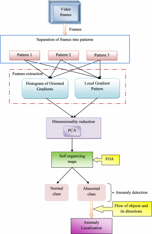
The detection of anomalies in videos plays a major role in the surveillance sector. Recent works classically suffer from the limitations in detecting objects and localization because of the complex and crowded scenes. An important major challenge is the scarcity of samples containing abnormal events for training. It leads to the inadequacy of data and thus escalates the complexity of developing better classifiers. Additionally, training for all possible abnormal events is not required due to the unpredictable nature of real-world incidents. Thus, the current work focuses on unsupervised deeplearning-based methodologies to overcome the limitations mentioned above. The performance of object localization is also another limitation of pixel-level anomaly detection. This pixel-level evaluation is more difficult when compared to the frame-level evaluation due to the complex nature of anomaly localization. Therefore, there is a need to develop an efficient anomaly detection and localization model using unsupervised learning. The proposed anomaly detection and localization model is given in Figure 1.
The proposed model considers the input as videos from the UCSD standard dataset. The frames in the video are separated into three patterns for further processing based on some criteria. Pattern 1 represents the consecutive frames; pattern 2 represents the frames selected after skipping one frame after one, and pattern 3 represents the frames selected after skipping five frames after one. These attained three patterns are subjected to the feature extraction process for each video. The most significant features are extracted using two approaches like HOG and LGP. These are efficient approaches for object recognition. The attained features are given to the dimensionality reduction technique called PCA for obtaining the significant features. The anomaly detection is performed using SOM, in which the training weight is optimized using the FOA. The optimized SOM is employed to cluster frames into two classes like normal class and abnormal class. Hence, the proposed FOA-SOM helps to accomplish the anomaly detection of video, and further, the anomaly localization is performed by the flow of objects and their directions. As a contribution, the proposed automated anomaly detection and localization model intends to maximize the precision of the newly developed model. Consider, Zij is the video frames, in which ij=1,2,…. FD and FD denote the total number of videos in the dataset. The ijth video consists of a GF number of frames.
Figure 1. Automated Anomaly detection and localization model
3.2 Dataset description
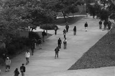
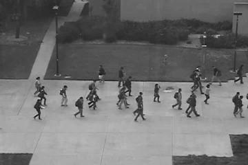
UCSD dataset is an anomaly detection dataset collected using a stationary camera. It includes videos of a crowded pedestrian walkway with two subsets called Ped1 and Ped2, denoted as dataset 1 and dataset 2, respectively. It is recorded at two diverse scenes through a camera. The first dataset includes 14 abnormal and 16 normal video clips with a size of 320×240 pixels. In the UCSD Ped2 dataset, the length of every video clip is between 150 to 200 frames. Here, the normal events include pedestrians on the pathways, and the abnormal events consist of skaters, small cars, bikes, and pedestrians in the surrounding pathways. The clip length of UCSD Ped1 is specified as 200 frames, whereas Ped1 is given among 150-200 frames.
3.3 Feature extraction
It is the initial stage in the proposed model where the features of the input video frames based on three different patterns are extracted using the approaches like HOG and LGP. The details of the feature extraction methods are discussed below.
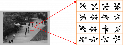
Figure 2. HOG feature extraction for proposed model
HOG [15]: It is an efficient approach for the recognition of objects. These features are computed with captivating orientation histograms of edge intensity in a local region with a size of 16×16 pixels. The total count of HOG features extracted is 128, which is represented in Figure 2.
The gradients and orientations of the edge are obtained using Sobel filters from the local region. The computation of orientation(y,z) and gradient magnitude g(y,z) is done using Sobel filters based on y and z directional gradients dy(y,z) and dz(y,z), which are formulated in Eq. (1) and Eq. (2).
$\varphi(y, z)=\left\{\begin{aligned} {\tan ^{-1}\left(\frac{d z(y, z)}{d y(y, z)}\right)-\pi} &\quad {if d y(y, z)<0 \& d z(y, z)>0} \\ {\tan ^{-1}\left(\frac{d z(y, z)}{d y(y, z)}\right)+\pi} &\quad { if d y(y, z)<0\& d z(y, z)>0} \\ {\tan ^{-1}\left(\frac{d z(y, z)}{d y(y, z)}\right)} &\quad otherwise \end{aligned}\right.$ (1)
$g\left( y,z \right)=\sqrt{dy{{\left( y,z \right)}^{2}}+dz{{\left( y,z \right)}^{2}}}$ (2)
The local shape is represented by a HOG feature vector that has edge information at plural cells. HOG features are strong to the transformations of photometric and local geometric.
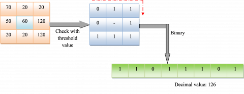
LGP [16]: It employs the gradient values of the eight neighboring pixels of a specified pixel computed as the absolute values of intensity variations among the specific pixel and their neighboring pixels. When the gradient value of their neighbor is higher than the threshold value, then a pixel is considered a value as 1; else, it is considered as 0. The code of LGP is attained using the integration of the binary values of 1s and 0s into a binary code for the specified pixel, which is given in Figure 3.
Figure 3. LGP feature extraction for the proposed model
A circular neighborhood of radius ra is assumed that is centered on a particular pixel. On the circle, neighboring pixels are taken as pl. The gradient value among a central pixel xcp and their neighbor xne is fixed as given in Eq. (3).
$g{}_{ne}=\left| x{}_{ne}-x{}_{cp} \right|$ (3)
The average of pl gradient values is computed in Eq. (4).
$\bar{g}=\frac{1}{pl}\sum\limits_{ne=0}^{pl-1}{g{}_{ne}}$ (4)
Therefore, the LGP descriptor is computed in Eq. (5).
$LG{{P}_{pl,ra}}=\sum\limits_{ne=0}^{pl-1}{sg\left( g{}_{ne}-\bar{g} \right)}{{2}^{ne}}$ (5)
$sg\left( x \right)=\left\{ \begin{matrix} 0 & x<0 \\ 1 & x\ge 0 \\\end{matrix} \right.$ (6)
The LGP features are obtained using this descriptor. Therefore, the combination of attained features at the extraction stage is given as $F e_{f b}=\left\{f e^{H O G}, f e^{L G P}\right\}$, where $f b=1,2, \cdots, N o$.
3.4 Dimensionality reduction using PCA
The extracted features $F e_{f b}$ are given to this PCA [17] for obtaining the features as principle component. Here, the extracted higher dimensional features are converted into the lower dimensional features. The PCA is computed by following steps. Consider the data matrix as $F e_{f b} \leftarrow S u$ with Va variables or the number of feature values for each pixel and No of observations. The PCA-based dimension reduction is computed in Eq. (7).
$P c=Q^{\prime} S u$ (7)
Here, the values of Pc is the principal components designed as weighted average of original sample vectors. The term Q is determined from the covariance matrix CM as given in Eq. (8).
$Q=E v \cdot D m^{-\frac{1}{2}}$ (8)
In Eq. (8), the terms Ev and Dm denotes the matrix of eigenvectors of CM and diagonal matrix of the eigenvalues of CM. Assume AB as the matrix of No´Va with noth column as $S u_{n o}-\beta$.
$A B=\left[S u_{1}-\beta, . ., S u_{N o}-\beta\right]$ (9)
Here, the mean vector is termed as β that is computed $\beta=\frac{1}{N o}\left(S_{1}+\ldots+S_{N o}\right)$ and CM is computed with size of Va´Va, which is given in Eq. (10).
$C M=\frac{1}{N o-1} A B \cdot A B^{T}$ (10)
Finally, the obtained principal components are denoted as $p c a(S u, N P)$ and the term NP is the number of preserved principal components. The attained PCA reduced features is denoted as $F e_{f b}^{P C A}$.
4.1 Training data formation
The input video frames are converted into three types of patterns in the proposed automated anomaly detection and localization. Consider Zij videos, in which ijjth video is involved with GF counts of frames. Let gffi indicates the total number of frames in a video, where, fi=1,2,…GF. Eq. (11) shows the pattern 1 formation on the basis of consecutive frames, Eq. (12) shows the pattern 2 formation on the basis of skipping one frame after one (GF(T) shows the total frames in pattern 2), and Eq. (13) shows the pattern 3 formation on the basis of skipping five frames after one (GF(v) shows the total frames in pattern 3). These three patterns are categorized for processing for feature extraction using HOG, and LGP in order to develop the proposed anomaly detection and localization in videos.
pattern $1=\left\{g f_{1}, g f_{2}, \cdots, g f_{G F}\right\}$ (11)
pattern $2=\left\{g f_{1}, g f_{3}, g f_{5}, \cdots, g f_{G F^{(T)}} \,\,\right\}$ (12)
pattern $3=\left\{g f_{1}, g f_{5}, g f_{15}, \cdots, g f_{G F^{(F)}} \,\, \right\}$ (13)
4.2 Self-organizing map
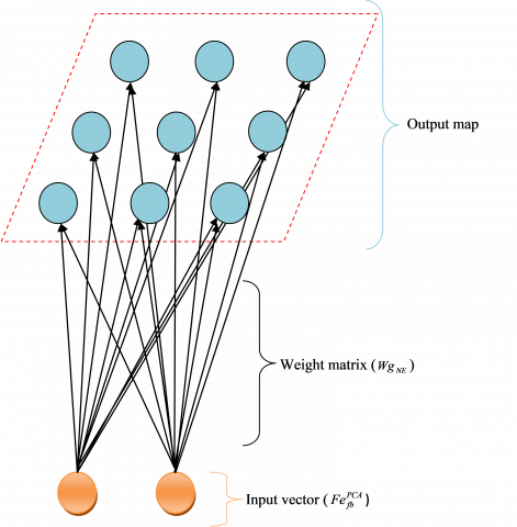
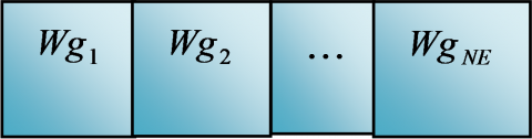
The SOM [16] is used to categorize video features into normal and abnormal classes. The combined extracted features are converted into understandable information for determining whether a test observation is an anomaly or not using SOM. It is also called Kohonen NN, which is one type of unsupervised machine learning approach. It is done by creating a network, which keeps information on the topological relationships within the training data. A SOM structure includes several neurons, where each neuron is indicated with a weight vector, which consists of a similar dimension of the training data. The organization of neurons is performed based on their similarity, in which the equivalent weight vectors are formed as groups named neighbors. This neighborhood relationship denotes the map structure that reveals the correlation in the training data. A SOM is created using the normalization of input data by calculating the z-score at every observation. Furthermore, the determination of the size of the map is done by computing the number of neurons from the entire observations in training data, which is given in Eq. (14).
$N E \approx 5 \sqrt{N o}$ (14)
Here, the terms No and NE denotes the number of observations and the number of neurons, respectively. The neurons are formed in a 2-dimensional map, where the ratio of the side lengths of the map is about the ratio of the two largest eigenvalues of the covariance matrix of training data. Initially, the elements of the weight vectors are randomly created for each neuron. Further, Euclidean distance is computed among entire neurons, where the minimal distance of neuron is found that is named Best Matching Unit (BMU). Therefore, the selection of neighbors of the BMU is determined, and its weight vectors are updated through a neighborhood function as given in Eq. (15).
$N f_{b m n r}(i)=\eta(i) e^{\left(-\frac{\left\|v e_{b m}-v e_{n r}\right\|}{2 \Re^{2}(i)} \quad \right)}$ (15)
In Eq. (15), the neighborhood function is termed as Nfbmnr among the BMU bm and a neuron nr, the vector of neuron is mentioned as venr, the radius around bm is termed as $\Re$ and the vector of the BMU is mentioned as vebm. The index of iterations of training is represented as i and the learning rate is represented as η. The neurons are updated using Eq. (16).
$W{{g}_{nr}}\left( i+1 \right)=W{{g}_{nr}}\left( i \right)+N{{f}_{bmnr}}\left( i \right)\left[ Fe_{fb}^{PCA}\left( i \right)-W{{g}_{nr}}\left( i \right) \right]$ (16)
Here, the weight vectors of neuron nr are termed as $W g_{n r}(i)$ at ith iteration of training and the input observation of the BMU bm is denoted as $F e_{f b}^{P C A}(i)$. The training of SOM is done iteratively when the grouping of all the weight vectors of the map are transformed into clusters based on their distance. The SOM is formed until the learning process is over. The structure of SOM is represented in Figure 4.
Figure 4. SOM structure for proposed model
4.3 Optimized self organizing map
The weight of the SOM network is optimized for the proposed model using FOA, which is given in Figure 5.
Figure 5. Optimized SOM structure
The term $W g_{n r}$ denotes the weight of the input vector of SOM, where $n r=1,2, \ldots, N E$ and NE indicates the total weight which is equal to the total neurons. Here, the weight is optimized in certain percentages within the bounding limit of -20% to +20%. The proposed automated anomaly detection and localization in videos use the new updated weight function to update new weights using Eq. (17).
$W g_{n r}=W g_{n r}+\left(W g_{n r}+\frac{s o l}{100}\right)$ (17)
Here, the term sol shows the solution. The proposed model's major objective is to maximize the precision of the objective function, and it is represented in Eq. (18).
$O B F=\underset{\left\{W g_{n r}\right\}}{\arg \max }( precision )$ (18)
Here, the precision of the proposed model is termed as precisior and the objective function of the proposed anomaly detection model is specified as OBF. Precision is defined as “the ratio of positive observations that are predicted exactly to the total number of observations that are positively predicted” that is given in Eq. (19).
precision $=\frac{p o^{ {true }}}{p o^{ {true }}\quad+n e^{ {false }}}$ (19)
Here, $po^{true}$ and $n e^{ {false }}$ refer to the true positives and false positives, respectively.
4.4 FOA
FOA [18] is implemented for better training of SOM in the proposed automated anomaly detection and localization in videos. It is proposed based on the hunting behavior of fruit flies towards their food source. This fruit fly has better perception and sensing behavior. It is a famous and eminent algorithm due to its simple structure, and it is efficient due to the generation of new candidate solutions. The structure of FOA is separated into seven steps using the characteristics of food hunting. It is formulated below. Initially, the parameters are initialized that are “total evolution number, the population size pop, and the initial fruit fly swarm location,” where the location is mentioned as $\left(Y_{0}, Z_{0}\right)$. Secondly, the population is formulated below.
$Y_{t}=Y_{0}+$ rand (20)
$Z_{t}=Z_{0}+$ rand (21)
The computation of smell Sm and distance Di is formulated in Eq. (22) and Eq. (23).
$S m_{t}=\frac{1}{D i_{t}}$ (22)
$D i_{t}=\sqrt{Y_{t}^{2}+Z_{t}^{2}}$ (23)
Moreover, the fitness function is determined with the concentration of smell as given in Eq. (24).
Smell $_{t}=f f\left(S m_{t}\right)$ (24)
Here, ff denotes the fitness function and determine the maximum individual fruit fly in the fruit fly swarm is given in Eq. (25).
$[bestSmell\_bestindex] =\max ( Smell)$ (25)
The selection operation is performed using Eq. (26).
$f f_{\text {best }}= best \_Y$ (26)
$Y_{b e s t}=Y( bestindex )$ (27)
$Z_{\text {best }}=Z(bestindex)$ (28)
Therefore, the implementation is executed until it satisfies the condition. The pseudo code of the FOA is represented in Algorithm 1.
|
Algorithm 1: FOA [18] |
|
Initialize population |
|
Initialize parameters |
|
Crossover with best known swarm food location |
|
Evaluate the fruit flies |
|
If $bestSmell<Smellbest$ |
|
Whether the termination condition is satisfied |
|
else |
|
update location of best swarm |
|
end if |
|
end |
4.5 Anomaly localization
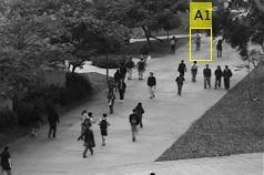
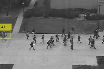
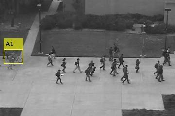
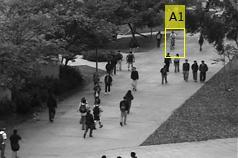
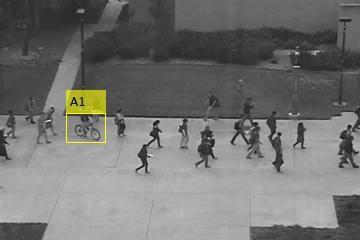
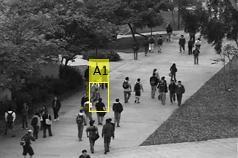
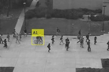
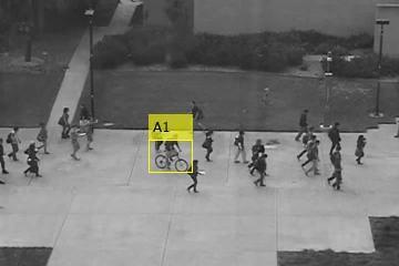
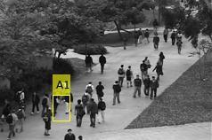
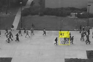
Once the anomaly is detected in a video by the proposed FOA-SOM, the localization of the anomaly in that video is performed by the flow of objects and their directions. For the frames containing an anomaly, the distance of pixels is computed between each frame. If the distance exceeds a certain threshold Hd, the concerning point is localized as an anomaly, and the object with the highest distance is marked with a yellow bounding box. Similarly, the movement of objects in the video is observed. If the direction is rather than the movements of other objects, the localization has to be done to a certain point.
5.1 Experimental setup
The proposed automated anomaly detection and localization in videos were carried out in MATLAB 2019a. The population was considered as ten, and the maximum number of iterations was considered as 100. The performance was analyzed with conventional models like SOM [16], Fire Fly (FF)-SOM [19], Particle Swarm Optimization (PSO-SOM) [20], and FOA-SOM. The proposed model was compared with the state-of-the-art techniques on two datasets from UCSD.
5.2 Performance metrics
Some of the performance measures considered for the proposed model is listed below. Here, $po^ {true}, ne^{true}, po^{false}, ne^{false}$ refer to the true positives, true negatives, false positives, and false negatives respectively.
(a) Accuracy: Ratio of the observation of exactly predicted to the whole observations.
$A c=\frac{\left(p o^{ {true }}\quad+n e^{ {trie }}\quad\right)}{\left(p o^{ {true }}\quad+n e^{ {true }}\quad+p o^{ {false }}\quad+n e^{ {false }}\quad\right)}$ (29)
(b) F1 score: Harmonic mean between precision and recall. It is used as a statistical measure to rate performance.
$F 1 score=\frac{ { Recall } \cdot { precision }}{ { precision }+\operatorname{Re} { call }}$ (30)
(c) MCC: Correlation coefficient computed by four values.
$M C C=\frac{p o^{ {true }} \quad\times n e^{ {true }}\quad-p o^{{false }} \quad\times n e^{ {false }}}{\sqrt{\left(p o^{ {true }}\quad+p o^{ {false }}\quad\right)\left(p o^{ {true }}\quad+n e^{ {false }}\quad\right) \left(n e^{ {true }}\quad+p o^{ {false }}\quad\right)\left(p o^{ {true }}\quad+n e^{ {false }}\quad\right)}}$ (31)
(d) Recall: The number of true positives divided by the total number of elements that actually belong to the positive class.
$\operatorname{Re} c a l l=\frac{p o^{ {trule }}}{p o^{ {true }}\quad+n e^{ {false }}}$ (32)
5.3 Experimental output
The final output for the proposed model in videos is given in Figure 6. The figure presents output frame-wise in two videos from both datasets. It represents frames initially with no anomaly and then the frames with an anomaly. The highlighted yellow bounding box represents Anomaly detected in that frame.
|
Frames |
Video 1 |
Frames |
Video 2 |
|
Frame-2 |
Frame-2 |
||
|
Frame-92 |
Frame-61 |
||
|
Frame-94 |
Frame-73 |
||
|
Frame-98 |
Frame-98 |
||
|
Frame-176 |
Frame-118 |
||
|
Frame-183 |
Frame-132 |
||
|
Frame-190 |
Frame-165 |
||
|
Frame-194 |
Frame-179 |
Figure 6. Experimentation results of the proposed model for 2 videos
5.4 Convergence analysis
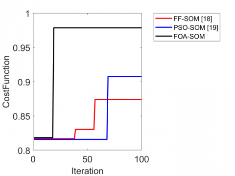
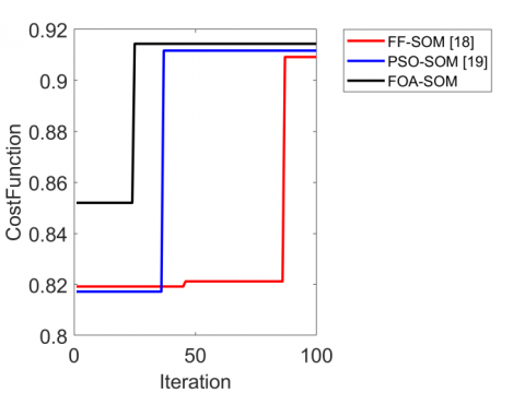
The convergence of the proposed anomaly detection and localization in videos is analyzed in terms of the cost function (precision) and iterations that are represented in Figure 7. The FOA-based optimized SOM attains better performance at the 20th iteration. The FOA-SOM is 18% and 17% enhanced than FF-SOM and PSO-SOM, respectively, for dataset 1 at the 50th iteration. Likewise, the performance of the FOA-SOM on dataset 2 is 0.1% and 10.9% superior to FF-SOM and PSO-SOM, respectively, at the 50th iteration. Thus, the performance of the proposed automated anomaly detection and localization model using FOA-based optimized SOM is superior to other algorithms.
(a)
(b)
Figure 7. Precision analysis of the proposed model for (a) Dataset 1 and (b) Dataset 2
5.5 Confusion matrix
The confusion matrix of the proposed model is given in Figure 8. Which attains true positive value as the 447, false-positive value as 18, false-negative value as 9, and true negative values as 582.
Figure 8. Confusion matrix for the proposed model
5.6 Overall performance analysis
The overall performance of the proposed model using FOA-SOM is enhanced than other conventional models for dataset 1 and dataset 2 that are represented in Table 1 and Table 2, respectively. For dataset 1, the accuracy of the FOA-SOM is 3.7%, 1.5%, and 0.78% improved than SOM, FF-SOM, and PSO-SOM, respectively. The recall of the FOA-SOM is 0.6% enhanced than SOM, 0.22% enhanced than FF-SOM, and 0.67% enhanced than PSO-SOM for dataset 1. The F1-score of the FOA-SOM is 3.7%, 1.8%, and 0.59% advanced than SOM, FF-SOM, and PSO-SOM, respectively, for dataset 2. Therefore, the proposed model using FOA-SOM establishes better performance than conventional models.
Table 1. Overall performance analysis of the proposed model in videos for Dataset 1
|
Measures |
SOM |
FF-SOM |
PSO-SOM |
FOA-SOM |
|
Accuracy |
0.93939 |
0.95928 |
0.96686 |
0.97443 |
|
Recall |
0.97368 |
0.97807 |
0.97368 |
0.98026 |
|
Precision |
0.89516 |
0.93111 |
0.95075 |
0.96129 |
|
F1-score |
0.93277 |
0.95401 |
0.96208 |
0.97068 |
|
MCC |
0.88035 |
0.91841 |
0.93286 |
0.94816 |
Table 2. Overall performance analysis of the proposed model in videos for Dataset 2
|
Measures |
SOM |
FF-SOM |
PSO-SOM |
FOA- SOM |
|
Accuracy |
0.91132 |
0.92735 |
0.93803 |
0.94338 |
|
Recall |
0.90693 |
0.93939 |
0.96104 |
0.97186 |
|
Precision |
0.91285 |
0.91561 |
0.91736 |
0.9182 |
|
F1-score |
0.90988 |
0.92735 |
0.93869 |
0.94427 |
|
MCC |
0.82262 |
0.85501 |
0.87709 |
0.8883 |
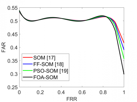
5.7 ROC analysis
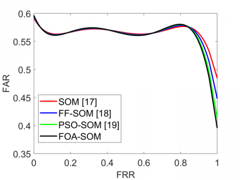
The Receiver Operating Characteristics (ROC) curve demonstrates "the tradeoff between the true positive and false-positive fractions," shown in Figure 9. The ROC curve relies on the diagonal line to show the proposed model's performance. The proposed FOA-SOM achieves better performance than conventional models.
(a)
(b)
Figure 9. ROC analysis of the anomaly detection and localization for (a) Dataset 1 and (b) Dataset 2
This paper has developed a new automated anomaly detection and localization model using optimized SOM in crowd videos. It was done by generating three different patterns of video frames followed by adopting a feature extraction process. The features were extracted from the inputs using approaches like HOG and LGP and PCA dimensionality reduction. Moreover, the meta-heuristic training-based SOM was employed for the detection and localization process. The training of SOM is improved by using FOA. Finally, the flow of objects and directions is analyzed for anomaly localization. From the experimental analysis, the proposed FOA-SOM was 3.5%, 1.7%, and 0.57% enhanced than SOM, FF-SOM, and PSO-SOM, respectively. Thus, the outcome of the proposed model using FOA-SOM has established better performance than the existing models.
|
Abbreviations |
Descriptions |
|
CCTV |
Closed-Circuit Television |
|
CNN |
Convolutional Neural Network |
|
PCANet, |
Principal Component Analysis Network |
|
SL-HOF |
Spatially Localized Histogram of Optical Flow |
|
GAN |
Generative Adversarial Networks |
|
SOM |
Self-Organizing Map |
|
OF |
Optical Flow |
|
LGP |
Local Gradient Pattern |
|
RBMs |
Restricted Boltzmann Machines |
|
ULGP-OF |
Uniform Local Gradient Pattern Based Optical Flow |
|
MCLs |
Motion Convolutional Layers |
|
BMU |
Best Matching Unit |
|
HOG |
Histogram Of Oriented Gradients |
|
GMM |
Gaussian Mixture Model |
|
RL |
Reinforcement Learning |
|
OCELM |
One-Class Extreme Learning Machine |
|
GPR |
Gaussian Process Regression |
|
STIPs |
Sparse Spatio-Temporal Interest Points |
|
EW |
Edge Wrapping |
|
GMFC-VAE |
Gaussian Mixture Fully Convolutional-Variational Autoencoder |
|
AICN |
Adaptive Intra-Frame Classification Network |
|
ARPL |
Adaptive Region Pooling Layer |
|
DSTN |
Deep Spatiotemporal Translation Network |
|
SCLs |
Shape Convolutional Layers |
[1] Li, W., Mahadevan, V., Vasconcelos, N. (2013). Anomaly detection and localization in crowded scenes. IEEE Transactions on Pattern Analysis and Machine Intelligence, 36(1): 18-32. https://doi.org/10.1109/TPAMI.2013.111
[2] Sabokrou, M., Fathy, M., Hoseini, M. (2016). Video anomaly detection and localisation based on the sparsity and reconstruction error of auto-encoder. Electronics Letters, 52(13): 1122-1124. https://doi.org/10.1049/el.2016.0440
[3] Chouhan, N., Khan, A. (2019). Network anomaly detection using channel boosted and residual learning based deep convolutional neural network. Applied Soft Computing, 83: 105612. https://doi.org/10.1016/j.asoc.2019.105612
[4] Nawaratne, R., Alahakoon, D., De Silva, D., Yu, X. (2019). Spatiotemporal anomaly detection using deep learning for real-time video surveillance. IEEE Transactions on Industrial Informatics, 16(1): 393-402. https://doi.org/10.1109/TII.2019.2938527
[5] Xiao, Z., Fang, H., Wang, X. (2020). Nonlinear polynomial graph filter for anomalous IoT sensor detection and localization. IEEE Internet of Things Journal, 7(6): 4839-4848. https://doi.org/10.1109/JIOT.2020.2971237
[6] Iakovidis, D.K., Georgakopoulos, S.V., Vasilakakis, M., Koulaouzidis, A., Plagianakos, V.P. (2018). Detecting and locating gastrointestinal anomalies using deep learning and iterative cluster unification. IEEE Transactions on Medical Imaging, 37(10): 2196-2210. https://doi.org/10.1109/TMI.2018.2837002
[7] Sabokrou, M., Fayyaz, M., Fathy, M., Klette, R. (2017). Deep-cascade: Cascading 3d deep neural networks for fast anomaly detection and localization in crowded scenes. IEEE Transactions on Image Processing, 26(4): 1992-2004. https://doi.org/10.1109/TIP.2017.2670780
[8] Shi, X., Qiu, R., He, X., Ling, Z., Yang, H., Chu, L. (2020). Early anomaly detection and localisation in distribution network: A data-driven approach. IET Generation, Transmission & Distribution, 14(18): 3814-3825.
[9] Ratre, A., Pankajakshan, V. (2018). Tucker tensor decomposition‐based tracking and Gaussian mixture model for anomaly localisation and detection in surveillance videos. IET Computer Vision, 12(6): 933-940. https://doi.org/10.1109/TIP.2017.2670780
[10] Wang, S., Zhu, E., Yin, J., Porikli, F. (2018). Video anomaly detection and localization by local motion based joint video representation and OCELM. Neurocomputing, 277: 161-175. https://doi.org/10.1016/j.neucom.2016.08.156
[11] Ganokratanaa, T., Aramvith, S., Sebe, N. (2020). Unsupervised anomaly detection and localization based on deep spatiotemporal translation network. IEEE Access, 8: 50312-50329. https://doi.org/10.1109/ACCESS.2020.2979869
[12] Fan, Y., Wen, G., Li, D., Qiu, S., Levine, M.D., Xiao, F. (2020). Video anomaly detection and localization via gaussian mixture fully convolutional variational autoencoder. Computer Vision and Image Understanding, 195: 102920. https://doi.org/10.1016/j.cviu.2020.102920
[13] Cheng, K.W., Chen, Y.T., Fang, W.H. (2015). Gaussian process regression-based video anomaly detection and localization with hierarchical feature representation. IEEE Transactions on Image Processing, 24(12): 5288-5301. https://doi.org/10.1109/TIP.2015.2479561
[14] Xu, K., Sun, T., Jiang, X. (2019). Video anomaly detection and localization based on an adaptive intra-frame classification network. IEEE Transactions on Multimedia, 22(2): 394-406. https://doi.org/10.1109/TMM.2019.2929931
[15] Kobayashi, T., Hidaka, A., Kurita, T. (2007). Selection of histograms of oriented gradients features for pedestrian detection. In International Conference on Neural Information Processing, 4985: 598-607. https://doi.org/10.1007/978-3-540-69162-4_62
[16] Saad, S., Sagheer, A. (2015). Difference-based local gradient patterns for image representation. In International Conference on Image Analysis and Processing, 9280: 472-482. https://doi.org/10.1007/978-3-319-23234-8_44
[17] Kang, X., Xiang, X., Li, S., Benediktsson, J.A. (2017). PCA-based edge-preserving features for hyperspectral image classification. IEEE Transactions on Geoscience and Remote Sensing, 55(12): 7140-7151. https://doi.org/10.1109/TGRS.2017.2743102
[18] Pan, W.T. (2012). A new fruit fly optimization algorithm: Taking the financial distress model as an example. Knowledge-Based Systems, 26: 69-74. https://doi.org/10.1016/j.knosys.2011.07.001
[19] Yang, X.S. (2013). Multiobjective firefly algorithm for continuous optimization. Engineering with Computers, 29(2): 175-184. https://doi.org/10.1007/s00366-012-0254-1
[20] Bonyadi, M.R., Michalewicz, Z. (2015). Analysis of stability, local convergence, and transformation sensitivity of a variant of the particle swarm optimization algorithm. IEEE Transactions on Evolutionary Computation, 20(3): 370-385. https://doi.org/10.1109/TEVC.2015.2460753