Youkun Cheng | Zhenwu Shi* | Fajin Zu
© 2020 IIETA. This article is published by IIETA and is licensed under the CC BY 4.0 license (http://creativecommons.org/licenses/by/4.0/).
OPEN ACCESS
In special areas, the highways may suffer from such diseases as deformation, cracking, subsidence, and potholes, making highway maintenance a complex and difficult task. To obtain the law-term deformation law of the subgrade and accurately evaluate the subgrade and pavement stability, this paper establishes a subgrade stability evaluation model based on artificial neural network (ANN). Firstly, the law of unstable subgrade deformation in highways of special areas was derived by analyzing the influencing factors on subgrade stability, namely, temperature field, moisture field, and traffic load. Next, the correlations between input and output characteristic quantities were extracted, and used to construct the nonredundant mapping function between influencing factors of subgrade unstable deformation and the levels of subgrade stability. Finally, a fuzzy neural network (FNN) was constructed based on Takagi-Sugeno model, realizing the evaluation of subgrade stability. The proposed model was proved effective and accurate through experiments.
fuzzy neural network (FNN), subgrade stability evaluation, Takagi-Sugeno model, special areas
The infrastructure boom in China has created a nationwide network of interconnected highways. However, the highways in special areas (e.g., mountains, hills, watersides, and permafrost regions) may suffer from subgrade and pavement diseases, such as deformation, cracking, subsidence, and potholes, under the combined effects of the particular soil properties and the traffic load [1-3]. In these special areas, it is a complex and difficult task to maintain the highways. Besides, traffic accidents are very likely to occur on the highways with subgrade and pavement diseases. Therefore, it is of high necessity to analyze and evaluate the stability of highway subgrade and pavement in special areas.
Since the 1980s, foreign scientists have explored typical subgrade diseases in various special areas [4-5]. For instance, Rabab’ah et al. [6] investigated cases of subgrade and pavement diseases in frozen soil areas of Alaska, and attributed the longitudinal cracks of subgrade and those of pavement to frost heave and thaw settlement, respectively. Chinese researchers have studied subgrade and pavement diseases on the Qinghai-Tibet Highway, namely, uneven deformation, subsidence, and horizontal/vertical cracks [7-9]. Tavakol et al. [10] summarized and analyzed the disease features of highway subgrade and pavement, and ascribed the diseases to objective factors like harsh weather and melting of frozen soil. Chibuzor and Van Duc [11] constructed the finite-element temperature field of the highway, and identified the rise of frozen soil temperature as the key cause of longitudinal cracking in subgrade and pavement.
Many scholars have successfully investigated the relationship between highway subgrade and pavement diseases and traffic load through theoretical analysis, modeling simulation, and experimental verification [12-15]. Based on double-layer foundation model, Neupane et al. [16] examined the deformation features of expressway subgrade under asymmetric traffic load following the idea of mobile constant load, and discussed the influence of traffic load amplitude and load movement speed on subgrade deformation in the case of saturated soil. Mishra et al. [17] used linear elastic and elastoplastic models to simulate the reinforced soft soil subgrade, and obtained the deformation attenuation of the subgrade under different driving frequencies and vehicle load amplitudes through comparative analysis.
Abundant experimental evidences show that the subgrade fill is generally unsaturated even after compaction. Therefore, many efforts have been paid to analyze the slope stability under the rainfall infiltration of subgrade [18-21]. Based on the permeability comparison of unsaturated and saturated soils by Daud et al. [22], Yadav et al. [23] empirically determined the water permeability range of the subgrade slope fill, and obtained the soil-water characteristic curve by analyzing the time trend of water content of the slope fill. Drawing on the theory of unsaturated soil strength, Aneke et al. [24] conducted finite-element analysis of the stability of subgrade slopes with unsaturated soil, and experimentally proved that, under continued rainfall, the stability of subgrade slopes plunged initially and quickly tended to be stable.
In terms of solving differential settlement by widening subgrade, Ikeagwuani et al. [25] analyzed the mechanism and effect of subgrade widening technique in reconstruction and expansion projects, highlighting the importance of mitigating and controlling differential settlement of subgrade according to pile-soil interaction, and pavement deformation mechanism.
To sum up, the existing studies differ in direction, adaptability, and completeness, as they deal with different types of subgrade diseases and the subgrade stability is affected by varied factors. The previous research rarely tackles the long-term deformation of subgrade. The mechanical parameters calculated by small sample tests on subgrade and pavement deformation are of little practical value. To overcome these defects, this paper constructs a subgrade stability evaluation model based on artificial neural network (ANN), which can approximate the nonlinear function mapping in actual problems at any accuracy.
The remainder of this paper is organized as follows: Section 2 analyzes the trends of temperature field, moisture field, and traffic load of the subgrade, and draws the law of unstable subgrade deformation in special areas; Section 3 extracts the correlations between input and output characteristic quantities, and selects the optimal characteristic quantities of subgrade stability, facilitating the construction of the nonredundant mapping function between influencing factors of subgrade unstable deformation and the levels of subgrade stability; Section 4 establishes a fuzzy neural network (FNN) based on Takagi-Sugeno model, realizing the evaluation of subgrade stability; Section 5 proves the effectiveness and accuracy of the proposed model; Section 6 puts forward the conclusions.
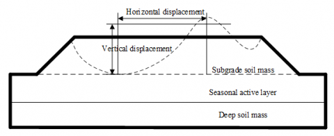
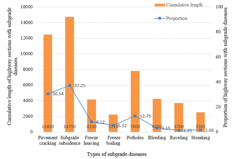
In special areas, the highway subgrade is greatly affected by three factors: ambient temperature, soil moisture, and traffic load. Figure 1 illustrates the unstable deformation of subgrade cross section. Figure 2 sums up the diseases of the target highway section. The physical-mechanical properties of the subgrade change with the seasonal variation in atmospheric temperature and rainfall, leading to various diseases like deformation, horizontal/vertical cracking, potholes, and local subsidence. To master the law of unstable subgrade deformation in highways in special areas, it is of great necessity to explore the trends of the temperature field, moisture field, and traffic load of the subgrade.
Figure 1. The unstable deformation of subgrade cross section
Figure 2. The diseases of the target highway section
2.1 Temperature influence
The highway subgrade was likened to a plane. Following the principle of thermodynamics, the partial differential equation of heat conduction for the unsteady temperature field can be established as:
$\frac{\partial {{T}_{RT}}}{\partial t}=\frac{\alpha }{\rho {{C}_{p}}}\left( \frac{{{\partial }^{2}}{{T}_{RT}}}{\partial {{a}^{2}}}+\frac{{{\partial }^{2}}{{T}_{RT}}}{\partial {{b}^{2}}}+\frac{HS{{I}_{in}}}{\alpha } \right)$ (1)
where, TRT is the real-time temperature of the subgrade; t is the time of head conduction; α, ρ, and Cp are the thermal conductivity, density, and specific heat at constant pressure of the subgrade, respectively; HSIin is the intensity of the heat source in the subgrade; a and b are the position of each coordinate point.
With the seasonal changes, the subgrade soil undergoes a cyclic process from freezing in winter to heating in summer. Considering phase change, formula (1) can be optimized as:
$\begin{align} & \rho {{C}_{p}}\frac{\partial {{T}_{RT}}}{\partial t}=\frac{\partial }{\partial a}\left( \alpha \frac{\partial {{T}_{RT}}}{\partial a} \right)+ \\ & \frac{\partial }{\partial b}\left( \lambda \frac{\partial {{T}_{RT}}}{\partial b} \right)+HS{{I}_{in}}+\rho \cdot LH\cdot \frac{\partial {{r}_{sp}}}{\partial t} \\\end{align}$ (2)
where, LH is the latent heat of phase change of subgrade soil from freezing to heating. In the absence of phase change, the temporal variation rate of the solid phase ratio rsp is zero. In view of the climate features of special areas and the local temperature, the boundary conditions for the heat flow distribution and heat convection of the highway subgrade temperature field based on the principle of heat transfer theory were defined as the superposition between solar radiation, subgrade/pavement counter radiation, and heat convection in the air. Then, the analytical solution of the subgrade temperature field without considering the phase change can be expressed as:
$T_{R T}(a, t)=T_{a v}+R_{R B} e^{-a \sqrt{\frac{\omega}{2 \alpha}} \cos \left(\omega t-a \sqrt{\frac{\omega}{2 \alpha}}\right)}$ (3)
where, Tav is the mean temperature of the subgrade; θ is the angular frequency; RRB and RP are the temperature change amplitudes of the subgrade and pavement, respectively.
2.2 Moisture influence
The soil-water potential P, which characterizes water migration in the subgrade soil, is generally composed of gravitational potential Pg, pressure potential Pp, matrix potential Pm, solute potential Ps, and temperature potential PT. The core components are Pg, Pm, and PT. The moisture flow from high to low positions in the unsaturated subgrade soil can be described by Darcy’s law:
$\begin{matrix} TF=-H\left( P \right)\nabla P & or & TF=-H\left( \tau \right)\nabla P \\\end{matrix}$ (4)
where, TF is the water transport flux in the soil; H and τ are the hydraulic conductivity and moisture content of the unsaturated soil, respectively. Let WD be the moisture diffusivity of unsaturated soil. Then, the governing equation of soil moisture migration in the highway subgrade can be expressed as:
$\begin{align} & \frac{\partial \tau }{\partial t}=\frac{\partial }{\partial a}\left[ WD\left( \tau \right)\frac{\partial \tau }{\partial a} \right]+\frac{\partial }{\partial b}\left[ WD\left( \tau \right)\frac{\partial \tau }{\partial b} \right] \\ & +\frac{\partial }{\partial a}\left[ \eta \frac{\partial \tau }{\partial a} \right]+\frac{\partial }{\partial b}\left[ \eta \frac{\partial \tau }{\partial b} \right]+\frac{\partial }{\partial b}\left[ H\left( \tau \right) \right]-\frac{\partial {{r}_{sp}}}{\partial t} \\\end{align}$ (5)
where, η is the parameter reflecting the correlation between soil properties and moisture migration rate. The moisture migration in subgrade soil has much to do with soil temperature. The solid phase ratio rsp can be calculated by formula (2), while the moisture content τ can be calculated by:
$\tau =p{{T}_{RT}}^{-q}$ (6)
where, p and q are empirical parameters about soil properties. Formulas (2), (5), and (6) constitute the coupling model between temperature field and moisture field of highway subgrade.
There are two kinds of boundary conditions of subgrade moisture field: the distribution of moisture content τ on subgrade surface, and the water flux Fws on subgrade surface. Rainfall and evaporation belong to the latter type of boundary conditions. The solution after the n+1-th iteration can be obtained by:
$x_{n+1}(\tau, t)=-\int_{\tau}^{\tau_{B}} \frac{W D(y)}{H(y)-\int_{\tau_{0}}^{y} \frac{\partial x_{n}\left(\tau^{\prime}, t\right)}{\partial t} d \tau^{\prime}} d y$ (7)
where, τ0 and τB are the initial moisture content and boundary moisture content on subgrade surface, respectively. Meanwhile, we have:
${{x}_{2}}(\tau ,t)=-\int{_{\tau }^{{{\tau }_{B}}}}\frac{WD(y)}{H(y)-{{F}_{ws}}\frac{y\text{-}{{\tau }_{0}}}{{{\tau }_{B}}(t)-{{\tau }_{0}}}}dy$ (8)
After solving x2(τ, t) by formula (8), x3(τ, t), x4(τ, t)… can be calculated by formula (7).
2.3 Traffic load influence
Under the combined action of its own weight and traffic load, highway subgrade undergoes unstable elastoplastic deformation. Table 1 lists the daily traffic volume in the target highway section. Drawing on the elastoplastic principle, the Mohr-Coulomb model was taken as the constitutive model to calculate the cumulative plastic deformation of the highway subgrade. Let λ, s, f, and β be the shear strength, cohesion, normal stress, and internal friction angle of the subgrade, respectively. Then, the strength criterion of the Mohr-Coulomb model can be expressed as:
Table 1. The daily traffic volume in the target highway section
|
Year |
2010 |
2011 |
2012 |
2013 |
2014 |
2015 |
2016 |
2017 |
2018 |
2019 |
Mean |
|
Daily traffic volume |
523 |
557 |
670 |
742 |
598 |
688 |
719 |
732 |
759 |
780 |
677 |
$\lambda =s\text{-}f\tan \beta $ (9)
The increment of the elastoplastic strain tensor can be expressed as:
$\Delta ST=\Delta S{{T}_{et}}+\Delta S{{T}_{pt}}$ (10)
where, ΔSTet and ΔSTpt are the tensor increments of elastic strain and plastic strain, respectively. Let εds be the Mohr-Coulomb deviatoric stress coefficient. Then, the force surface equation of the Mohr-Coulomb model during stress bending can be expressed by the following strain invariant:
${{F}_{s}}={{\varepsilon }_{ds}}{{S}_{VM}}-{{S}_{p}}\tan \beta -s=0$ (11)
where, SVM is the equivalent stress subject to the Von Mises yield criterion; Sp is the equivalent compressive stress.
Figure 3. The pulse form illustration of traffic load contacting subgrade and pavement
Note: Δt is the interval between two vehicles contacting the same subgrade; Loadmax is the real-time maximum traffic load acting on the subgrade.
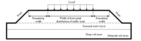
Considering the difficulty in simulating the constantly changing action of traffic load on subgrade, the traffic load contacting subgrade and pavement was simulated in the pulse form (Figure 3). The distribution of traffic load acting on the subgrade is presented in Figure 4. Each vehicle on the highway exerts a load on the subgrade in a very short time. The duration of load application can be calculated by:
${{T}_{DL}}=\frac{12{{r}_{T}}}{v} $ (12)
where, rT is the tire radius of the vehicle; v is the driving speed. The traffic load from the vehicle passing the highway subgrade can be calculated by:
$Load\left( t \right)=Loa{{d}_{\max }}\cdot \sin {{\left( \frac{\pi t}{{{T}_{s}}} \right)}^{2}}$ (13)
where, Ts is the duration of load application of a single vehicle on the subgrade.
Figure 4. The distribution of traffic load acting on the subgrade
The collected data on ambient temperature, soil moisture, and traffic load from the target subgrade contain important information that determine the stability of highway subgrade. To accurately evaluate the instantaneous and long-term stability of the subgrade, it is necessary to introduce artificial intelligence (AI) technology to realize autonomous and adaptive learning of this information.
With the help of the self-learning and adaptive advantages of artificial intelligence (AI), this information can realize accurate analysis and evaluation of the instantaneous and long-term stability of roadbed projects. Thus, this paper attempts to build up the nonredundant mapping function between influencing factors of subgrade unstable deformation and the levels of subgrade stability, with the aid of the ANN. The premise is to effectively extract the correlations between input and output characteristic quantities. Let NS be the number of input samples. Then, the input and output characteristic quantities A and B can be expressed as:
$\left\{ \begin{align} & A={{\left( {{A}_{1}},{{A}_{2}},...,{{A}_{{{N}_{S}}}} \right)}_{X\times {{N}_{S}}}} ,{{A}_{i}}={{\left( {{A}_{i1}},{{A}_{i2}},...,{{A}_{iX}} \right)}^{T}} \\ & B={{\left( {{B}_{1}},{{B}_{2}},...,{{B}_{{{N}_{S}}}} \right)}_{Y\times {{N}_{S}}}} ,{{B}_{i}} ={{\left( {{y}_{i1}},{{y}_{i2}},...,{{y}_{iY}} \right)}^{T}} \\\end{align} \right.$ (14)
where, Aiand Bi are the X- and Y-dimensional input eigenvectors of the i-th sample, respectively. The nonredundant mapping constructed by the ANN can be described as:
$\left( {{\left[ {{B}_{1}},{{B}_{2}},...,{{B}_{{{N}_{S}}}} \right]}_{Y\times {{N}_{S}}}} \right)=\Psi {{\left( \left[ {{A}_{1}},{{A}_{2}},...,{{A}_{{{N}_{S}}}} \right] \right)}_{X\times {{N}_{S}}}}$ (15)
Any slight change ∆A in the input samples will cause a change in the ANN output. The resulting change can be expressed as:
$\Delta {{B}_{i}}\approx {{J}_{i}}\left( {{A}_{i}} \right)\Delta {{A}_{i}}$ (16)
where, Ji(Ai) is the Jacobian matrix of the input eigenvectors:
$\begin{align} & {{J}_{i}}\left( {{A}_{i}} \right)={{\left[ {{J}_{i-ab}} \right]}_{Y\times X}}={{\left[ \frac{\partial {{B}_{ib}}}{\partial {{A}_{ia}}} \right]}_{Y\times X}} \\ & ={{\left[ \begin{matrix} \frac{\partial {{B}_{i1}}}{\partial {{A}_{i1}}} & \frac{\partial {{B}_{i1}}}{\partial {{A}_{i2}}} & \cdots & \frac{\partial {{B}_{i1}}}{\partial {{A}_{iX}}} \\ \frac{\partial {{B}_{i2}}}{\partial {{A}_{i1}}} & \frac{\partial {{B}_{i2}}}{\partial {{A}_{i2}}} & \cdots & \frac{\partial {{B}_{i2}}}{\partial {{A}_{iX}}} \\ \vdots & \vdots & \vdots & \vdots \\ \frac{\partial {{B}_{iY}}}{\partial {{A}_{i1}}} & \frac{\partial {{B}_{iY}}}{\partial {{A}_{i2}}} & \cdots & \frac{\partial {{B}_{iY}}}{\partial {{A}_{iX}}} \\\end{matrix} \right]}_{Y\times X}} \\\end{align}$ (17)
Based on all input samples, the extended Jacobian matrix can be constructed:
$J=\left[ {{J}_{1}},{{J}_{2}},...,{{J}_{{{N}_{S}}}} \right]={{\left[ {{J}_{i-ab}} \right]}_{Y\times X\times {{N}_{S}}}}$ (18)
The element Ji-ab in the extended Jacobian matrix can measure the degree of influence of the input eigenvector Aia on the output eigenvector Bib. The sensitivity of Aia to Bib can be defined as:
$SE{{N}_{i-ab}}=\frac{\partial {{B}_{ib}}}{\partial {{A}_{ia}}}$ (19)
The element in the sensitivity matrix SENi-ab can measure the influence of Aia over Bib at different input samples. The sensitivity matrix can be converted into a root-mean-square (RMS) sensitivity matrix to complete the investigation of all input eigenvectors:
$\begin{align} & SEN_{i-ab}^{av}=\sqrt{\frac{1}{{{N}_{S}}}\sum\limits_{i=1}^{{{N}_{S}}}{{{(SE{{N}_{i-ab}})}^{2}}}} \\ & SE{{N}^{av}}={{[SEN_{i-ab}^{av}]}_{Y\times X}} \\\end{align}$ (20)
where, SENav is a matrix of the comprehensive sensitivity values of all input eigenvectors. The element SENavi-ab of the matrix reflects the degree of influence of Aia over Bib in the value ranges of all input eigenvectors. To eliminate the difference in value range, Aiaand Bib can be normalized by:
$\left\{\begin{array}{l}A_{a}^{\prime}=\frac{2 A_{a}-\left(\max _{i=1,2, n, N_{S}}\quad\quad\left\{A_{i a}\right\}+\min _{i=1,2, \ldots, N_{S}}\quad\quad\left\{A_{i a}\right\}\right)}{\max _{i=1,2, n, N_{S}}\quad\quad\left\{A_{i a}\right\}-\min _{i=1,2, n, N_{S}}\quad\quad\left\{A_{i a}\right\}} \\ B_{b}^{\prime}=\frac{2 B_{b}-\left(\max _{i=1,2, N, N_{S}}\quad\quad\left\{B_{i b}\right\}+\min _{i=1,2, N, N_{S}}\quad\quad\left\{B_{i b}\right\}\right)}{\max _{i=1,2, N_{S}}\quad\quad\left\{B_{i b}\right\}-\min _{i=1,2, N_{S}}\quad\quad\left\{B_{i b}\right\}}\end{array}\right.$ (21)
The eigenvector importance metric υi, which comprehensively reflect the degree of influence over all output eigenvectors, can be calculated by:
$v_{a}=\frac{1}{Y} \sum_{b=1}^{Y} S E N_{i-a b}^{\prime \alpha v}$ (22)
Then, the υa values were sorted, and assigned labels Labela:
$\left\{ \begin{align} & Labl{{e}_{a}}={{\upsilon }_{aj}} \\ & Labl{{e}_{a}}\ge Labl{{e}_{a+1}} \\\end{align} \right.$ (23)
where, j is the serial number of input eigenvector label after the sorting of eigenvector importance metric. The input eigenvectors with a relatively small j value have a great impact on the output eigenvectors. Normalizing all labels, the output eigenvector influence factor can be obtained by:
$I{{F}_{a}}=\frac{Labe{{l}_{a}}}{\sum{Labe{{l}_{a}}}}$ (24)
Let IF* be the mean of output eigenvector influence factors. Then, two cases may arise when IFa is adopted to distinguish between important and redundant eigenvectors of the data on the influencing factors of unstable subgrade deformation:
(1) The important eigenvectors have small serial numbers, while the unimportant ones have large serial numbers. There are not significant differences between important and redundant eigenvectors.
(2) At the junction between important and redundant eigenvectors, the influencing factors of important eigenvectors are much larger than those of redundant eigenvectors. The serial numbers at the junction can be determined by:
$\left\{ \begin{align} & \underset{a=1,2,...,X-2}{\mathop{\max }}\, DIS=\frac{I{{F}_{a}}\cdot I{{F}_{a+2}}}{{{\left( I{{F}_{a+1}} \right)}^{2}}} \\ & I{{F}_{a}}<IF_{a}^{*} \\\end{align} \right.$ (25)
The constraint on the gap between important and redundant eigenvectors in formula (25) ensures that the influence of redundant eigenvectors on network output is less than the mean influence of all input eigenvectors. This clearly elevates the judgement accuracy of important input eigenvectors.
Through sensitivity analysis in the previous section, the importance of each original input feature was measured to extract the key features, reduce the input space, and eliminate the redundant information. In this way, the ANN will be more accurate in prediction and more efficient in learning.
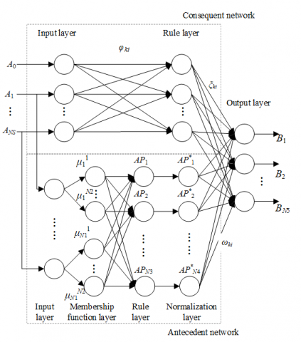
This section mainly introduces the proposed ANN evaluation model. In this paper, the FNN is selected to evaluate the subgrade stability, thanks to its connected structure, self-learning ability, as well as advanced fuzzy thinking and evaluation structure.
Figure 5. The structure of Takagi-Sugeno fuzzy system
Unlike the Mamdani model in which the consequent of fuzzy rules is a fuzzy set, the Takagi-Sugeno fuzzy system, which is based on the linear combination of input variables, is suitable for processing the data on the influencing factors of unstable subgrade deformation. Figure 5 presents the structure of Takagi-Sugeno fuzzy system. Obviously, Takagi-Sugeno fuzzy system has a similar antecedent network as the Mamdani model. The network mainly matches the fuzzy rules of subgrade stability evaluation.
In the fuzzy system, each input layer node is directly connected to the input vector Ai. The number of nodes N1=NS. In addition, the membership function layer computes the membership of Ai relative to the fuzzy set of linguistic variables corresponding to the nodes on each fuzzy layer:
$\mu _{i}^{k}=\exp [-\frac{{{({{A}_{i}}-{{\varphi }_{ik}})}^{2}}}{\gamma _{ik}^{2}}]$ (26)
where, μik is the membership of Ai belonging to the k-th fuzzy set; ϕik is the center of the membership function; γik is the width of the membership function. The number of nodes in that fuzzy layer can be derived from the fuzzy segmentation number vi of Ai:
${{N}_{2}}=\sum\limits_{i=1}^{{{N}_{S}}}{{{v}_{i}}}$ (27)
The rule layer matches the fuzzy rules corresponding to the nodes on each rule layer, and calculates the applicability of each rule by:
$A{{P}_{k}}=\mu _{1}^{{{k}_{1}}}\mu _{2}^{{{k}_{2}}}\cdots \mu _{2}^{{{k}_{{{N}_{S}}}}}$ (28)
where, k1=1, 2, …, v1; k2=1, 2, …, v1; kNS=1, 2, …, vNS. The number of nodes in each rule layer can be calculated by:
${{N}_{3}}=V=\prod\limits_{i=1}^{{{N}_{S}}}{{{v}_{i}}}$ (29)
The number of nodes N4 in the normalization layer is the same that N3 in the rule layer. The normalization layer mainly performs normalization by:
$AP_{k}^{*}=\frac{A{{P}_{k}}}{\sum\limits_{i=1}^{V}{A{{P}_{i}}}}$ (30)
Let ωki be the connection weight between the normalization layer and output layer. Then, the network output can be obtained by:
${{B}_{i}}=\sum\limits_{k=1}^{V}{{{\omega }_{ki}}AP_{k}^{*}}$ (31)
The consequent network of Takagi-Sugeno fuzzy system consists of the following three layers:
The input layer transfers Ai to the rule layer. To provide the consequent of each fuzzy rule with a constant term, the input A1 of the first node was set to 1. Then, the rule layer computes the consequents of the V fuzzy rules represented by V nodes by:
${{z}_{k}}={{\phi }_{k0}}+{{\phi }_{k1}}{{A}_{1}}+\ldots +{{\phi }_{k{{N}_{S}}}}{{A}_{{{N}_{S}}}}$ (32)
Let ξki be the connection weight between the rule layer and the output layer. Then, the network output can be obtained by:
${{B}_{i}}=\sum\limits_{k=1}^{V}{{{\xi }_{ki}}{{z}_{k}}AP_{k}^{*}}\text{ }$ (33)
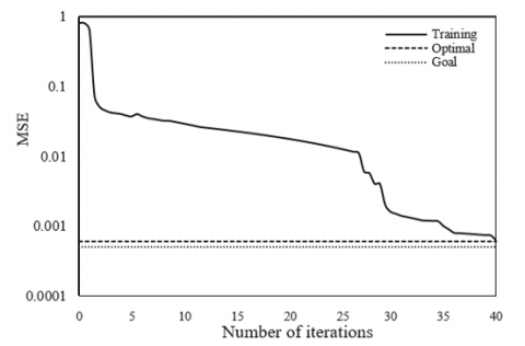
The FNN based on Takagi-Sugeno model was realized on MATLAB. The data on the influencing factors of unstable subgrade deformation in the target highway section were collected from 1,200 monitoring points, and taken as the input of the FNN. Then, the FNN was trained to obtain the highly nonlinear mapping between the influencing factors and the subgrade stability levels. The number of nodes in the membership function layer of the FNN was set to 30 for temperature influence analysis, 38 for moisture influence analysis, and 27 for traffic load influence analysis.
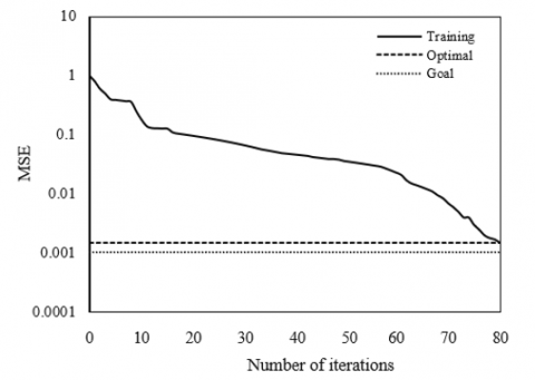
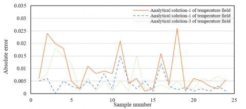
Figure 6 presents the analysis results on temperature influence over subgrade stability. The training error of the FNN is displayed in subgraph (a), and the fluctuation of the error between the actual and trained temperature influences is presented in subgraph (b). It can be seen that the FNN reached the preset training accuracy after around 80 iterations; most analytical solutions of temperature field of the subgrade fit well with the trained values. The error was relatively large at some monitoring points, due to the problem in the deployment of monitoring points. Such an error can be neglected.
(a) Training error
(b) Error fluctuation
Figure 6. The analysis results on temperature influence over subgrade stability
(a) Training error
(b) Error fluctuation
Figure 7. The analysis results on moisture influence over subgrade stability
(a)Training error
(b)Error fluctuation
Figure 8. The analysis results on traffic load influence over subgrade stability
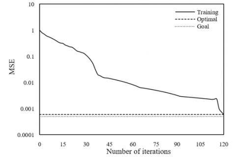
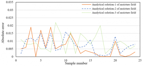
Figure 7 presents the analysis results on moisture influence over subgrade stability. The training error of the FNN is displayed in subgraph (a), and the fluctuation of the error between the actual and trained moisture influences is presented in subgraph (b). It can be seen that the FNN reached the preset training accuracy after around 40 iterations; the analytical solutions of moisture field of the subgrade fit well with the trained values, and the error curve did not fluctuate significantly, an evidence of high training quality.
Figure 8 presents the analysis results on traffic load influence over subgrade stability. The training error of the FNN is displayed in subgraph (a), and the fluctuation of the error between the actual and trained traffic load influences is presented in subgraph (b). It can be seen that the FNN basically reached the preset training accuracy, when the training ended after around 120 iterations; the expected traffic load influence on the subgrade fit well with the trained values, and the training situation was good, despite the large fluctuation of error at a few samples.
In summary, the FNN controlled the training errors of the analytical solutions to temperature field, moisture field, and traffic load within 2.5%, 2.15%, and 5%, respectively. These errors all satisfy the requirements of subgrade engineering.
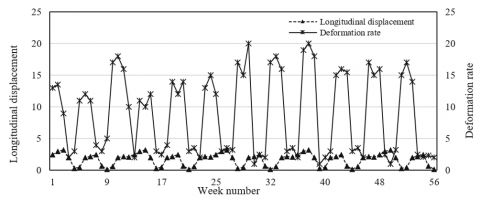
Figure 9 records the annual changes in longitudinal displacement and deformation rate of the subgrade. The curves in the figure intuitively display the unstable deformation of the subgrade and pavement throughout a year, and reflect the degree of uneven deformation of subgrade cross section. It can be seen that the longitudinal displacement and deformation rate of subgrade cross section varied regularly from week to week throughout the year. The deformation rate fell in the range of 0.08%~0.35%, which is smaller than the upper bound (4%) of the deformation rate that ensures driving comfort.
Figure 9. The annual changes in longitudinal displacement and deformation rate of the subgrade
Table 2. The monitored and predicted results on unstable subgrade deformation at different monitoring points
|
Monitoring point Displacement |
1 |
2 |
3 |
4 |
5 |
6 |
7 |
8 |
9 |
10 |
|
Monitored value (mm) |
1.82 |
2.57 |
4.21 |
3.57 |
6.75 |
5.21 |
4.09 |
4.96 |
2.19 |
5.28 |
|
Predicted value (mm) |
1.89 |
2.69 |
4.33 |
3.46 |
6.69 |
5.15 |
3.98 |
4.87 |
2.08 |
5.20 |
|
Relative error |
3.8% |
4.7% |
2.8% |
3.1% |
0.09% |
1.2% |
2.7% |
1.8% |
5% |
1.5% |
As shown in Table 2, among the 10 monitoring points, the largest displacements were observed at the 2nd and 9th points. The two points are located in an uphill section and at a slope inflection point, respectively. The results show that the uphill section and slope inflection point are two stability hazard points. The relative error between monitored and predicted displacements was smaller than 4% at any other point. This means our model is feasible for subgrade stability evaluation, and appliable to actual subgrade engineering.
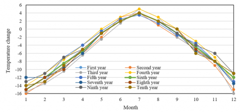
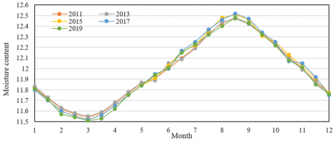
Figure 10 shows the predicted trends of temperature and moisture content at a subgrade monitoring point. The annual trend of mean monthly temperature change at the point is given in subgraph (a), while the moisture content at 1.5m underground at the point is provided in subgraph (b). It can be seen that the predicted analytical solution to temperature field was minimized in January and February, and peaked in July and August; the moisture content in the subgrade followed the same trend with regional rainfall: the valley lasted from February to April, and the peak appeared in August to October. The two trend maps largely overlap each other in the ten years, which meet the actual situation. In this way, the proposed model was proved valid and accurate.
(a) Monthly trend
(b) Annual trend
Figure 10. The predicted trends of temperature and moisture content at a subgrade monitoring point
This paper mainly establishes an ANN-based evaluation model for subgrade stability. Firstly, the influencing factors of subgrade stability, including temperature field, moisture field, and traffic load, were analyzed to obtain the change law of unstable deformation of highway subgrade in special areas. Next, the correlations between input and output characteristic quantities were extracted to optimize the parameter features of subgrade stability, followed by the construction of the nonredundant mapping function between influencing factors of subgrade unstable deformation and the levels of subgrade stability. Finally, an FNN was established for the evaluation of subgrade stability, and proved valid through experiments on the main influencing factors. The experimental results show that our model controlled the relative error between predicted and actual subgrade displacement within 4%, and forecasted the trends of temperature and moisture content in subgrade realistically. Hence, our model is feasible for subgrade stability evaluation, and appliable to actual subgrade engineering.
This work was supported by National Natural Science Foundation of China (51378164); Natural Science Foundation of Heilongjiang (E2016045).
[1] Akimov, S., Kosenko, S., Bogdanovich, S. (2019). Stability of the supporting subgrade on the tracks with heavy train movement. In International Scientific Siberian Transport Forum, 1116: 228-236. https://doi.org/10.1007/978-3-030-37919-3_22
[2] Suwantara, I.K., Wardani, S.P.R., Priastiwi, Y.A. (2019). Expansive clay soil stabilization using white soil material and sulfuric acid solution (H2SO4) For subgrade in Godong Area-Grobogan District. In IOP Conference Series: Earth and Environmental Science, 328(1): 012022. https://doi.org/10.1088/1755-1315/328/1/012022
[3] Wysocki, G., Ksi, B., Kucz, M. (2017). The influence of a low bearing subgrade on the stability of a shared street (woonerf) foundation. Procedia Engineering, 172: 1252-1260. https://doi.org/10.1016/j.proeng.2017.02.147
[4] Stoyanovich, G.M., Pupatenko, V.V., Maleev, D.Y., Zmeev, K.V. (2017). Solution of the problem of providing railway track stability in joint sections between railroad facilities and subgrade. Procedia Engineering, 189: 587-592. https://doi.org/10.1016/j.proeng.2017.05.093
[5] Adeyanju, E., Okeke, C.A., Akinwumi, I., Busari, A. (2020). Subgrade stabilization using rice husk ash-based geopolymer (GRHA) and cement kiln dust (CKD). Case Studies in Construction Materials, 13: e00388. https://doi.org/10.1016/j.cscm.2020.e00388
[6] Rabab’ah, S., Al Hattamleh, O., Aldeeky, H., Aljarrah, M.M., Al_Qablan, H.A. (2020). Resilient response and permanent strain of subgrade soil stabilized with byproduct recycled steel and cementitious materials. Journal of Materials in Civil Engineering, 32(6): 04020139.
[7] Buslov, A., Margolin, V. (2017). The interaction of piles in double-row pile retaining walls in the stabilization of the subgrade. In Energy Management of Municipal Transportation Facilities and Transport, 692: 769-775. https://doi.org/10.1007/978-3-319-70987-1_81
[8] Akpinar, M.V., Pancar, E.B., Şengül, E., Aslan, H. (2018). Pavement subgrade stabilization with lime and cellular confinement system. The Baltic Journal of Road and Bridge Engineering, 13(2): 87-93. https://doi.org/10.7250/bjrbe.2018-13.402
[9] Ramli, R., Yahaya, N.N., Bakar, N.N.A.A., Dollah, Z., Idrus, J., Abdullah, N.H.H. (2019). Effectiveness of crushed coconut shell and eggshell powder to act as subgrade stabilizer. In Journal of Physics: Conference Series, 1349(1): 012076. https://doi.org/10.1088/1742-6596/1349/1/012076
[10] Tavakol, M., Hossain, M., Tucker-Kulesza, S.E. (2019). Subgrade soil stabilization using low-quality recycled concrete aggregate. In Geo-Congress 2019: Geotechnical Materials, Modeling, and Testing, pp. 235-244.
[11] Chibuzor, O.K., Van Duc, B. (2018). Predicting subgrade stiffness of nanostructured palm bunch ash stabilized lateritic soil for transport geotechnics purposes. Journal of GeoEngineering, 13(1): 167-175. https://doi.org/10.6310/jog.2018.13(1).3
[12] Nagrale, P.P., Patil, A.P. (2017). Improvement in engineering properties of subgrade soil due to stabilization and its effect on pavement response. Geomechanics and Engineering, 12(2): 257-267. https://doi.org/10.12989/gae.2017.12.2.257
[13] Kovalchuk, V., Sysyn, M., Nabochenko, O., Pentsak, A., Voznyak, O., Kinter, S. (2019). Stability of the railway subgrade under condition of its elements damage and severe environment. In MATEC Web of Conferences, 294: 03017. https://doi.org/10.1051/matecconf/201929403017
[14] Behnood, A., Olek, J. (2020). Full-scale laboratory evaluation of the effectiveness of subgrade soil stabilization practices for Portland cement concrete pavements patching applications. Transportation Research Record, 2674(5): 465-474. https://doi.org/10.1177/0361198120916476
[15] Azizan, F.A., Marhami, N.S., Abd Rahman, Z., Arshad, A.K., Ismail, M.K.A. (2020). Evaluation of the use of tiles waste in stabilization of subgrade layer with rice husk ash as an activator agent. In IOP Conference Series: Earth and Environmental Science, 476(1): 012042. https://doi.org/10.1088/1755-1315/476/1/012042
[16] Neupane, M., Han, J., Parsons, R.L. (2020). Experimental and analytical evaluations of mechanically-stabilized layers with geogrid over weak subgrade under static loading. In Geo-Congress 2020: Engineering, Monitoring, and Management of Geotechnical Infrastructure, pp. 597-606.
[17] Mishra, S., Sachdeva, S.N., Manocha, R. (2019). Subgrade soil stabilization using stone dust and coarse aggregate: A cost effective approach. International Journal of Geosynthetics and Ground Engineering, 5(3): 20. https://doi.org/10.1007/s40891-019-0171-0
[18] Apriyanti, Y., Fahriani, F., Fauzan, H. (2019). Use of gypsum waste and tin tailings as stabilization materials for clay to improve quality of subgrade. In IOP Conference Series: Earth and Environmental Science, 353(1): 012042. https://doi.org/10.1088/1755-1315/353/1/012042
[19] Kumar, V., Panwar, R.S. (2019). Mitigation of greenhouse gas emissions by fly ash stabilization and sisal fibre reinforcement of clay subgrade for road construction. In IOP Conference Series: Earth and Environmental Science, 219(1): 012020. https://doi.org/10.1088/1755-1315/219/1/012020
[20] Ikeagwuani, C.C., Nwonu, D.C. (2019). Resilient modulus of lime-bamboo ash stabilized subgrade soil with different compactive energy. Geotechnical and Geological Engineering, 37(4): 3557-3565. https://doi.org/10.1007/s10706-019-00849-6
[21] Wheeler, L.N., Take, W.A., Hoult, N.A. (2017). Performance assessment of peat rail subgrade before and after mass stabilization. Canadian Geotechnical Journal, 54(5): 674-689. https://doi.org/10.1139/cgj-2016-0256
[22] Daud, N.N., Jalil, F.N.A., Celik, S., Albayrak, Z.N.K. (2019). The important aspects of subgrade stabilization for road construction. In IOP Conference Series: Materials Science and Engineering, 512(1): 012005. https://doi.org/10.1088/1757-899X/512/1/012005
[23] Yadav, A.K., Gaurav, K., Kishor, R., Suman, S.K. (2017). Stabilization of alluvial soil for subgrade using rice husk ash, sugarcane bagasse ash and cow dung ash for rural roads. International Journal of Pavement Research and Technology, 10(3): 254-261. https://doi.org/10.1016/j.ijprt.2017.02.001
[24] Aneke, I.F., Hassan, M.M., Moubarak, A. (2019). Shear strength behavior of stabilized unsaturated expansive subgrade soils for highway backfill. In Bituminous Mixtures and Pavements VII: Proceedings of the 7th International Conference' Bituminous Mixtures and Pavements'(7ICONFBMP), June 12-14, 2019, Thessaloniki, Greece, 111.
[25] Ikeagwuani, C.C., Obeta, I.N., Agunwamba, J.C. (2019). Stabilization of black cotton soil subgrade using sawdust ash and lime. Soils and Foundations, 59(1): 162-175. https://doi.org/10.1016/j.sandf.2018.10.004