
Kullawut Karoonwattana | Harnpon Phungrassami | Phairat Usubharatana*
© 2026 The authors. This article is published by IIETA and is licensed under the CC BY 4.0 license (http://creativecommons.org/licenses/by/4.0/).
OPEN ACCESS
This study evaluates greenhouse gas (GHG) emissions from fossil fuel combustion associated with paper products in Thailand using an input–output (IO) analysis. Fuel consumption data were obtained from Thailand’s Energy Efficiency Situation and Energy Balance reports for 2015 and 2021 and integrated with IO tables to estimate economy-wide total GHG emissions across 14 aggregated sectors and emissions associated with paper products from a final-demand-based perspective. The results show that total GHG emissions associated with paper products increased from 0.88 Mt CO₂e in 2015 to 1.61 Mt CO₂e in 2021, while emission intensity increased from 0.1449 t CO₂e/t to 0.2692 t CO₂e/t. The temporal comparison was conducted using monetary IO data harmonized to a common 2015 price basis. The observed changes reflect variations in final demand, production structure, and emission coefficients, which were subsequently examined using additive structural decomposition analysis (SDA) based on the average of two polar decompositions. The SDA attributed +3.375 Mt CO₂e to changes in final demand, −14.405 Mt CO₂e to changes in the Leontief-inverse production structure, and +14.468 Mt CO₂e to changes in emission coefficients, yielding a net increase of 3.438 Mt CO₂e. These results demonstrate that the net emission change resulted from substantial offsetting effects rather than from a single dominant driver. The estimated emission intensities are compared with national Carbon Footprint of Products (CFP) benchmarks as contextual references, considering differences in system boundaries, temporal coverage, product composition, and allocation procedures. These findings highlight the importance of considering demand-side changes, intersectoral production requirements, and fossil-fuel emission coefficients jointly when developing decarbonization strategies in Thailand.
additive structural decomposition analysis, emission intensity, fossil fuel combustion, greenhouse gas emissions, input–output analysis, paper products, Thailand
The increasing concentration of greenhouse gases (GHGs) in the atmosphere remains one of the most critical global challenges. This trend is largely driven by continued reliance on fossil fuel combustion for energy production and industrial activities. The energy sector accounts for the largest share of global emissions, highlighting the need for robust and consistent assessment frameworks to support mitigation strategies and sustainable development pathways [1].
Paper and paper products play an essential role in modern economies, particularly in packaging, communication, and hygiene applications. Global consumption averages approximately 55–60 kg per capita per year, although this varies significantly across regions [2]. In developed economies, demand has declined slightly due to digital substitution. In contrast, emerging economies continue to experience growth, mainly driven by packaging demand.
In Thailand, the pulp, paper, and paper products industry serves both domestic and international markets. In 2021, the production indices of pulp, paper, and packaging increased by 3.57%, 4.07%, and 0.62%, respectively, while the export value of pulp, paper, and print media was estimated at USD 2,401.02 million [3]. The sector is closely linked with upstream industries such as raw material supply, energy production, and transportation. National statistics indicate that industrial activities in Thailand rely heavily on fossil fuels, including petroleum products, natural gas, and coal [4]. As a result, GHG emissions associated with paper products extend beyond direct production. They also include indirect emissions embedded in upstream supply chains [2].
Life Cycle Assessment (LCA), a bottom-up approach based on process-level data, has been widely used to evaluate environmental impacts. However, LCA is often limited by data availability and system boundary constraints, particularly in developing country contexts [5]. In contrast, Input–output Analysis (IOA), a top-down economic framework developed by Leontief [6], captures interconnections between economic sectors and enables the estimation of both direct and indirect emissions across supply chains [6, 7]. By integrating IOA with energy-based emission data, it is possible to assess emissions driven by final demand in a more comprehensive and system-wide manner [7].
Despite these methodological advances, existing studies rarely isolate GHG emissions arising specifically from fossil fuel combustion within input–output (IO)-based frameworks, particularly in sector-specific applications. Moreover, limited research has systematically examined temporal changes in emissions using consistent methodologies across multiple years. This limitation is particularly significant for Thailand, where structural changes in economic activities, energy consumption patterns, and industrial development between 2015 and 2021 may substantially influence emission profiles. A consistent and comparative analytical framework is therefore required to robustly capture the underlying structural and temporal dynamics.
Accordingly, this study aims to quantify the total GHG emissions associated with paper products in Thailand by applying an integrated IO and fossil fuel combustion approach. The analysis focuses on two reference years, 2015 and 2021, to evaluate changes in total GHG emissions and economy-wide structural dynamics across 14 aggregated industrial sectors, while emission intensity is assessed specifically for paper products.
This study makes three key contributions. First, it develops a consistent framework for estimating GHG emissions based explicitly on fossil fuel combustion within an IO structure, ensuring alignment with national energy statistics. Second, it captures both direct and indirect GHG emissions arising from fossil fuel combustion across the domestic intersectoral production system, enabling a more explicit representation of energy-related emission linkages associated with paper products within Thailand. Third, it compares IO-based emission intensity for paper products with national carbon footprint benchmarks provided by the Thailand Greenhouse Gas Management Organization (TGO), thereby strengthening the sector-specific policy relevance of the results.
The results provide critical insights into emission hotspots, structural drivers, and methodological differences, with particular emphasis on total GHG emissions and emission intensity for paper products in Thailand. By highlighting sector-specific emission characteristics and supply chain linkages driven by fossil fuel consumption, the findings support the development of more targeted and policy-relevant mitigation strategies for paper products industry, while also contributing to broader efforts toward sustainable development and low-carbon transition.
2.1 Study framework and data sources
This study adopts an IO-based environmental assessment framework to quantify GHG emissions from fossil fuel combustion across economic sectors in Thailand, with a comparative analysis between 2015 and 2021 [6, 7]. The IO framework has been widely applied in environmental and energy studies to capture intersectoral dependencies and embodied emissions across supply chains, particularly in national-scale assessments [8, 9]. Unlike process-based approaches, IO models provide a comprehensive representation of indirect emissions, which are often underestimated in sector-specific analyses [5, 10]. Rather than relying on a fully integrated environmentally extended input–output (EEIO) database, a customized framework is developed by integrating national IO tables with sectoral energy consumption data and emission factors. This hybridized approach has been shown to improve consistency between economic and environmental datasets while maintaining transparency in emission estimation [7, 11].
The analytical procedure consists of four main steps: (i) estimating sectoral direct emissions based on fossil fuel consumption, (ii) conducting a comparative structural analysis to examine the key drivers of emission changes between 2015 and 2021, (iii) incorporating emission coefficients into the IO framework to estimate total emissions, and (iv) deriving emission intensity indicators.
Energy consumption data were obtained from Thailand Energy Efficiency Situation and Energy Balance reports for 2015 and 2021 [4, 12, 13]. Emission factors were sourced from TGO [14], and economic data were derived from Thailand’s IO tables compiled by the Office of the National Economic and Social Development Council [15].
To ensure comparability between the 2015 and 2021 monetary IO data, all monetary variables used for the temporal comparison were expressed at constant 2015 prices. The 2015 IO table was retained as the base-year price structure, while the 2021 monetary flows were deflated using the closest available producer price indices (PPI) from the Trade Policy and Strategy Office (TPSO), Ministry of Commerce, Thailand. The PPI series was selected according to the Classification of Products by Activity (CPA), with 2015 as the base year (2015 = 100) and 2021 as the target year. The price harmonization was applied consistently to final demand, intermediate transactions, gross output, and the corresponding IO coefficients used in the 2021 model.
Because the monetary IO tables for 2015 and 2021 are expressed in nominal/current prices, the 2021 IO data were converted to a common 2015 constant-price basis before conducting the temporal comparison. Sector-matched price deflation was performed using the closest available producer or service price indices from the TPSO, with 2015 = 100 as the reference price basis. The price harmonization was applied consistently to intermediate transactions, total output, and final demand. The technical coefficient matrix and Leontief inverse for 2021 were subsequently recalculated using the price-harmonized IO data.
2.2 System boundary and scope definition
The system boundary of this study is defined to include GHG emissions arising exclusively from fossil fuel combustion within domestic economic activities in Thailand. This definition follows established guidelines for energy-related emissions accounting and ensures consistency with international reporting standards [16, 17].
The analysis encompasses all economic sectors and fossil fuel types considered in this study, with detailed classification and data harmonization procedures provided in Section 2.3 to ensure consistency between energy consumption data and the IO framework.
Within this boundary, direct fossil-fuel combustion emissions are estimated for all 14 economic sectors based on sectoral fuel consumption data, including Public Utilities (PubU) and Transport and Communication (T&C). These sectoral emissions are subsequently propagated through intersectoral linkages in the domestic IO framework to capture indirect emissions associated with final demand. Accordingly, fossil-fuel combustion emissions from upstream electricity generation and transportation activities are included when they are represented as domestic sectoral production requirements in the IO system. Imported intermediate inputs and imported final goods are not separately modeled by foreign producing sectors; therefore, fossil-fuel emissions embodied in foreign upstream production are outside the system boundary. The resulting estimates represent emissions associated with domestic production requirements within Thailand rather than the full global supply chain [8, 16].
2.3 Data sources and integration
This study integrates three primary datasets: (i) sectoral energy consumption, (ii) emission factors, and (iii) economic IO tables, to construct a consistent analytical framework for estimating GHG emissions.
Energy consumption data were obtained from Thailand’s national energy statistics [4, 12, 13], which provide detailed fossil fuel consumption across sectors and fuel types. Emission factors were sourced from TGO [14], ensuring consistency with national GHG accounting practices. Economic data were derived from IO tables compiled by NESDC [15].
To ensure consistency between the economic and energy datasets, the original 16-sector classification of the IO tables was aggregated into the 14-sector classification used in the national energy statistics. Specifically, the “Other” and “Unclassified” sectors were combined into “Unclassified (UnCl)”, while the “Trade” and “Services” sectors were combined into “Trade and Services (T&S)”. This sector aggregation established a consistent sector classification between the IO tables and the national fuel consumption data.
Following this sector aggregation, fossil fuel consumption data were mapped to the corresponding IO sectors using a sector–fuel concordance. The fuel types include liquefied petroleum gas (LPG), kerosene, premium gasoline, regular gasoline, high-speed diesel, low-speed diesel, fuel oil, natural gas, and coal, consistent with the national energy statistics. The resulting sector–fuel mapping is summarized in Table 1, based on observed fuel consumption in 2015 and 2021 [4, 12, 13].
The integration of physical energy data with monetary IO tables is a critical step in environmentally extended IO analysis and has been widely applied in previous studies [7, 9, 18]. This approach ensures consistency between physical energy flows and economic transactions while maintaining methodological transparency.
For temporal comparison, the monetary IO data were harmonized to constant 2015 prices. The 2021 price adjustment used sector-matched price deflators derived from the closest available TPSO producer/service price indices classified according to the CPA. This treatment was necessary because directly corresponding price indices were not available for all aggregated IO sectors [19-21].
Table 1. Sector-fuel mapping framework used in this study based on the harmonized 14-sector classification
|
Sector |
LPG |
Kerosene |
Premium Gasoline |
Regular Gasoline |
High-Speed Diesel |
Low-Speed Diesel |
Fuel Oil |
NG |
Coal |
|
Agriculture (Agr) |
– |
– |
✓ |
✓ |
✓ |
– |
– |
– |
– |
|
Mining (Min) |
– |
– |
|
– |
✓ |
– |
– |
– |
– |
|
Food and Beverage (F&B) |
✓ |
✓ |
✓ |
✓ |
✓ |
– |
✓ |
✓ |
✓ |
|
Textiles (Tex) |
✓ |
– |
✓ |
✓ |
✓ |
– |
✓ |
✓ |
✓ |
|
Saw Mills and Wood Products (S&W) |
✓ |
– |
|
✓ |
✓ |
– |
✓ |
✓ |
– |
|
Paper (Pap) |
✓ |
✓ |
✓ |
✓ |
✓ |
– |
✓ |
✓ |
✓ |
|
Chemicals (Chem) |
✓ |
✓ |
✓ |
✓ |
✓ |
– |
✓ |
✓ |
✓ |
|
Non-metallic (NonM) |
✓ |
✓ |
✓ |
– |
✓ |
– |
✓ |
✓ |
✓ |
|
Metal (Met) |
✓ |
✓ |
✓ |
✓ |
✓ |
– |
✓ |
✓ |
✓ |
|
Public Utilities (PubU) |
– |
– |
– |
– |
✓ |
– |
✓ |
✓ |
✓ |
|
Construction (Cstr) |
– |
– |
– |
– |
✓ |
– |
✓ |
– |
– |
|
Transport and Communication (T&C) |
✓ |
– |
✓ |
✓ |
✓ |
✓ |
✓ |
✓ |
– |
|
Trade and Services (T&S) |
✓ |
– |
|
|
|
– |
– |
✓ |
– |
|
Unclassified (UnCl) |
✓ |
– |
✓ |
✓ |
✓ |
– |
✓ |
✓ |
✓ |
Note: ✓ indicates the presence of fuel consumption based on national energy statistics (2015 and 2021). LPG = liquefied petroleum gas; NG = natural gas.
2.4 Input–output model formulation and price harmonization
The intersectoral transaction matrix $Z$ is derived from the IO tables and represents the monetary flows between economic sectors [7]. This matrix forms the basis for describing the interdependencies of production activities within the economy and has been widely applied in economic and environmental system analysis [8, 22].
The technical coefficient matrix $A$ is calculated by normalizing intersectoral transactions by total sectoral output. Each element $A_{i j}$ represents the input required from sector $i$ to produce one unit of output in sector $j$, thereby reflecting the production structure of the economy [7, 23]. In practical terms, this matrix quantifies how production in one sector depends on inputs from other sectors and is fundamental to IO modeling.
The technical coefficient matrix is defined as:
$A_{i j}=\frac{Z_{i j}}{x_j}$ (1)
where, $Z_{i j}$ represents the monetary flow from sector $i$ to sector $j$, and $x_j$ is the total output of sector $j$ [7].
The total output required to satisfy final demand is expressed as:
$x=(I-A)^{-1} y$ (2)
where, $I$ is the identity matrix, and $y$ is the final demand vector. The Leontief inverse matrix $(I-A)^{-1}$ represents the total (direct and indirect) production requirements across all sectors and forms the core analytical component for tracing supply chain effects [7, 9, 22].
Price harmonization of monetary IO data: to enable a meaningful comparison between 2015 and 2021, the 2015 IO table was retained as the reference price basis, while the 2021 monetary transactions were converted to 2015 constant prices using sector-matched price indices from the TPSO. Let $P_i$ denote the 2021 price index for sector $i$, with 2015 = 100. The corresponding deflation factor was calculated as $P_i / 100$, and the 2021 monetary values were converted to 2015 constant prices by dividing the corresponding values by this factor. As shown in Table 2, sector-specific price indices were assigned to the aggregated IO sectors according to the closest available TPSO price categories. For the Paper sector, the matched Paper and Paper Products price index was 104.3, indicating that the corresponding 2021 monetary values were deflated by a factor of 1.043 . For the Rubber, Chemical sector, which combines petroleum refining, chemical, and rubber and plastic activities, an index of 104.5 was applied based on the available matched price categories. For sectors without a directly corresponding TPSO price category, including PubU, Construction, Transportation, and T\&S, the common All (Proxy) index of 102.3 was applied. The Unclassified sector was assigned an index of 100.0, implying no price adjustment relative to the 2015 reference basis. The resulting sector-matched deflators were consistently applied to the intermediate transaction matrix, total output, and final demand vector to express the 2021 IO data in 2015 constant prices before conducting the temporal comparison and structural decomposition analysis (SDA) [19-21].
Table 2. Sector-matched price deflators used to convert the 2021 input–output (IO) data to 2015 constant prices
|
IO Sector |
TPSO Price Category |
2021 Index (2015 = 100) |
|
Agriculture (Agr) |
Agricultural and Fishery Products |
104.5 |
|
Mining (Min) |
Mining Products |
97.7 |
|
Food and Beverage (F&B) |
Food Products |
103.0 |
|
Textiles (Tex) |
Textiles |
99.3 |
|
Saw Mills and Wood Products (S&W) |
Wood and Wood Products |
99.7 |
|
Paper (Pap) |
Paper and Paper Products |
104.3 |
|
Chemicals (Chem) |
Average Petroleum Refining Products, Chemicals and Chemical Products, Rubber and Plastic Products |
104.5 |
|
Non-metallic (NonM) |
Non-Metallic Mineral Products |
100.5 |
|
Metal (Met) |
Basic Metals |
109.0 |
|
Public Utilities (PubU) |
All (Proxy) |
102.3 |
|
Construction (Cstr) |
All (Proxy) |
102.3 |
|
Transport and Communication (T&C) |
All (Proxy) |
102.3 |
|
Trade and Services (T&S) |
All (Proxy) |
102.3 |
|
Unclassified (UnCl) |
Other Products Not Elsewhere Classified |
100.0 |
Note: TPSO = Trade Policy and Strategy Office.
2.5 Estimation of greenhouse gas emissions from fossil fuel combustion
Direct GHG emissions from fossil fuel combustion are estimated for each sector using fuel consumption data and corresponding emission factors. Fuel consumption data were converted from the reporting units used in the national energy statistics to the units required by the corresponding emission factors using the fuel-specific conversion factors documented in the calculation files. Fuel consumption, denoted as $F_{i, f}$, represents the amount of fuel type $f$ consumed by sector $i$. The emission factor, denoted as $E F_f$, represents the amount of emissions generated per unit of fuel consumed. The resulting emissions are expressed in kg $\mathrm{CO}_2$ and represent sectoral direct emissions associated with fossil fuel combustion. The use of fuel-specific emission factors enables differentiation across fuel types with varying carbon intensities, thereby improving the accuracy and consistency of emission estimation in sectoral analysis [14]. This formulation is widely applied in energy and environmental studies to quantify emissions at the sector level prior to integration into IO models. The direct emissions are calculated as:
$E_i=\sum_f\left(F_{i, f} \times E F_f\right)$ (3)
where, $E_i$ represents total direct GHG emissions from sector $i$, aggregated across all fuel types $f$. These emissions represent direct fossil-fuel combustion emissions occurring within each sector and are distinguished from final-demand-based embodied emissions calculated subsequently through the IO framework.
2.6 Construction of emission coefficients
Emission coefficients are calculated to integrate environmental information into the IO framework. For each sector $i$, the emission coefficient is defined as the ratio of direct GHG emissions to total sectoral output, as expressed in Eq. (4). Specifically, $e_i$ represents the emission coefficient, $E_i$ denotes direct GHG emissions from fossil fuel combustion in sector $i$, and $x_i$ is the total economic output of that sector.
$e_i=\frac{E_i}{x_i}$ (4)
The resulting coefficient $e_i$ represents the amount of emissions generated per unit of economic output (kg CO₂e/THB). These coefficients represent emissions per unit of economic output and are commonly used in environmentally extended IO models [7, 9]. They enable the integration of environmental data with economic systems and facilitate embodied emission analysis [11, 18]. The emission coefficient therefore represents the direct fossil-fuel combustion emissions per unit of sectoral economic output and serves as the environmental extension coefficient for calculating final-demand-based embodied emissions in the IO framework.
For 2021, the emission coefficient was recalculated using constant-price sectoral output. Physical direct GHG emissions $E_i$, derived from fuel consumption and emission factors, were not deflated because they represent physical emission quantities.
2.7 Input–output-based embodied emissions
Total GHG emissions associated with economic activities are estimated by integrating emission coefficients with the IO framework:
$C=e(I-A)^{-1} y=e L y$ (5)
where, $C$ represents total GHG emissions, $e$ is the vector of emission coefficients, and $L=$ $(I-A)^{-1}$ is the Leontief inverse matrix, and $y$ is the final-demand vector. The formulation captures the direct and indirect GHG emissions required to satisfy final demand through the modeled domestic production system [7, 22]. The resulting emissions are therefore interpreted as final-demand-based embodied emissions rather than direct production emissions, which are calculated separately from sectoral fossil fuel consumption in Section 2.5.
For the economy-wide assessment, $y$ contains the final-demand values of all 14 sectors, and $C=e L y$ represents the total GHG emissions embodied in aggregate final demand. For a specific sector $j$, sector-specific embodied emissions are obtained by constructing a sector-specific final-demand vector $y_j$, in which the final-demand value of sector $j$ is retained and the final-demand values of all other sectors are set to zero. The corresponding sector-specific embodied emissions are calculated as
$C_j=e L y_j$ (6)
where, $C_j$ represents the GHG emissions embodied in the final demand of sector $j$.
For paper products, the paper-specific final-demand vector is defined as
$y_{\text {Pap }}=s_{\text {Pap}} y_{\text {Pap}}$ (7)
where, $s_{\text {Pap}}$ is a $14 \times 1$ sector-selection vector with a value of 1 for the Paper (Pap) sector and 0 for all other sectors, and $y_{\text {Pap}}$ is the final-demand value of the Paper sector. Thus, $y_{\text {Pap}}$ contains the Paper-sector final demand while all other sectoral final-demand components are set to zero. The paper-specific embodied GHG emissions are subsequently calculated as
$C_{\text {Pap}}=e L y_{\text {Pap}}$ (8)
This result represents the direct and indirect GHG emissions embodied in the domestic production requirements associated with paper-sector final demand. Because the model is based on a domestic single-region IO table, imported intermediate inputs are not traced to their foreign producing sectors, and their upstream fossil-fuel emissions are therefore not included in the estimated embodied emissions. The paper-specific embodied-emission result should be distinguished from the final-demand effect obtained from the SDA. Specifically, $C_{\text {Pap}}$ represents the total embodied emissions associated with paper-sector final demand, whereas $\Delta C_y$ represents the economy-wide contribution of changes in final demand to the change in total GHG emissions between 2015 and 2021.
For the 2021 constant-price framework, the total economy-wide emissions were calculated using the price-harmonized variables as $C_{2021}=e_{2021}^{C P} L_{2021}^{C P} y_{2021}^{C P}$, where the emission coefficient, Leontief inverse, and final-demand vector were consistently derived from the price-harmonized IO framework.
2.8 Emission intensity analysis
Emission intensity is defined as the amount of GHG emissions generated per unit of production output and is used to assess the carbon efficiency of production systems. For paper products, emission intensity is calculated as the ratio of paper-specific embodied GHG emissions, obtained from the paper final-demand vector, to the corresponding paper-product production volume, as expressed in Eq. (9). The production volume represents the total output of paper products and excludes pulp production.
$E I_{\text {Pap}}=\frac{C_{\text {Pap}}}{Q_{\text {Pap}}}$ (9)
Specifically, $E I_{\text {Pap}}$ represents the emission intensity of paper products, $C_{\text {Pap}}$ denotes the GHG emissions embodied in the final demand of the Paper sector and $Q_{\text {Pap}}$ denotes the corresponding paper-product production volume.
The resulting emission intensity is expressed in units of t CO₂e per tonne of product (t CO₂e/t) and reflects the overall carbon efficiency of the production system. Emission intensity is a key indicator for evaluating carbon efficiency and is widely used in environmental performance assessment [24, 25]. It enables benchmarking across sectors and comparison with national standards [3, 14].
2.9 Temporal comparison (2015 and 2021) and structural decomposition analysis
A comparative analysis is conducted to examine changes in emissions between 2015 and 2021. This approach is widely used in SDA to identify key drivers of emission changes [8, 26]. By maintaining a consistent framework, the analysis enables robust evaluation of demand, structural, and technological effects [7, 26].
A comparative analysis was conducted to examine changes in GHG emissions between 2015 and 2021 using a common price basis. The 2015 IO data were retained at the reference price basis, while the 2021 monetary IO data were harmonized to 2015 constant prices using sector-matched price deflators.
The temporal comparison between 2015 and 2021 was conducted using a common 2015 constant-price basis. The 2015 IO table was retained as the reference price structure, while the 2021 monetary IO data were harmonized using sector-matched producer or service price deflators derived from the closest available TPSO price indices. The price-harmonized 2021 intermediate transactions, total output, and final demand were then used to recalculate the technical coefficient matrix and the Leontief inverse. Accordingly, monetary changes in final demand between the two years are interpreted on a constant-price basis rather than as changes in current-price values [20, 21].
To identify the determinants of the change in total GHG emissions, an additive SDA was applied to the IO identity $C=e L y$. Let superscript 0 denote 2015 and superscript 1 denote 2021 after price harmonization. The decomposition separates the observed change in total emissions into emission-coefficient, Leontief-inverse (production-structure), and final-demand effects. Because SDA can yield multiple equivalent decompositions depending on the ordering of factors, the present study uses the average of the two polar decompositions, a conventional approach that reduces dependence on a single factor-ordering scheme [11, 26, 27].
$C^t=e^t L^t y^t$ (10)
$\Delta C=C^1-C^0=e^1 L^1 y^1-e^0 L^0 y^0$ (11)
$\Delta C^e=\frac{1}{2} \Delta e\left(L^1 y^1+L^0 y^0\right)$ (12)
$\Delta C^L=\frac{1}{2}\left[e^1 \Delta L y^0+e^0 \Delta L y^1\right]$ (13)
$\Delta C^y=\frac{1}{2}\left[e^1 L^1 \Delta y+e^0 L^0 \Delta y\right]$ (14)
$\Delta C^e+\Delta C^L+\Delta C^y=\Delta C$ (15)
$\Delta e=e^1-e^0, \Delta L=L^1-L^0, \Delta y=y^1-y^0$ (16)
2.10 Uncertainty and limitations
The IO-based emission intensity is compared with national benchmark values derived from the Carbon Footprint of Products (CFP) database developed by TGO. The comparison is used solely as a contextual benchmark for interpreting the magnitude of the IO-based estimate rather than as a formal validation of the IO model.
Differences between the IO-based estimates and the CFP benchmark may arise from differences in temporal coverage, product composition, allocation procedures, system boundaries, and sectoral aggregation. The IO approach represents a top-down economic framework that captures emissions associated with intersectoral production linkages, whereas the CFP benchmark represents product-level emission factors developed under the TGO CFP assessment framework. Therefore, the two estimates are not considered directly equivalent measures, and their quantitative difference is not interpreted as evidence of model validity or invalidity.
The analysis is limited to GHG emissions from fossil fuel combustion and excludes other emission sources such as industrial process emissions, agriculture, land-use change, and waste management, consistent with IPCC guidelines [16, 17]. This restriction ensures methodological consistency but may lead to partial representation of total sectoral emissions.
Additional uncertainties arise from the use of IO tables, sectoral aggregation, and estimated production data. These uncertainties are inherent in IO-based environmental assessments and have been widely discussed in the literature, particularly in the context of multi-region input–output (MRIO) models applied to national carbon footprint analysis [11, 28].
While such uncertainties may influence the magnitude of estimated results, previous studies demonstrate that IO-based approaches remain robust for macro-level analysis and comparative assessments, especially when consistent datasets and methodological frameworks are applied [11, 28].
3.1 Overview of total greenhouse gas emissions
3.1.1 Changes in total greenhouse gas emissions
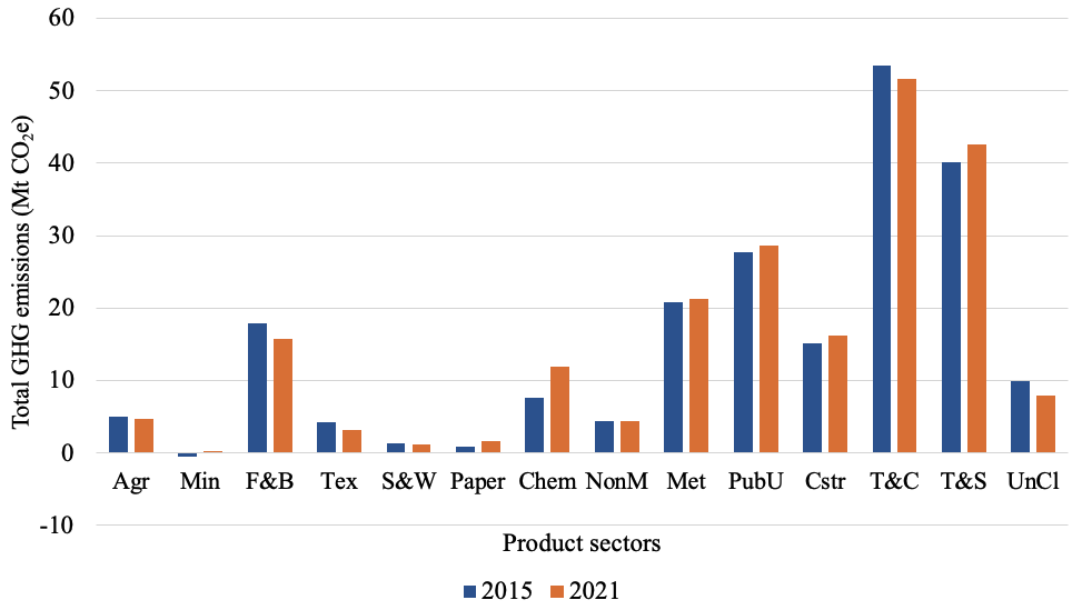
This section presents a comparative analysis of total GHG emissions in Thailand using an IO framework, focusing on structural changes between 2015 and 2021. As shown in Figure 1, total GHG emissions increased from 207.97 Mt CO₂e in 2015 to 211.41 Mt CO₂e in 2021, representing a net increase of 3.438 Mt CO₂e (approximately 1.65%). The 2021 monetary IO framework used in the calculation was harmonized to the 2015 price basis. The net change is subsequently decomposed in Sections 3.1.3–3.1.5 into final-demand, Leontief-inverse, and emission-coefficient effects.
At the sectoral level, PubU remained the largest contributor, with emissions rising slightly from 27.66 Mt CO₂e to 28.66 Mt CO₂e, accounting for approximately 13.3–13.6% of total emissions. Similarly, the T&C and the T&S sectors continued to dominate the emission structure, collectively representing nearly half of total emissions in both years. These sectors are strongly associated with final-demand-driven activities and exhibit extensive intersectoral linkages within the economy.
Notably, emissions embodied in paper products increased substantially, rising from 0.88 Mt CO₂e in 2015 to 1.61 Mt CO₂e in 2021, corresponding to an increase of approximately 83%. This growth significantly exceeds the overall emission trend and indicates a shift in underlying final demand and supply chain structures. In contrast, several traditional manufacturing sectors, such as Food and Beverage (F&B) and Textiles (Tex), showed declining emission contributions, suggesting improvements in production efficiency or a contraction in sectoral activity.
Overall, the relatively small net increase in aggregate emissions masks substantially larger offsetting structural effects. The SDA results reported below quantify these offsetting contributions and provide a more rigorous basis for interpreting the change than a comparison of sector totals alone.
3.1.2 Direct and indirect greenhouse gas emissions associated with paper products
To further clarify the supply-chain contribution of paper products, the total GHG emissions associated with paper-sector final demand were examined in terms of direct and indirect contributions. Direct emissions represent emissions generated within the Paper sector, while indirect emissions represent emissions embodied in upstream intersectoral production requirements captured by the Leontief-based IO framework. As shown in Table 3, total GHG emissions associated with paper products increased from 0.88 Mt CO₂e in 2015 to 1.61 Mt CO₂e in 2021. The results show that both direct and indirect emissions contributed to the total, demonstrating that the GHG emissions associated with paper products extend beyond the Paper sector through upstream supply-chain linkages.
Table 3. Direct and indirect greenhouse gas (GHG) emissions associated with paper products
|
Item |
2015 |
2021 |
|
Total GHG emissions |
0.88 Mt CO₂e |
1.61 Mt CO₂e |
|
Direct emissions |
0.57 Mt CO₂e |
1.18 Mt CO₂e |
|
Indirect emissions |
0.30 Mt CO₂e |
0.43 Mt CO₂e |
|
Direct share |
65.39% |
73.32% |
|
Indirect share |
34.61% |
26.68% |
Note: Direct emissions represent emissions generated within the Paper sector, while indirect emissions represent emissions embodied in upstream domestic sectors through intersectoral production requirements. Imported intermediate inputs and their foreign upstream emissions are not included.
3.1.3 Final demand effect (Y)
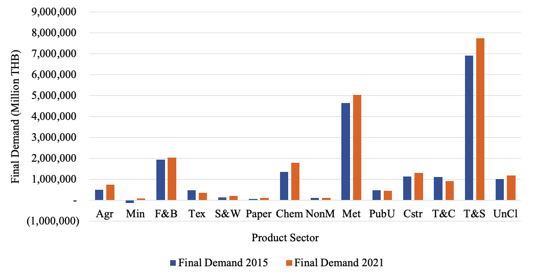
Sectors with already high shares of final demand, especially T&S, continued to dominate and further expand their contribution, indicating a transition toward a more service-oriented economic structure consistent with development trends in emerging economies. In addition, upstream industrial sectors such as metals and chemical products experienced notable increases in final demand, suggesting strong growth in manufacturing and infrastructure-related activities. Resource-based sectors, including Agriculture (Agr) and Mining (Min), also showed positive changes, indicating a recovery in primary production and increased demand for raw materials within the domestic economy.
The SDA assigns a positive final-demand effect of +3.375 Mt CO₂e to the change in total GHG emissions between 2015 and 2021 (Table 4). This component captures the effect of changes in the scale and composition of final demand after holding the production structure and emission coefficients at the polar-decomposition reference conditions. The positive sign indicates that changes in the scale and composition of final demand increased total GHG emissions. Within the IO framework, changes in final demand affect production requirements across the supply chain and can therefore influence both direct and indirect emissions through intersectoral linkages [7]. However, the final-demand effect represents one component of the total change and should be interpreted together with the production-structure and emission-coefficient effects quantified by the SDA.
Table 4. Additive structural decomposition analysis (SDA) of the change in total greenhouse gas (GHG) emissions between 2015 and 2021
|
SDA Component |
Contribution (Mt CO₂e) |
Interpretation |
|
Emission-coefficient effect ($\Delta C^e$) |
+14.468 |
Higher/lower emission coefficients across sectors |
|
Leontief-inverse / production-structure effect ($\Delta C^l$) |
−14.405 |
Change in total production requirements per unit of final demand |
|
Final-demand effect ($\Delta C^y$) |
+3.375 |
Change in the scale and composition of final demand |
|
Net change ($\Delta C$) |
+3.438 |
Sum of the three decomposition components |
Note: Contributions are for the economy-wide total GHG emissions and reconcile to the observed change of 3.438 Mt CO₂e; 2021 monetary data are expressed at constant 2015 prices.
Figure 2 shows that final demand increased in several sectors between 2015 and 2021. Within the SDA, these demand changes contributed +3.375 Mt CO₂e to the economy-wide emission change. This result should be distinguished from the paper-specific final-demand change reported below: the SDA result is an economy-wide decomposition component, whereas the paper-sector comparison describes the monetary change in the paper-products final-demand vector. The corresponding paper-specific embodied emissions are obtained separately by applying the IO model to the paper-specific final-demand vector, yPap, as defined in Section 2.7.
For paper products, final demand increased from 66,515.9 million THB in 2015 to 108,136.2 million THB in 2021 at constant 2015 prices, representing an increase of approximately 62.6%. In current-price terms, the corresponding increase was approximately 69.6%. The difference of about 7.0 percentage points demonstrates that part of the nominal increase reflected sectoral price movements rather than an equivalent increase in real final demand. Accordingly, the constant-price change is used in the temporal comparison and SDA to avoid attributing price changes to changes in real demand.
The distinction between current-price and constant-price final demand is therefore essential for interpreting the temporal change. The price-harmonized framework isolates changes in monetary demand at a common price basis, while the SDA subsequently attributes the economy-wide emission change to final demand, production structure, and emission coefficients.
Furthermore, the expansion of the paper sector (Pap) is closely linked to downstream demand from logistics, trade, and food-related industries. The rapid growth of e-commerce and delivery services has significantly increased the demand for packaging materials, particularly corrugated paper products, reinforcing the role of the Pap as a demand-responsive production sector [29].
3.1.4 Leontief effect (L)
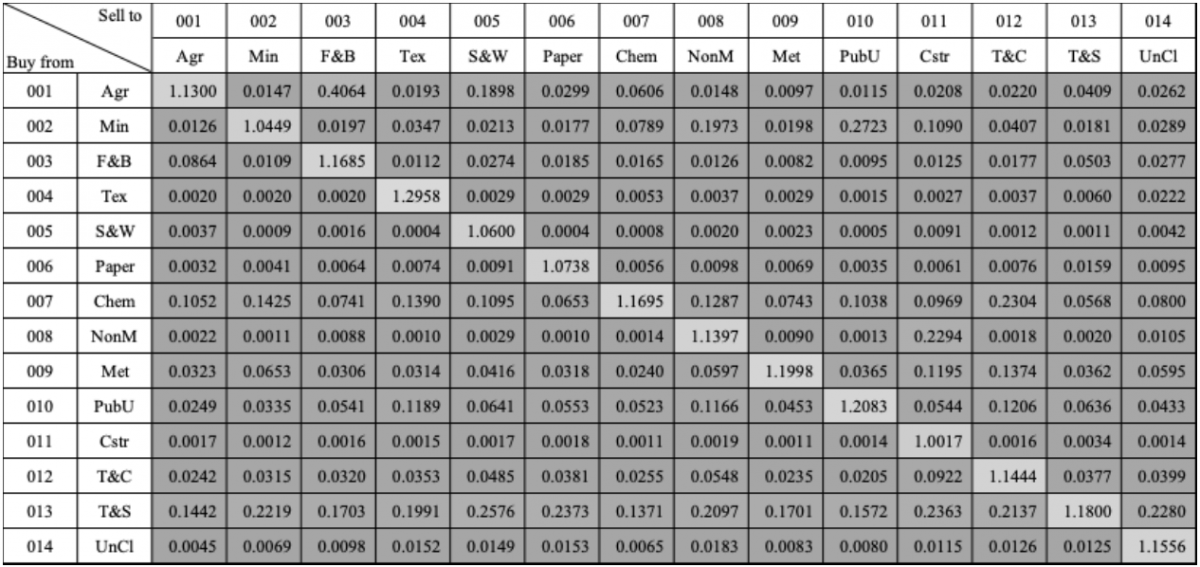
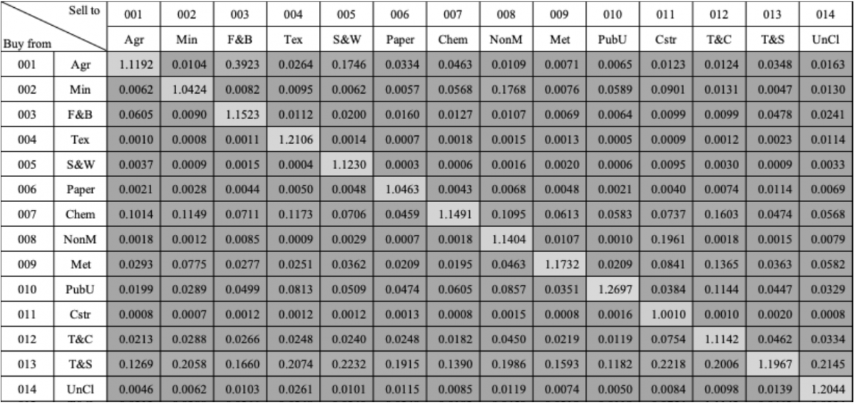
The changes in the Leontief inverse indicate a change in total direct and indirect production requirements associated with final demand. This trend is further illustrated in Figures 3 and 4, which present the Leontief inverse coefficients for 2015 and 2021, respectively. The SDA assigns a negative Leontief-inverse (production-structure) effect of −14.405 Mt CO₂e to the change in total GHG emissions between 2015 and 2021 (Table 4). This negative contribution indicates that changes in the production structure reduced the overall increase in GHG emissions, thereby acting as a major offsetting factor in the total change.
Figure 3. Leontief coefficients, Thailand, 2015
Figure 4. Leontief coefficients, Thailand, 2021
The Leontief inverse represents the total direct and indirect output required from supplying sectors to satisfy one unit of final demand in a receiving sector. For example, the diagonal element for the paper sector (Pap) in Figure 3 is 1.0738, indicating that one THB of paper-sector final demand requires 1.0738 THB of total paper-sector output within the modeled intersectoral structure. Off-diagonal elements represent upstream intersectoral requirements, including inputs from chemical (Chem) and other supplying sectors.
This structural change should be interpreted together with the formal SDA result rather than as a direct measure of process efficiency. For paper products, the diagonal Leontief coefficient decreased from 1.0738 in 2015 to 1.0463 in 2021. For 2021, the Leontief inverse was recalculated from the price-harmonized technical coefficient matrix. The decrease indicates a lower total output requirement associated with one unit of paper-sector final demand within the modeled intersectoral structure. However, a lower Leontief coefficient should not by itself be interpreted as a direct measure of process efficiency; it primarily indicates a change in modeled intersectoral production requirements.
Overall, the negative Leontief-inverse (production-structure) effect substantially offset the positive effects of emission coefficients and final demand. With a contribution of −14.405 Mt CO₂e, this effect represents a major offsetting component of the observed net increase in total GHG emissions between 2015 and 2021.
3.1.5 Emission-coefficient effect (e)
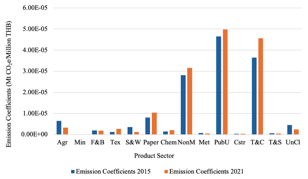
Figure 5 shows the sectoral emission coefficients for 2015 and 2021, while the SDA results in Table 4 indicate that changes in these coefficients contributed +14.468 Mt CO₂e to the change in total GHG emissions between the two years. This component captures changes in sectoral fossil-fuel emission coefficients after accounting for the common-price treatment of monetary output. A positive value indicates that changes in emissions per unit of economic output increased the emissions associated with the modeled production and demand structure.
For paper products, the emission coefficient increased from 8.03 × 10⁻⁶ Mt CO₂e/Million THB in 2015 to approximately 1.04 × 10⁻⁵ Mt CO₂e/Million THB in 2021, representing an increase of approximately 30.0%. This indicates a higher fossil-fuel emission intensity per unit of economic output for paper products on a constant-price basis.
Unlike the negative Leontief-inverse / production-structure effect, the positive emission-coefficient effect exerts upward pressure on total emissions. The SDA result shows that this effect was large enough to offset most of the reduction associated with changes in the production structure.
The simultaneous positive contributions from final demand and emission coefficients indicate that demand expansion alone does not explain the net change. The large negative production-structure contribution demonstrates that changes in intersectoral requirements substantially mitigated the increase. This decomposition provides a more complete basis for identifying mitigation priorities than interpreting any single factor in isolation.
3.1.6 Integrated interpretation of emission drivers
Synthesizing the results, the change in GHG emissions between 2015 and 2021 resulted from substantial and offsetting contributions from changes in final demand, production structure, and emission coefficients. The SDA estimated a positive emission-coefficient effect of +14.468 Mt CO₂e and a positive final-demand effect of +3.375 Mt CO₂e, which were largely offset by a negative Leontief-inverse/ production-structure effect of −14.405 Mt CO₂e. These contributions reconcile to the observed net increase of 3.438 Mt CO₂e. Therefore, the results do not support attributing the net economy-wide emission increase to final demand alone or identifying final demand as the dominant driver.
For paper products, emissions increased from 0.88 Mt CO₂e in 2015 to 1.61 Mt CO₂e in 2021, while constant-price final demand increased by 62.6% and the emission coefficient increased by approximately 30.0%. These changes are consistent with stronger demand and higher fossil-fuel emission intensity in the paper sector. However, the SDA values reported in Table 4 are economy-wide contributions; they should not be interpreted as a paper-sector-specific decomposition of the 0.73 Mt CO₂e increase in paper-product emissions.
The direct-indirect decomposition further demonstrates that a material share of the emissions associated with paper products originates from upstream production requirements outside the Paper sector, particularly PubU and T&S.
The results demonstrate that a relatively modest net change in aggregate emissions can conceal substantially larger offsetting structural effects. Accordingly, mitigation priorities should consider changes in final demand, intersectoral production requirements, and fossil-fuel emission coefficients jointly rather than attributing the observed emission change to a single driver.
3.2 Emission intensity analysis
3.2.1 Emission intensity estimation
The emission intensity of paper products was estimated as the ratio of total GHG emissions from fossil fuel combustion associated with paper products to the corresponding paper-product production volume. In 2015, total emissions were estimated at 876,862.54 t CO₂e, with a paper-product production volume of 6,051,714.93 t, resulting in an emission intensity of 0.1449 t CO₂e/t. In 2021, emissions increased to 1,610,056.67 t CO₂e, while paper-product production was 5,981,693.97 t, resulting in an emission intensity of 0.2692 t CO₂e/t.
Due to the unavailability of a directly observed 2015 production value consistent with the paper-product production definition used in this study, the 2015 paper-product production volume was estimated from observed production data for 2021–2025 obtained from the Industrial Statistics (e-Statistic) of the Office of Industrial Economics (OIE), Ministry of Industry. The observed paper-product production volumes were 5,981,693.97, 5,642,060.12, 5,473,923.82, 5,736,025.41, and 5,721,831.32 t for 2021–2025, respectively. A linear least-squares regression was applied to these observations, yielding an estimated 2015 paper-product production volume of 6,051,714.93 t. This estimate was used as the base-case production denominator for the 2015 emission intensity.
3.2.2 Weighted average Carbon Footprint of Products benchmark
For contextual benchmarking, a comparison was conducted with CFP emission factors developed by TGO [14]. These values were aggregated into a weighted average based on the production structure of paper products in 2021, as summarized in Table 5.
The weighted average CFP benchmark was calculated by combining the emission factors (t CO₂e/t) with the corresponding production volumes of each paper-product category, including paperboard, kraft paper, corrugated and boxboard paper, and printing and writing paper. The weighting reflects the relative contribution of each paper-product category to the total paper-product production volume, thereby representing the production structure of paper products in Thailand. Based on this production-weighted approach, the resulting weighted average CFP benchmark was 1.7144 t CO₂e/t.
Table 5. Data for weighted average Carbon Footprint of Products (CFP) benchmark of paper products in Thailand
|
Paper Types |
Paper-Product Production (t) |
Emission Factor (t CO₂e/t) |
|
Paperboard |
448,065.905 |
1.8679 |
|
Kraft paper |
2,598,549.015 |
1.6324 |
|
Corrugated and boxboard paper |
2,053,978.928 |
1.6184 |
|
Printing and writing paper |
881,100.120 |
2.1020 |
|
Total |
5,981,693.968 |
|
|
Weighted average CFP |
|
1.7144 |
3.2.3 Comparative assessment
The comparison indicates a substantial quantitative difference between the IO-based emission intensity and the production-weighted CFP benchmark. The IO-based emission intensities were 0.1449 t CO₂e/t and 0.2692 t CO₂e/t for 2015 and 2021, respectively, while the production-weighted CFP benchmark was 1.7144 t CO₂e/t.
The difference between the IO-based estimates and the CFP benchmark should be interpreted in light of differences in system boundaries, temporal coverage, product composition, allocation procedures, and sectoral aggregation. The IO-based estimates represent GHG emissions from fossil fuel combustion associated with paper products within a top-down, economy-wide IO framework, whereas the TGO CFP values represent product-level emission factors developed under the CFP assessment framework. Therefore, the quantitative difference between the two estimates does not indicate model overestimation or underestimation and should not be interpreted as evidence of model validity or invalidity. The TGO CFP benchmark is therefore used solely as a contextual reference for interpreting the magnitude of the IO-based emission intensity, rather than as a formal validation criterion.
3.2.4 Results interpretation
The IO-based approach represents a top-down framework capable of capturing both direct and indirect emissions across the economic system, making it suitable for economy-wide analysis. In contrast, CFP values are derived from product-level assessments and provide product-specific emission factors. The difference between the two estimates should therefore be interpreted primarily in terms of differences in methodological scope and data characteristics rather than as evidence of agreement or disagreement in model validity.
In particular, the IO-based estimates and the TGO CFP benchmark differ in temporal coverage, product composition, allocation procedures, system boundaries, and sectoral aggregation. These differences limit the direct comparability of the two estimates. The CFP benchmark therefore provides contextual information on the magnitude of the IO-based emission intensity but does not constitute a formal validation criterion.
Accordingly, the comparison demonstrates the complementary nature of the two approaches: the IO framework provides an economy-wide perspective on emissions associated with intersectoral production linkages, whereas the CFP framework provides product-level emission information. The TGO CFP benchmark is therefore used as a contextual reference rather than as a validation target.
3.2.5 Uncertainty and limitations
This study focuses exclusively on GHG emissions from fossil fuel combustion and excludes non-combustion sources, including industrial process emissions, land-use change, and waste management. Fossil-fuel combustion emissions associated with domestic electricity generation and transportation are not excluded when they are represented by the corresponding PubU and T&C sectors in the IO system. However, emissions associated with activities not represented in the domestic IO and energy datasets are outside the system boundary. A further limitation is that the single-region domestic IO framework does not explicitly trace imported intermediate inputs to their countries of origin. Consequently, upstream GHG emissions associated with foreign production embodied in imported inputs are not captured. This limitation should be considered when interpreting the results as domestic supply-chain emissions rather than consumption-based or global supply-chain emissions. Additional limitations arise from the use of IO tables for 2015 and 2021 and the estimation of production data for 2015 due to data constraints. Minor inconsistencies in reference years across datasets may introduce uncertainties. Nevertheless, the datasets used are considered reliable and are not expected to significantly affect the overall conclusions.
An additional limitation concerns the price harmonization of aggregated IO sectors. Because directly corresponding TPSO price indices were not available for all aggregated sectors, the analysis used the closest available producer or service price indices. For aggregated sectors comprising multiple price categories, a derived sector-level deflator was constructed from the corresponding available indices. For the Unclassified sector, a neutral deflator was applied because no directly corresponding price index was available. These assumptions may introduce uncertainty into sector-level constant-price estimates and should therefore be considered when interpreting the magnitude of sector-specific changes.
The 2015 production denominator is an extrapolated estimate rather than a directly observed value. Its reliability is therefore lower than that of the observed 2021–2025 production data. The estimate was checked against the observed 2021–2025 production trend and further examined using an alternative compound annual growth rate (CAGR)-based extrapolation. The resulting sensitivity range indicates the extent to which the estimated production denominator may affect the reported 2015 emission intensity. Therefore, the 2015 intensity should be interpreted as an estimated value subject to production-data uncertainty rather than as a directly observed intensity.
This study confirms that the IO framework is a robust and policy-relevant tool for evaluating GHG emission intensity at the national level, particularly for paper products, which are characterized by complex intersectoral linkages and high energy dependence. By integrating national energy statistics with IO tables, the approach captures both direct and indirect emissions associated with domestic intersectoral production requirements, enabling a comprehensive understanding of emission drivers within the domestic production system.
The results indicate that the emission intensity of paper products increased between 2015 and 2021. The temporal comparison was conducted using monetary IO data harmonized to a common 2015 price basis, allowing changes in monetary final demand to be interpreted at constant prices. The SDA demonstrates that the observed economy-wide increase in GHG emissions resulted from substantial and offsetting contributions from final demand, production structure, and emission coefficients. Specifically, the final-demand effect contributed +3.375 Mt CO₂e, the Leontief-inverse / production-structure effect contributed −14.405 Mt CO₂e, and the emission-coefficient effect contributed +14.468 Mt CO₂e, yielding the observed net increase of 3.438 Mt CO₂e. These results indicate that the net emission increase cannot be attributed to final demand alone and that mitigation strategies should address demand-side changes, intersectoral production requirements, and fossil-fuel emission coefficients jointly.
The IO-based emission intensities differ from the weighted CFP benchmark, reflecting differences in system boundaries, temporal coverage, product composition, allocation procedures, and sectoral aggregation. Therefore, the CFP comparison is presented solely as a contextual benchmark rather than as a formal validation of the IO-based estimates. The two approaches are complementary: the IO framework provides an economy-wide perspective on direct and indirect emissions associated with intersectoral production linkages, whereas the CFP framework provides product-level emission information.
However, several limitations should be noted, including the exclusion of non-fossil emission sources, the use of sector-matched price deflators where directly corresponding TPSO indices were unavailable, the estimation of production data for 2015 due to data constraints, and the use of a domestic single-region IO framework. Consequently, foreign upstream GHG emissions embodied in imported intermediate inputs are not explicitly captured. The results should therefore be interpreted as emissions associated with domestic production requirements in Thailand rather than as a complete global supply-chain or consumption-based carbon footprint. These limitations may introduce uncertainty into the estimates and should be considered when interpreting the results. Future research should focus on improving data harmonization, incorporating more recent datasets, and developing multi-region or hybrid input–output and Life Cycle Assessment (IO-LCA) approaches to enhance coverage and resolution. Overall, the IO framework provides a complementary economy-wide perspective on the structural determinants of GHG emissions associated with paper products and supports evidence-based policy development for sustainable industrial transformation in Thailand.
|
Aij |
Technical coefficient matrix (dimensionless) |
|
Zij |
Intersectoral transaction matrix (THB) |
|
xj |
Total output vector (THB) |
|
y |
Final demand vector (THB) |
|
I |
Identity matrix (dimensionless) |
|
L |
Leontief inverse matrix $(I-A)^{-1}$ (dimensionless) |
|
Ei |
Direct GHG emissions of sector i (kg CO₂e) |
|
Fi,f |
Fuel consumption of sector i for fuel type f (TJ or ktoe) |
|
EFf |
Emission factor for fuel type f (kg CO₂e unit fuel-1) |
|
ei |
Emission coefficient of sector i (kg CO₂eTHB-1) |
|
C |
Total GHG emissions (kg CO₂e) |
|
EIpaper |
Emission intensity of paper products (t CO₂et-1) |
|
Cpaper |
Total emissions of paper products (t CO₂e) |
|
Qpaper |
Production volume of paper products (t) |
|
f |
Fuel type index (dimensionless) |
|
i, j |
Sector indices (dimensionless) |
|
yj |
Sector-specific final-demand vector (THB) |
|
yPap |
Paper-specific final-demand vector (THB) |
|
Ci |
GHG emissions embodied in the final demand of sector j (kg CO₂e) |
|
CPap |
Total emissions embodied in paper-sector final demand (kg CO₂e) |
[1] IPCC. (2022). Climate Change 2021: The Physical Science Basis. Cambridge University Press. https://doi.org/10.1017/9781009157896
[2] UNECE & FAO. (2023). Data brief: Pulp, paper and paperboard. https://unece.org/sites/default/files/2023-11/2023-data-brief-pap-final-web_1.pdf.
[3] OIE. (2021). Sectoral industrial economic conditions of Thailand in 2021 and outlook for 2022. https://www.oie.go.th/assets/portals/1/files/monthly_report/anualreport2021_for2022.pdf.
[4] DEDE. (2021). Thailand energy balance 2021. https://www.dede.go.th/uploads/Thailand_Energy_Commodity_Account_2021_edit_181067_95b4724f1f.xlsx?updated_at=2024-10-18T02:26:17.113Z.
[5] Dias, A.C., Arroja, L., Capela, I. (2007). Carbon dioxide emissions from forest operations in Portuguese eucalypt and maritime pine stands. Scandinavian Journal of Forest Research, 22(5): 422-432. https://doi.org/10.1080/02827580701582692
[6] Leontief, W.W. (1936). Quantitative input and output relations in the economic system of the United States. The Review of Economics and Statistics, 18(3): 105-125. https://doi.org/10.2307/1927837
[7] Miller, R.E., Blair, P.D. (2009). Input–Output Analysis: Foundations and Extensions. Cambridge University Press. https://doi.org/10.1017/CBO9780511626982
[8] Tukker, A., Dietzenbacher, E. (2013). Global multiregional input–output frameworks: An introduction and outlook. Economic Systems Research, 25(1): 1-19. https://doi.org/10.1080/09535314.2012.761179
[9] Wiedmann, T. (2009). A review of recent multi-region input–output models. Ecological Economics, 69(2): 211-222. https://doi.org/10.1016/j.ecolecon.2009.08.026
[10] Lenzen, M. (2001). Errors in conventional and input–output-based life-cycle inventories. Journal of Industrial Ecology, 4(4): 127-148. https://doi.org/10.1162/10881980052541981
[11] Su, B., Ang, B.W. (2012). Structural decomposition analysis applied to energy and emissions: Some methodological developments. Energy Economics, 34(1): 177-188. https://doi.org/10.1016/j.eneco.2011.10.009
[12] DEDE. Thailand energy statistics: 2015 and 2021 reports. https://www.dede.go.th/articles?id=467&menu_id=49, accessed on Jul. 8, 2026.
[13] DEDE. (2015). Thailand energy balance 2015. https://www.dede.go.th/uploads/2558_Table_of_Thailand_Energy_Balance_2015_4fd82edc90.xlsx?updated_at=2023-02-26T16:30:48.871Z.
[14] TGO. (2022). Carbon footprint of product: Emission factor (CFP). http://thaicarbonlabel.tgo.or.th/.
[15] NESDC. Input–output tables of Thailand (2015 & 2021). https://www.nesdc.go.th/en/info/input-output-tables-i-o-tables-en/, accessed on Feb. 5, 2026.
[16] IPCC. (2006). 2006 IPCC Guidelines for National Greenhouse Gas Inventories. https://www.ipcc-nggip.iges.or.jp/public/2006gl/.
[17] IPCC. (2019). 2019 Refinement to the 2006 IPCC Guidelines for National Greenhouse Gas Inventories. https://www.ipcc-nggip.iges.or.jp/public/2019rf/.
[18] Peters, G.P., Hertwich, E.G. (2008). CO₂ embodied in international trade with implications for global climate policy. Environmental Science & Technology, 42(5): 1401-1407. https://doi.org/10.1021/es072023k
[19] CEIC Data. (2026). Thailand producer price index: 2015=100: Classification of production by activities (CPA): Weights. https://www.ceicdata.com/en/thailand/producer-price-index-2015100-classification-of-production-by-activities-cpa-weights.
[20] Dietzenbacher, E., Hoen, A.R. (1998). Deflation of input–output tables from the user's point of view: A heuristic approach. Review of Income and Wealth, 44(1): 111-122. https://doi.org/10.1111/j.1475-4991.1998.tb00255.x
[21] Dietzenbacher, E., Temurshoev, U. (2012). Input–output impact analysis in current or constant prices: Does it matter? Journal of Economic Structures, 1: 4. https://doi.org/10.1186/2193-2409-1-4
[22] Minx, J., Wiedmann, T., Wood, R., et al. (2009). Input–output analysis and carbon footprinting: An overview of applications. Economic Systems Research, 21(3): 187-216. https://doi.org/10.1080/09535310903541298
[23] Leontief, W.W. (1951). Input–output economics. Scientific American, 185(4): 15-21. https://doi.org/10.1038/scientificamerican1051-15
[24] Ang, B.W. (2004). Decomposition analysis for policymaking in energy: Which is the preferred method? Energy Policy, 32(9): 1131-1139. https://doi.org/10.1016/S0301-4215(03)00076-4
[25] IEA. (2020). Energy Efficiency 2020. https://www.iea.org/reports/energy-efficiency-2020.
[26] Hoekstra, R., van den Bergh, J.C.J.M. (2003). Comparing structural decomposition analysis and index. Energy Economics, 25(1): 39-64. https://doi.org/10.1016/S0140-9883(02)00059-2
[27] Dietzenbacher, E., Los, B. (1998). Structural decomposition techniques: Sense and sensitivity. Economic Systems Research, 10(4): 307-324. https://doi.org/10.1080/09535319800000023
[28] Lenzen, M., Wood, R., Wiedmann, T. (2010). Uncertainty analysis for multi-region input–output models: A case study of the UK's carbon footprint. Economic Systems Research, 22(1): 43-63. https://doi.org/10.1080/09535311003661226
[29] OECD. (2020). E-Commerce in the Time of COVID-19. https://doi.org/10.1787/3a2b78e8-en