
Nur Vadila Putri* | Anas Iswanto Anwar | Hamrullah
© 2026 The authors. This article is published by IIETA and is licensed under the CC BY 4.0 license (http://creativecommons.org/licenses/by/4.0/).
OPEN ACCESS
Narrowing regional disparities in human development is a policy priority under Indonesia’s fiscal decentralisation, yet whether gains in one province spread to its neighbours or merely track a shared national trend remains unclear. Using a balanced panel of Indonesia’s 33 provinces (2010–2024, 495 observations), we relate the Human Development Index (HDI) to income inequality and government expenditure through a spatial Durbin model (SDM) that nets out the shared national trajectory. Once this trend is removed, the direct spillover through HDI itself is small (ρ = −0.08) and statistically indistinguishable from zero under both asymptotic and block-bootstrap inference, evidence against a direct diffusion channel. Economic activity is more robust: a province’s own gross regional domestic product carries a positive indirect association with neighbours’ HDI, significant across alternative neighbour definitions, though its magnitude (1.2–7.7) is sensitive to those choices. Own-province health expenditure is negatively associated with own-province HDI, consistent with compensatory allocation toward lagging provinces rather than a harmful effect of spending. Policymakers should not assume that human-development gains diffuse automatically to neighbouring provinces; regional economic integration, not proximity to high-HDI neighbours, is the more credible channel for cross-provincial gains under decentralisation.
fiscal decentralisation, Human Development Index, Indonesia, regional disparity, spatial spillover, sustainable development
Averaged across Indonesia’s provinces, the Human Development Index (HDI) rose from 65.6 in 2010 to 73.6 in 2024, yet provincial disparities remain stark: Papua’s average over that period, 60.8, sits nearly nine points below the 33-province mean, while Jakarta and Yogyakarta have both passed 80 in recent years. Closing this within-country gap is a recurring commitment of Indonesia’s fiscal decentralisation policy and is central to its sustainable development agenda, which links human development to health, education, and reduced inequality [1]. Two very different stories could explain the narrowing: progress in one province might genuinely spread to its neighbours through rising income or public investment, or every province might simply be riding the same national wave. Distinguishing between them bears directly on how decentralisation and place-based development policy should be evaluated.
A substantial literature has examined the correlates of provincial and district-level human development in Indonesia, typically treating each region as independent of its neighbours [2-5]. A related strand studies how fiscal decentralisation shapes regional convergence using spatial methods, but at the district level and with a focus on economic growth rather than HDI directly [6, 7]. A smaller body looks explicitly at spatial dependence in HDI, though only at the single-province level and only as conference proceedings, both focused on Central Java rather than the full national panel [8, 9]. One question remains largely unexamined: whether human development itself genuinely spreads across provincial borders at the national level, once the shared national trend, which moves every province in the same direction and mechanically makes them look alike, is separated from spillovers proper.
This paper studies regional disparities and spillovers in human development for a balanced panel of all 33 Indonesian provinces from 2010 to 2024. We define each province’s neighbours by its three geographically nearest provincial centroids rather than shared land borders, a choice that suits Indonesia’s archipelagic geography, where six of the 33 provinces have no land neighbour at all. We also allow for unobserved, lasting differences between provinces. To separate the shared national trend from genuine cross-province relationships, we compare each province, in each year, to that year’s national average, letting us ask whether provinces are converging toward one another or merely moving in parallel.
Once the national trend is removed, the estimated spillover through HDI itself is small, negatively signed, and statistically indistinguishable from zero under both asymptotic and block-bootstrap inference, evidence against a direct HDI-to-HDI diffusion channel. What spreads more reliably is economic activity: a rise in a province’s own economic output is associated with a positive spillover to neighbouring provinces’ HDI that survives bootstrap resampling and remains significant, though unstable in magnitude, across alternative neighbour definitions. Own-province health expenditure tells a different story, carrying a robust negative association with own-province HDI. This is more consistent with compensatory allocation of health funds toward lagging provinces than with an adverse effect of spending: provinces with lower human development appear to receive larger remedial transfers.
We take particular care to distinguish genuine regional relationships from artefacts of the shared national trend. Before settling on our preferred approach, we estimated the same relationships without any trend adjustment and with calendar-year controls. The apparent spillover through HDI collapsed from strongly significant, when left uncorrected, to indistinguishable from zero under either trend-control strategy, a pattern unlikely to arise from noise. Two further checks support this reading: an independent reproduction using an unrelated statistical package matches our primary results closely, and a cross-check against an alternative estimator finds full agreement in the direction of all twelve shared relationships. We also subject every result to a resampling-based robustness check, flagging as fragile any finding that loses significance; the direct relationship between a province’s own economic output and its own HDI is one such case, which we do not treat as robust.
This paper contributes to sustainable regional development in Indonesia in three ways. First, we add an explicitly geographic dimension to the literature on determinants of Indonesian human development [2-5], which has generally treated provinces as independent, clarifying whether a province’s development is shaped only by its own conditions or also by its neighbours’. Second, we extend the spatial approach to the full 33-province national panel, with an explicit decomposition of direct and indirect effects on HDI, so that policymakers can distinguish which provinces benefit mainly from their own investments and which stand to gain from their neighbours’ growth, a distinction that matters for how decentralised spending is targeted; this builds on both the single-province HDI studies [8, 9] and the district-level convergence studies focused on economic growth [6, 7]. Third, and most consequential for policy, we show that Indonesia’s apparent convergence in human development across neighbouring provinces reflects a shared national trajectory rather than genuine cross-provincial diffusion: place-based policies presuming that HDI gains spread automatically to neighbours are not supported by the evidence, whereas regional economic integration offers a more credible channel through which one province’s progress can benefit its neighbours.
A first strand examines the determinants of provincial human development in Indonesia using standard, non-spatial panel methods. Whether government spending translates into development gains is itself a live question: an assessment using authorised data over 2015–2021 finds only a modest positive effect and stresses that the quality of spending, not its volume, determines whether budget realisation yields genuine gains [10]. District-level evidence finds that own-source income and special allocation funds raise HDI and its components, while general allocation and revenue-sharing funds are negatively associated with it, read as favouring fiscal independence over central transfers [2]. Regional GRDP, village-fund allocations, and poverty jointly shape HDI across the 33 provinces over 2015–2022 [3], and a subnational human capital index shows that within-province variation can be masked by a single province-level figure [11]. Using Arellano–Bond dynamic panel generalized method of moments (GMM) across 34 provinces (2011–2020), fiscal decentralisation, financial dependence, and education and economic-affairs spending accelerate convergence while health spending slows it [4], echoing the negative health-expenditure association we report below. Fiscal independence likewise conditions the joint relationship between decentralisation, human development, and growth across districts [5], consistent with evidence that decentralisation funds, growth, and public expenditure jointly drive development outcomes across autonomous regions [12]. Decentralisation also carries a distributional cost: decentralising revenue authority is associated with higher regional income inequality, so the same lever we study can widen the disparities HDI is meant to summarise [13]. These levers depend on adequate governance capacity [14, 15] and operate in a country that must raise its aggregate growth path by narrowing regional disparities in productive capacity [16]. No study in this strand models cross-regional spatial dependence explicitly.
A second, smaller strand applies spatial econometric methods to HDI itself, almost exclusively at the single-province level and via conference proceedings: a spatial Durbin error model finds spatial error (SEM) dependence in the life-expectancy, schooling, and purchasing-power components of HDI across the districts of Central Java [8], and an alternative spatial panel specification for the same province reaches a similar conclusion [9]. A rigorously reviewed treatment of spatial dependence in HDI, even at this scale, therefore remains largely absent. Closely related work on district-level growth and convergence does find significant spatial spillovers from fiscal decentralisation [6], and across 514 districts (2010–2018), a district’s HDI and GDP per capita both grow faster when its neighbours’ values are high [7].
Spatial dependence in regional welfare more broadly has been documented for eastern Indonesia, the same region our Getis–Ord analysis identifies as an economic cold spot [17], and for poverty across the Pantura districts of East Java [18]; it extends even to disaster economics, where the growth effect of natural-disaster damage depends on a district’s own HDI and spills over to its neighbours [19]. Comparable geographic dependence is well documented outside Indonesia, indicating a general feature of regional development data rather than an Indonesian artefact: spatial inequality tied to infrastructure access in Karnataka, India [20]; provincial clustering in China’s HDI attributed to shared growth corridors [21]; spatial heterogeneity in a carbon-emission-sensitive HDI in China’s Poyang Lake Basin [22]; and improved forecast accuracy from incorporating neighbouring-region information in Morocco [23]. This literature establishes that spatial methods are informative for regional human-development data generally, and for Indonesian data at the district level; it has not, to our knowledge, been applied to HDI on the full 33-province national panel over fifteen years, a setting in which separating genuine spillovers from a shared national time trend becomes empirically first-order.
A third strand examines the channels through which public expenditure shapes the HDI components that this paper’s covariates capture. Life expectancy across Indonesian provinces responds to health-infrastructure provision alongside political and socioeconomic status [24], showing that HDI’s longevity dimension is sensitive to health-sector allocation. Education quality is linked directly to HDI outcomes, reinforcing why government education expenditure is a natural covariate rather than an incidental control [25]. The institutional channel matters too: governance quality and fiscal decentralisation exhibit bidirectional causality in Indonesia, whereas no such relationship holds for growth, implying that institutional quality mediates decentralisation’s effect on development [26]. Income and poverty converge only partially across Indonesian local governments under decentralisation, more so for income than poverty [27], consistent with our finding that convergence in one development outcome need not imply convergence in another.
A fourth consideration, cutting across all three strands, concerns what a coefficient in this kind of model reveals about a province’s human development. When provinces are geographically linked, a change in one can echo through to its neighbours before settling into a new pattern, so a raw coefficient understates or overstates a variable’s full contribution depending on how far that echo travels [28]. Separating this into direct and indirect effects is accordingly standard in applied spatial work; among the studies reviewed, only one reports such a decomposition [7], and only for HDI as a convergence outcome rather than for the covariates, expenditure, inequality, and economic scale that determine its level. We adopt the decomposition throughout for these covariates directly, so as not to conflate who benefits: the province itself or its neighbours.
3.1 Data
Our data form a balanced panel of Indonesia’s 33 provinces observed annually from 2010 to 2024 (T = 15), yielding 495 province-year observations. The dependent variable is the provincial HDI, known domestically as the Indeks Pembangunan Manusia, a composite indicator of longevity, education, and standard of living compiled by Indonesia’s national statistics agency (BPS) following United Nations Development Programme (UNDP) methodology. Explanatory variables are the provincial Gini ratio, a measure of income inequality, and the natural logarithms of provincial government expenditure in four functional categories: economic affairs, health, education, and social protection, labelled in the tables ln(Economic affairs), ln(Health), ln(Education), and ln(Social protection). We additionally control for the natural log of provincial gross regional domestic product, ln(GRDP), the principal measure of a province’s overall resource base, plausibly correlated with both expenditure levels and human development outcomes.
Indonesia’s official province count rose from 33 to 38 during our sample period, with North Kalimantan splitting from East Kalimantan in 2012 and four new Papua provinces (South Papua, Central Papua, Highland Papua, and Southwest Papua) created in 2022–2023. Our panel nonetheless holds a fixed 33-province geography throughout 2010–2024 because the underlying BPS-derived series reports HDI and expenditure at the original 33-province level for its entire published history, folding the newer provinces’ figures back into their pre-split parents rather than reporting them separately. We inherit this boundary convention from the source series rather than re-aggregating independently, and match our spatial weight matrix to the same 33-province geography (Section 3.2). Expenditure variables are nominal rather than inflation- or population-adjusted; Section 5 discusses the implications.
No observations are lost to missing data: all 495 province-year cells have non-missing values on every variable, so the analytic sample equals the raw sample. All 33 provinces were also successfully matched to their corresponding administrative boundaries in the shapefile used to construct the spatial weight matrix (Section 3.2).
Table 1. Descriptive statistics
|
Variable |
Mean |
SD |
Min |
Max |
|
HDI |
69.607 |
4.659 |
54.450 |
83.080 |
|
Gini ratio |
0.361 |
0.041 |
0.236 |
0.459 |
|
ln(Economic affairs) |
26.985 |
0.888 |
24.293 |
30.313 |
|
ln(Health) |
26.744 |
1.048 |
23.837 |
30.022 |
|
ln(Education) |
27.615 |
1.345 |
22.086 |
30.712 |
|
ln(Social protection) |
24.869 |
0.905 |
21.825 |
28.991 |
|
ln(GRDP) |
11.878 |
1.170 |
9.615 |
14.582 |
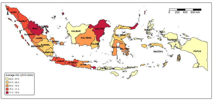
Table 1 shows substantial cross-provincial dispersion in HDI (range 54.5–83.1) alongside a comparatively narrow range in the Gini ratio (0.24–0.46), consistent with Indonesia’s pattern of large level differences in development outcomes across regions coexisting with more modest differences in within-province inequality. Figure 1 maps this dispersion, averaged over 2010–2024. The highest averages are Jakarta (79.7), Yogyakarta (78.6), East Kalimantan, Kepulauan Riau, Bali, Riau, and North Sulawesi; the lowest are Papua (60.8), West Papua, East Nusa Tenggara, West Sulawesi, West Kalimantan, West Nusa Tenggara, North Maluku, and Gorontalo.
Figure 1. Average Human Development Index (HDI) by province, 2010–2024
3.2 Spatial weight matrix
We construct the spatial weight matrix W from provincial centroids using k-nearest-neighbour (KNN) relations with k = 3, row-standardised. We prefer KNN to contiguity-based weights because Indonesia’s archipelagic geography leaves many provinces without a shared land border: under queen contiguity, six of the 33 provinces have no contiguous neighbour and the structure decomposes into eleven disconnected sub-graphs, an expected outcome where administrative adjacency does not track physical adjacency, rendering contiguity unsuitable as the primary weight matrix. We use KNN matrices with k = 5 and k = 8 for sensitivity analysis (Section 4.5). Scale matters: spatial decomposition of provincial sustainability indicators is highly sensitive to the administrative scale at which the underlying indicator is aggregated, a scale-mismatch problem documented most recently for Vietnam’s provincial indicator system [29].
3.3 Model specification
Answering whether a province’s human development is shaped by its neighbours, and not only its own circumstances, requires a model that lets both channels operate at once: a province’s HDI may respond directly to a neighbour’s HDI, and separately to a neighbour’s income, inequality, or public spending. We estimate a spatial Durbin model (SDM), which nests both the spatial autoregressive (SAR) and SEM specifications as special cases and allows spillovers through both the outcome and the explanatory variables [30, 31], consistent with broader developments in spatial panel data modelling [32]:
$\begin{aligned} & \mathrm{HDI}_{i t}=\alpha+\rho \sum_j W_{i j} \mathrm{HDI}_{j t}+\beta^{\prime X_{i t}} \, +\theta^{\prime} \sum_j W_{i j} X_{j t}+\mu_i+\varepsilon_{i t}\end{aligned}$ (1)
where, i indexes provinces (i = 1, …, 33), t indexes years (t = 2010, …, 2024), Xit is the vector of six covariates described in Section 3.1, W is the row-standardised KNN spatial weight matrix, ρ is the SAR coefficient, θ is the vector of spatial-lag (WX) coefficients, and μi is a province-specific random effect. The parameter ρ captures dependence through the outcome: a shock to HDI in one province propagates mechanically to its neighbours under the model's structure, while θ captures dependence through observable covariates. We do not interpret β and θ as marginal effects directly; instead, we report the decomposed direct, indirect, and total effects implied by the spatial multiplier (I − ρW)−1, obtained via parametric Monte Carlo simulation (R = 1,000 draws) from the asymptotic covariance matrix of the estimated parameters [28]. The SDM is not specific to human-development applications: the general case for this specification, and for basing inference on indirect effects rather than raw coefficients, is well established in the wider applied spatial econometrics literature [33], and the specification suits any setting in which an outcome may respond to both a region's own covariates and its neighbours'.
3.4 Time-effect control
A two-way random-effects specification, absorbing both province- and year-specific heterogeneity, is the natural benchmark for a panel of this structure, but the maximum-likelihood spatial estimator we use (splm::spml in R) does not support two-way random effects for spatial models [34]. We therefore control for common national trends through cross-sectional yearly demeaning: before estimation, we subtract from HDI, from each covariate, and from each covariate’s spatial lag the cross-sectional (33-province) mean of that variable in the same year. For a row-standardised weight matrix, this operation commutes with spatial lagging, so demeaning before or after constructing WX yields identical results. It is algebraically equivalent to sweeping out a deterministic time fixed effect, a standard device when software does not support a formal two-way specification [35]. Separating a genuine common factor, such as a shared national trend, from cross-sectional dependence that reflects real unit-to-unit relationships is a recognised identification problem; conflating the two generates spurious evidence of dependence [36]. A fully interactive fixed-effects estimator would model such a factor directly rather than remove it by demeaning [37], but none is currently available for the specification required here. We therefore treat cross-sectional demeaning as an approximation rather than a formally equivalent two-way estimator, and return to this limitation in Section 5.
Cross-sectional demeaning carries an econometric cost worth making explicit. Because each year’s 33 province-level deviations from the cross-sectional mean sum to zero by construction, the demeaned variables cannot be independent across provinces even when the underlying data are: for N units demeaned each year, the expected pairwise correlation among purely idiosyncratic, mean-zero disturbances is mechanically −1/(N − 1), about −0.03 for our 33 provinces. This mechanical negative dependence is a standard consequence of within-year demeaning, not a peculiarity of our design, but has not previously been discussed in this literature: it could in principle bias the SAR coefficient ρ and the SEM coefficient λ, both estimated as negative, toward negative values. We doubt it is the primary explanation. At roughly −0.03, it is well under half the magnitude of the SDM (RE) estimate of ρ (−0.079) and about a tenth of the spatial Durbin error model (SDEM) (FE) estimate of λ (−0.320), so it cannot account for either coefficient’s full size even if it contributes to the sign. We nonetheless flag this as an open limitation rather than treat the negative sign of ρ and λ as fully settled; Section 5 returns to it.
3.5 Model selection and estimator choice
We select among SAR, SEM, and SDM specifications using robust Lagrange multiplier (LM) tests for spatial lag and SEM dependence [38]. We further test the common-factor restriction implied by the SEM specification, θ = −ρβ, via a likelihood-ratio test comparing the SDM and SEM log-likelihoods; rejection of this restriction indicates that the SDM cannot be simplified to a SEM [39].
We choose between random- and fixed-effects estimators using the spatial Hausman test, implemented separately for the spatial-lag and spatial-error branches [40]. Once cross-sectional demeaning is applied, the test rejects random effects for both branches, which would ordinarily favour fixed effects. We nonetheless report our preferred SDM under random effects, for a reason specific to the spatial-lag branch rather than a disregard of the Hausman result. Within-transformation maximum-likelihood estimation of a SAR parameter is asymptotically biased of order O(1/T) in panels with a fixed time dimension, an incidental-parameters problem that does not afflict the spatial-error specification, whose fixed-effects estimator remains consistent under the same asymptotics [41]. Because splm implements no bias-corrected estimator, a fixed-effects estimate of the spatial-lag branch would substitute a known small-T bias in ρ for the orthogonality violation the Hausman test detects, rather than resolving it. We therefore retain random effects for the SDM, and report the fixed-effects SDEM as a cross-check on the error branch, where no such asymmetry applies. We do not compare information criteria across the two, whose likelihoods are non-comparable: the fixed-effects estimator profiles out individual effects without counting them as parameters, while the random-effects estimator integrates over them via estimated variance components [42].
Rather than resting this choice on the incidental-parameters argument alone, we also estimate the naive fixed-effects SDM for the spatial-lag branch and compare it with our preferred random-effects specification (Table A1), so readers can judge the difference for themselves [41]. One specification issue deserves note: variance inflation factors on the spatially lagged regressors reach 9.1 for W × ln(Health), 10.5 for W × ln(Social protection), and 11.7 for W × ln(GRDP), so the spatial lags are correlated with one another, as is common when several covariates share the same neighbourhood structure. This inflates standard errors rather than biasing coefficients; we therefore read the individually insignificant spatial lags (W × ln(Health), W × ln(Education), and W × ln(Social protection)) as imprecisely estimated rather than established nulls, while the two we interpret, W × ln(GRDP) and W × ln(Economic affairs), remain significant.
3.6 Inference
Because maximum-likelihood inference in spatial panel models relies on asymptotic normality, a poor approximation with only 33 cross-sectional units, we complement asymptotic standard errors with a non-parametric block-year bootstrap. In each of 2,000 replications, we resample the fifteen years with replacement, rebuild the spatially lagged covariates, and re-estimate the full model; the resulting empirical distribution of each coefficient yields a bootstrap standard error, a continuity-corrected two-sided p-value, and a 95 percent percentile confidence interval, none relying on asymptotic normality. We test residual normality with the Shapiro–Wilk test and, where it is rejected, treat the bootstrap inference as the more reliable basis for judging significance.
We additionally assess robustness to the choice of spatial weight matrix by re-estimating the model with k = 5 and k = 8 nearest neighbours, and to the influence of individual provinces through a leave-one-province-out jackknife, in which the model, including the spatial weight matrix and spatially lagged covariates, is fully reconstructed and re-estimated 33 times, once with each province excluded. Because a jackknife of this kind flags only coefficients that change sign, we additionally re-estimate the full model with the single most influential province excluded and compare coefficients and p-values directly against the full-sample estimates, so that a coefficient that loses statistical support without reversing sign is not overlooked (Section 4.6).
Throughout, we interpret our estimates as associations rather than causal effects. Provincial government expenditure is plausibly endogenous to human development outcomes, both because higher-capacity provincial governments may systematically allocate spending differently and because central government transfers often respond to a province's development status, a form of reverse causality this design cannot rule out. We do not employ an instrumental-variables or GMM strategy for the spatial panel setting, and we discuss this limitation in Section 5.
This section reports our results against the objective set out in Section 1: whether human development in Indonesia’s provinces genuinely spreads to neighbours, or merely appears to converge because every province follows the same national trajectory. Sections 4.1 to 4.5 present the model-selection diagnostics, main estimates, and robustness checks; Section 4.6 adds a province-level robustness check; Section 4.7 tests whether a shared national trend, rather than genuine cross-provincial relationships, explains our results; and Section 4.8 interprets the policy-relevant findings that survive this scrutiny.
4.1 Model selection diagnostics
Both robust LM tests for spatial lag and SEM dependence are statistically significant, supporting the more general spatial Durbin specification over either the SAR or SEM alone (Table 2).
Table 2. Model selection diagnostics
|
Test |
Statistic |
df |
p-Value |
Conclusion |
|
Robust LM – spatial lag |
47.310 |
1 |
<0.001 |
Significant |
|
Robust LM – spatial error |
54.033 |
1 |
<0.001 |
Significant |
|
Spatial Hausman – lag branch |
109.72 |
6 |
<0.001 |
FE required |
|
Spatial Hausman – error branch |
152.62 |
6 |
<0.001 |
FE required |
|
Common-factor test (SDM vs SEM) |
63.283 |
6 |
<0.001 |
SDM required |
Notes: All tests estimated on data controlled for common time trends via cross-sectional yearly demeaning (Section 3.4). “FE required” indicates rejection of the random-effects null at the 5 percent level. Standard (non-robust) LM tests and the classical (non-spatial) Hausman test were also computed and agree in conclusion: spatial Durbin model (SDM), fixed effects (FE).
The common-factor test decisively rejects the restriction implied by the SEM specification (χ2 = 63.28, df = 6, p < 0.001), confirming that the SDM cannot be simplified to a SEM. The spatial Hausman test rejects random effects for both branches of the model once cross-sectional demeaning is applied (p < 0.001 in every case), a marked change from the same test applied to the raw, undemeaned data: there, it failed to reject random effects for the spatial-lag branch (p = 0.109; the classical, non-spatial Hausman test applied to the same raw data agrees, p = 0.275). We discuss this reversal, which we independently verify with an unrelated software implementation, in Section 4.7.
4.2 Main results
Table 3 reports our preferred random-effects SDM alongside the fixed-effects SDEM estimated on the error branch, where fixed effects is unambiguously correct; Section 3.5 gives our reasons for retaining random effects on the lag branch. We treat the SDEM as a cross-check: all twelve coefficients shared between the two specifications agree in sign.
The SAR coefficient ρ is small and negatively signed (−0.079); Section 4.4 shows it is not statistically distinguishable from zero under either asymptotic or bootstrap inference, a null we interpret there and situate within the paper’s broader conclusion in Section 4.7. Own-province ln(GRDP) and ln(Health) both carry large, significant negative coefficients. The spatial lags of ln(GRDP) and ln(Economic affairs) are both significant but of opposite sign: neighbouring GRDP is associated with higher own-province HDI, neighbouring economic-affairs expenditure with lower. Because raw SDM coefficients lack a direct marginal-effect interpretation, we turn to the decomposed effects in Section 4.3 before interpreting magnitudes.
Table 3. Main results and fixed-effects cross-check
|
Variable |
SDM (RE) |
SE |
SDEM (FE) |
SE |
|
Gini ratio |
1.462 |
1.945 |
1.372 |
1.898 |
|
ln(Economic affairs) |
0.232** |
0.111 |
0.307*** |
0.109 |
|
ln(Health) |
−0.424*** |
0.107 |
−0.444*** |
0.105 |
|
ln(Education) |
−0.045 |
0.071 |
−0.037 |
0.068 |
|
ln(Social protection) |
0.041 |
0.083 |
0.041 |
0.079 |
|
ln(GRDP) |
−3.400*** |
0.298 |
−4.208*** |
0.300 |
|
W × Gini ratio |
−7.149** |
3.200 |
−5.232* |
2.812 |
|
W × ln(Economic affairs) |
−0.731*** |
0.190 |
−0.772*** |
0.171 |
|
W × ln(Health) |
0.228 |
0.183 |
0.399** |
0.166 |
|
W × ln(Education) |
0.044 |
0.124 |
0.094 |
0.108 |
|
W × ln(Social protection) |
0.055 |
0.201 |
0.048 |
0.178 |
|
W × ln(GRDP) |
3.809*** |
0.537 |
4.925*** |
0.513 |
|
ρ (spatial AR) / λ (spatial error) |
−0.079 |
0.069 |
−0.320*** |
0.064 |
|
Observations |
495 |
|
495 |
|
Notes: SDM (RE) estimated with model = random, effect = individual, retained under random effects for the reason given in Section 3.5; SDEM (FE) with model = within, effect = individual, spatial.error = “b” [43]. Asymptotic standard errors are reported in the adjacent SE columns. * p < 0.10, ** p < 0.05, *** p < 0.01.
4.3 Direct, indirect, and total effects
We decompose the SDM (RE) estimates into direct, indirect, and total effects by the Monte Carlo procedure set out in Section 3.3 (Table 4) [28].
Table 4. Direct, indirect, and total effects
|
Variable |
Direct |
Indirect |
Total |
|
Gini ratio |
1.546 |
−7.032** |
−5.487 |
|
ln(Economic affairs) |
0.247** |
−0.707*** |
−0.460** |
|
ln(Health) |
−0.432*** |
0.245 |
−0.186 |
|
ln(Education) |
−0.046 |
0.044 |
−0.002 |
|
ln(Social protection) |
0.043 |
0.042 |
0.085 |
|
ln(GRDP) |
−3.474*** |
3.862*** |
0.387 |
Notes: * p < 0.10, ** p < 0.05, *** p < 0.01, based on the empirical distribution of 1,000 Monte Carlo simulations from the estimated asymptotic covariance matrix of the SDM (RE).
The indirect effect of ln(GRDP), 3.862 (p < 0.001), is the largest and most precisely estimated spillover in the model: a province’s neighbours show higher HDI when that province’s GRDP is higher, holding those neighbours’ covariates fixed. Its direct effect, −3.474, is of opposite sign and, as Section 4.4 shows, does not survive bootstrap inference; the total effect, 0.387, is therefore a poor summary of either component and should not be reported without the decomposition. A negative direct association between a province’s own GRDP and its own HDI may seem inconsistent with HDI’s standard-of-living dimension, but that dimension is an income proxy BPS constructs from provincial purchasing-power expenditure rather than from GRDP. The two are conceptually distinct: GRDP measures aggregate production within a province’s borders, including output from non-resident labour and capital and from sectors such as mining whose returns do not translate directly into resident household consumption, whereas HDI’s income component tracks average household purchasing power. A province can thus record rising GRDP without a matching rise in the living-standard component BPS uses, consistent with, though not establishing, the negative direct coefficient. We revisit the GRDP indirect magnitude in Sections 4.5 and 4.6, where it proves sensitive to the weight matrix and to the exclusion of individual provinces, though its sign and significance do not. The indirect effect of the Gini ratio is negative and significant (−7.032, p = 0.022), but Sections 4.5 and 4.6 show it is sensitive to the weight matrix and to a single province’s exclusion, in both sign and significance.
Under our baseline k = 3 neighbour definition, a one-standard-deviation increase in a province’s own ln(GRDP) (SD = 1.170, Table 1) is associated with an increase of about 4.5 HDI points in its neighbours’ HDI (3.862 × 1.170), close to a full standard deviation of HDI itself (SD = 4.659, Table 1) and therefore substantively large rather than merely detectable. By comparison, a one-standard-deviation increase in own-province ln(Health) expenditure (SD = 1.048, Table 1) is associated with a decrease of only about 0.45 HDI points in own-province HDI, under one-tenth of a standard deviation, a much smaller effect that is nonetheless precisely estimated given the panel’s size.
Table 5. Asymptotic versus bootstrap inference
|
Variable |
Coefficient |
Asymp. p |
Bootstrap p |
|
Gini ratio |
1.462 |
0.452 |
0.407 |
|
ln(Economic affairs) |
0.232 |
0.036 |
0.046 |
|
ln(Health) |
−0.424 |
<0.001 |
0.002 |
|
ln(Education) |
−0.045 |
0.526 |
0.595 |
|
ln(Social protection) |
0.041 |
0.618 |
0.733 |
|
ln(GRDP) |
−3.400 |
<0.001 |
0.266 |
|
W × Gini ratio |
−7.149 |
0.025 |
0.030 |
|
W × ln(Economic affairs) |
−0.731 |
<0.001 |
0.006 |
|
W × ln(Health) |
0.228 |
0.214 |
0.525 |
|
W × ln(GRDP) |
3.809 |
<0.001 |
0.001 |
|
ρ (spatial AR) |
−0.079 |
0.251 |
0.053 |
Notes: Bootstrap based on 2,000 block-year resamples, using a continuity-corrected two-sided p-value. A coefficient is treated as robust when it is significant at the 10 percent level under both criteria; own-province ln(GRDP) is not, because its asymptotic significance does not survive resampling (Section 4.3). Meeting this criterion is necessary but not sufficient for the robustness claims in Section 4.8, which also require stability across the checks in Sections 4.5 and 4.6. The spatial lags of ln(Education) and ln(Social protection) are omitted because neither approaches significance under asymptotic inference (Table 3).
4.4 Bootstrap inference
Residuals from the SDM (RE) fail the Shapiro–Wilk normality test (statistic = 0.968, p < 0.001), so we treat the block-year bootstrap (2,000 of 2,000 replications successful) as the more reliable basis for inference; Table 5 compares asymptotic and bootstrap p-values for each coefficient. The SAR coefficient ρ bears directly on the paper’s central question and is not clearly significant under either criterion: asymptotic inference gives p = 0.251, and the continuity-corrected bootstrap gives p = 0.053, with a 95 percent percentile confidence interval of −0.159 to 0.001 that only narrowly fails to exclude zero. We treat this consistent indistinguishability from zero as itself informative: once the shared national trend is removed, human development does not detectably diffuse from one province to its neighbours through the direct HDI-to-HDI channel. Section 4.7 situates this null within our broader conclusion that Indonesia’s apparent HDI convergence reflects a shared national trend rather than genuine cross-provincial transmission.
4.5 Sensitivity to the spatial weight matrix
We re-estimate the SDM with alternative KNN weight matrices at k = 5 and k = 8, comparing the raw spatial-lag coefficient (θ, the WX coefficient reported in Table 3) of each variable across k = 3, 5, and 8 (Table 6).
Table 6. Spatial-lag coefficient sensitivity to k
|
Variable |
k = 3 |
k = 5 |
k = 8 |
|
Gini ratio |
−7.15** |
−8.37* |
1.65 |
|
ln(GRDP) |
3.81*** |
4.97*** |
7.67*** |
Notes: * p < 0.10, ** p < 0.05, *** p < 0.01. Only the two variables discussed in Section 4.3 are shown, re-estimated on demeaned data (Section 3.4). Entries are the raw spatial-lag coefficient θ, as in the “W ×” rows of Table 3, not the decomposed indirect effect of Table 4, which additionally passes θ through (I − ρW)−1; hence 3.81 here versus 3.86 there for ln(GRDP) at k = 3.
The indirect spillover from ln(GRDP) remains positive and significant at the 1 percent level across all three specifications, so its sign and significance are not an artefact of the choice of k. Its magnitude is less stable: the raw spatial-lag coefficient rises from 3.81 at k = 3 to 4.97 at k = 5 and 7.67 at k = 8, roughly doubling over this range (Table 6). The GRDP spillover is thus a genuine, directionally robust feature of the data whose precise size depends on how a neighbourhood is defined, most plausibly because a wider neighbourhood at k = 8 reaches across Indonesia’s Java–eastern economic divide rather than staying among the closest, most comparable neighbours. We therefore report it throughout as a range (3.8–7.7) rather than a point estimate, and treat the k = 3 value used in our headline decomposition (Table 4) as a conservative baseline. The Gini-ratio spillover, by contrast, is markedly less robust: negative and significant at 5 percent at k = 3 (−7.15, p = 0.025), only marginally significant at k = 5 (−8.37, p = 0.053), and changing sign and losing significance at k = 8 (1.65, p = 0.760). We therefore treat it as suggestive rather than robust.
4.6 Province-level jackknife
Because the paper’s central claim is that the GRDP spillover is a genuine, general feature of Indonesian provinces rather than an artefact of one unusual observation, we check whether this and the other main estimates depend on any single province. We re-estimate the model 33 times, each excluding one province and rebuilding the spatial weight matrix and spatially lagged covariates from the remaining 32. All 33 re-estimations converge. Table 7 lists the coefficients whose sign is not stable to the exclusion of at least one province.
Papua drives sign reversals in four coefficients: the own-province direct effects of ln(Economic affairs), ln(Education), and ln(GRDP), and the spatial lag W × ln(Health). This fits its status as a genuine outlier, its average HDI being the lowest of any province, nearly nine points below the 33-province mean. A fifth coefficient, the direct effect of ln(Social protection), reverses only when Kepulauan Riau (Kepri) is excluded, an isolated case rather than a Papua-driven one. The indirect spillover of GRDP, the paper’s central finding, is not among the coefficients in Table 7 and is therefore stable to the exclusion of every province in turn, supporting our reading of it as a general regional pattern rather than an artefact of any single province. The remaining two, W × ln(Education) and W × ln(Social protection), reverse under several different exclusions and are not anchored by a single observation; they are more generally weakly identified, matching their insignificance in the main results (Table 3). We retain Papua and Kepri throughout: excluding a province because it is an outlier would bias the sample against the very disparities the paper studies, so we report the sensitivity instead.
Table 7. Province-level jackknife
|
Coefficient |
Reverses Sign When Excluding |
Number of Provinces |
|
ln(Economic affairs), own |
Papua |
1 |
|
ln(Education), own |
Papua |
1 |
|
ln(GRDP), own |
Papua |
1 |
|
ln(Social protection), own |
Kepulauan Riau |
1 |
|
W × ln(Health) |
Papua |
1 |
|
W × ln(Education) |
Various |
5 |
|
W × ln(Social protection) |
Various |
7 |
Notes: Based on 33 leave-one-province-out re-estimations. “Various” indicates the reversal is triggered by excluding any one of several different provinces rather than a single province, i.e., the coefficient is weakly identified rather than outlier-driven.
The reversals catalogued in Table 7 are a necessarily coarse test: a coefficient can lose most of its statistical support to a single province without changing sign, in which case Table 7 would not flag it. We therefore re-estimate the full model with Papua excluded and compare coefficients and p-values against the full 33-province estimates. Two results emerge that a sign-only check would miss. The Gini-ratio spillover, already flagged as sensitive to the spatial weight matrix in Section 4.5, is sensitive to sample composition too: its coefficient falls from −7.149 (p = 0.025) with Papua to −0.393 (p = 0.753) without, a complete loss of support that corroborates our decision not to treat it as robust. The neighbouring economic-affairs spillover, discussed in Section 4.8, follows a similar pattern without reversing sign, and so is invisible to Table 7: its coefficient shrinks roughly six-fold, from −0.731 (p < 0.001) to −0.123 (p = 0.099), which we treat as a boundary case. The GRDP spillover, this paper’s central finding, remains significant with Papua excluded (p < 0.001), though its point estimate falls to 1.22, below the low end of the 3.8–7.7 range spanned by the k = 3 to k = 8 sensitivity check. Readers should accordingly treat 1.2–7.7 as the fuller range of plausible magnitudes this design supports. The full comparison with and without Papua is available with the replication code and data on request (see Data and Code Availability).
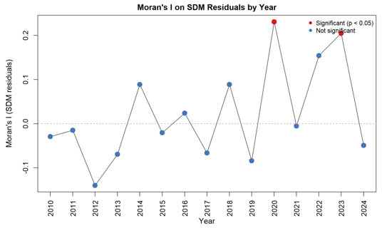
This province-specific instability points to a natural extension of the present design, heterogeneous-coefficient spatial panel models [44], which we take up among the research directions in Section 5. As a final check, Moran's I computed on model residuals is statistically significant in only 2 of 15 years (2020 and 2023), indicating that the model absorbs most cross-sectional dependence; we return to the substantive interpretation of these two exceptions, which bracket Indonesia's most acute COVID-19 disruption, in Section 4.8.
4.7 Shared national trajectory versus genuine diffusion
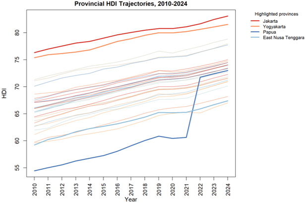
The single most consequential finding concerns how to read Indonesia’s apparent regional convergence in human development: provinces might be truly influencing one another, or simply moving together because they share the same national trajectory, and the answer depends on whether that shared trend is removed first. Estimated without any adjustment, the apparent spillover through HDI itself is large, positive, and highly significant (ρ = 0.473, p < 0.001). Once each province is compared to its peers within the same year, this collapses to −0.08, roughly a sixth of the uncorrected estimate and of opposite sign, and neither asymptotic inference nor the 2,000-replication block bootstrap (Section 4.4) can distinguish it from zero, consistent with a negligible direct HDI-to-HDI channel rather than the large diffusion visible in the uncorrected data. Two independent trend-control strategies, calendar-year controls and within-year peer comparison, converge on the same reversal, and an unrelated software package reproduces the pattern, ruling out a coding error. This is not peculiar to Indonesian HDI data: conflating a shared common factor with genuine cross-sectional dependence is a well-documented source of spurious correlation in panel data [36]. We read this as evidence that HDI’s rise across Indonesian provinces over 2010–2024 is explained mainly by a shared national trajectory, plausibly reflecting national fiscal transfers, macroeconomic growth, or nationwide public-health and education investment [16], rather than province-to-province diffusion. Figure 2 plots each province’s HDI trajectory over 2010–2024 without trend adjustment: nearly every line rises along a similar, roughly parallel path, with the level gaps of Figure 1 carried forward largely unchanged rather than narrowing, the shared national trajectory that cross-sectional demeaning removes.
Figure 2. Provincial Human Development Index (HDI) trajectories, 2010–2024
The same reversal shows up in a second, independent diagnostic. Cross-sectional demeaning flips the Hausman test itself, from failing to reject random effects on the raw data (p = 0.109) to strongly rejecting it once demeaned, a result an independent Python implementation reproduces to three significant figures. The most plausible explanation is that the between-year variation removed by demeaning was largely uncorrelated with unobserved provincial heterogeneity, while the within-year variation that remains, a province’s rank relative to its peers, is more persistent and more clearly correlated with it; consistent with this, the R² of the corresponding non-spatial random-effects regression falls from 0.666 on raw data to 0.133 once demeaned. This is why we retain random effects for our preferred SDM despite the Hausman rejection (Section 3.5) [41]; Table A1 shows the choice makes little practical difference. Failing to separate a shared trend from genuine cross-regional influence risks mistaking a national phenomenon for successful regional diffusion, a lesson that extends to any similarly structured dataset: a moderate number of regions observed over many years, with an outcome rising nationally.
4.8 Substantive interpretation of the robust findings
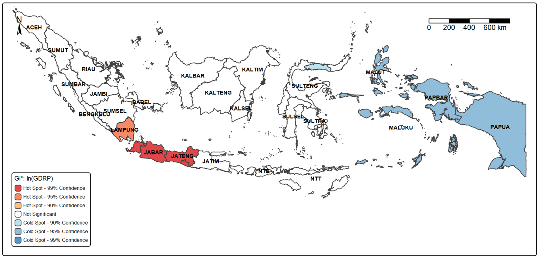
Section 4.7 answers this paper’s central question, whether human development itself spreads across provincial borders. For the most part it does not: once the shared national trend is removed, the direct HDI-to-HDI channel is small and statistically null by both the asymptotic and bootstrap standards of Section 4.4, evidence against a direct diffusion channel rather than a compensatory one. This does not mean cross-provincial influence is absent, only that it does not operate through HDI itself. We now interpret the findings that survive these checks: setting aside the fragile and trend-related estimates, two withstand every check in sign and significance, and a third holds only in the full sample. First, a province’s own GRDP carries a sizeable positive spillover to its neighbours’ HDI, robust to bootstrap resampling and to the choice of spatial weight matrix. This fits a regional-agglomeration interpretation, in which economic activity in one province generates demand, employment, or public-revenue effects extending to proximate provinces, a mechanism formalised in the classic core-periphery account of how increasing returns concentrate activity and propagate benefits to a surrounding region [45], and consistent with evidence that agglomeration economies generate productivity spillovers to neighbouring regions [46]. Figure 3 maps the local Getis–Ord Gi* statistic on ln(GRDP) for 2024, a cross-sectional snapshot rather than a period average like Figure 1, showing a significant economic hot spot centred on Java (West Java, Banten, Jakarta, Central Java, and Yogyakarta at 99 percent confidence, Lampung at 95 percent) and a cold spot across eastern Indonesia, a pattern that lines up with the neighbour-level spillover reported above.
Second, a province’s own health expenditure is negatively and robustly associated with its own HDI, which we do not read as evidence that health spending is harmful. Indonesian provincial and central health allocations are known to include compensatory and equalisation components: a comparable negative association is reported using an entirely different estimator [4], and district-level evidence from North Sumatra finds health expenditure to carry no reliable positive association with HDI once other sectoral spending and poverty are accounted for [47]. This sits awkwardly alongside evidence that life expectancy, HDI’s longevity component, responds positively to health-infrastructure provision elsewhere in Indonesia [24]; the difference is plausibly one of what is held fixed, since that evidence conditions on infrastructure stock rather than the annual expenditure flow we study, and a compensatory rule can raise both spending and infrastructure in lagging provinces while the direct flow-to-level association still comes out negative. The more plausible reading is reverse causality: provinces with lower human development receive larger remedial allocations, or the association reflects confounding correlated with both variables.
Figure 3. Getis–Ord Gi* hot spots for ln(GRDP), 2024
Third, the spillover from neighbouring economic-affairs expenditure is negative and significant in the full sample, but, unlike the two findings above, does not survive the exclusion of a single province: as Section 4.6 details, dropping Papua alone shrinks the coefficient roughly six-fold and raises its p-value from below 0.001 to 0.099, short of the 5 percent level. We therefore report this pattern only tentatively. If it holds, it would be consistent with the classic account of fiscal competition, in which jurisdictions bidding for the same pool of mobile investment or labour adjust their spending in response to a neighbour’s, though we cannot distinguish this from other explanations with the present design [48].
Conspicuously absent are education and social-protection expenditure: neither carries a statistically significant direct or indirect coefficient anywhere in Tables 3 to 5. This null result sits in some tension with evidence that education quality is linked to HDI outcomes elsewhere in Indonesia [25]; a plausible reconciliation is that our covariate measures the scale of education spending rather than its quality or targeting, and if quality rather than volume drives the education component of HDI, a model built on expenditure levels alone would not detect it. We do not treat this absence as evidence that education and social-protection spending are irrelevant to human development; rather, it marks a boundary of what a scale-based expenditure model can identify, and a natural target for future work using spending-quality or targeting measures rather than raw budget totals.
Two further patterns emerged from diagnostics we ran for their own sake rather than to test a hypothesis. Moran’s I computed on raw (unmodelled) HDI levels is significant in every year from 2010 to 2021, but in none from 2022 to 2024, suggesting that the spatial clustering of human development levels across provinces may have weakened in the most recent years, plausibly related to the uneven geography of Indonesia’s post-pandemic recovery and flagged for future research. Separately, residual spatial autocorrelation after modelling is significant specifically in 2020 and 2023 (Figure 4), the years bracketing Indonesia’s most acute COVID-19 disruption, pointing to a structural break in the spatial process during the pandemic that our time-invariant specification does not capture.
Figure 4. Moran's I on model residuals by year
This paper asked whether Indonesia’s regional disparities in human development are narrowing because progress genuinely spreads across provincial borders, or because every province is simply riding the same national trend. Studying all 33 provinces from 2010 to 2024, we separated the shared trend from real cross-province relationships, a distinction that determines the answer. Once it is drawn, the direct channel from one province’s human development to its neighbours’ is small, negatively signed, and statistically null under both inference methods, evidence against direct cross-province diffusion rather than for a compensatory pattern. What spreads more reliably is economic activity: a province’s economic scale (GRDP) carries a positive spillover to its neighbours’ HDI that is robust in sign and significance, though its magnitude (1.2 to 7.7) depends on how a neighbourhood is defined and on the exclusion of individual provinces. A province’s own health expenditure, by contrast, is negatively associated with its own outcomes, which we attribute to compensatory allocation toward lagging provinces rather than a harmful effect of spending. What looks like convergence among neighbours therefore tracks a shared national trajectory more than genuine diffusion, and place-based policy should not presume that human development gains spread automatically to neighbours through that channel.
These findings apply to Indonesia’s 33 provinces over 2010–2024, a period spanning substantial fiscal decentralisation reform and, toward its end, the COVID-19 pandemic. Whether the weakening of spatial clustering we document for 2022–2024 reflects a durable structural shift or a transient pandemic-recovery artefact cannot be determined from the present data, and is a natural direction for future work as more post-pandemic years become available.
For policy, our results offer a cautious lesson rather than a directive. Because the estimated direct spillover from neighbours’ human development is small, negatively signed, and indistinguishable from zero by both asymptotic and bootstrap standards, policies aimed at raising HDI in lagging provinces should not presume that gains will mechanically diffuse to neighbours through that channel. The one robust spillover we identify operates through economic scale, suggesting that regional economic integration, rather than proximity to high-HDI neighbours per se, is the more promising lever for indirect gains, consistent with Indonesia’s 2025–2029 national development plan, which frames strengthened local economic competitiveness rather than proximity-based diffusion as a principal instrument for narrowing regional disparities [49]. Our health-expenditure finding carries a complementary implication: because the negative association is more plausibly compensatory than harmful, it corroborates rather than undermines the plan’s strategy of directing larger transfers to fiscally weaker regions, and evaluations should not mistake that remedial targeting for evidence that health spending fails to work. We are conservative here because our design identifies associations, not causal effects: provincial expenditure is plausibly endogenous to development outcomes, and we lack a credible instrument or exogenous policy variation to sever this link.
Several caveats apply. First, our time-effect control, cross-sectional yearly demeaning, is a deterministic approximation to a formal two-way random-effects specification and, as Section 3.4 details, mechanically induces a small amount of negative cross-sectional dependence among the demeaned variables; we cannot show it is exactly equivalent to a two-way specification for the quasi-maximum-likelihood spatial estimator we use, and though we doubt this dependence is large enough to explain the negative SAR and SEM coefficients, we cannot rule out that it contributes to their sign. Researchers with software supporting genuine two-way random effects for spatial panels, or an interactive fixed-effects estimator that models the common factor directly [37], should treat our approach as second-best. Second, we cannot rule out reverse causality or omitted confounding in the expenditure–HDI relationship. Third, our jackknife shows Papua materially influences several coefficients; we retain it because excluding an outlier would itself bias inference about the disparities the paper studies. Fourth, we do not conduct an out-of-sample validation. Fifth, our expenditure variables are nominal and in levels rather than real, population-adjusted terms; demeaning nets out trends common to all provinces, including inflation, but cannot correct for cross-province differences in population or price levels, which may contribute to our expenditure coefficients. Sixth, our panel holds Indonesia’s geography fixed at 33 units throughout 2010–2024 by construction of the underlying BPS series (Section 3.1), even though the official province count rose over the period; we rely on that series’ boundary treatment rather than re-aggregating, and future work with district-level data could verify it.
Future work could extend this analysis in five directions. Three concern data and identification: an instrumental-variables or dynamic GMM strategy suited to spatial panels to move toward causal identification of the expenditure–HDI relationship; testing whether the apparent 2022–2024 weakening of spatial clustering persists as further post-pandemic data accumulate; and disaggregating the health-expenditure finding by sub-category (curative versus preventive spending) to distinguish a compensatory-allocation explanation from alternatives. Two concern specifications: a heterogeneous-coefficient spatial panel to test whether the province-level instability our jackknife detects reflects genuine coefficient heterogeneity rather than a single outlier; and replacing education and social-protection expenditure scale with measures of spending quality or targeting, which our design cannot distinguish from volume and which Section 4.8 identifies as the likely reason these covariates carry no detectable association with HDI.
The human development and provincial expenditure series analysed here derive from statistics published by Indonesia’s national statistics agency (BPS), and the provincial boundaries used to construct the spatial weight matrix are from the GADM database; both sources are publicly available. The assembled province-year panel and the four R scripts that produce every table and figure, together with the independent cross-check implementation referenced in Sections 4.1 and 4.7, are available from the corresponding author on reasonable request.
|
Gi* |
Getis–Ord local clustering statistic, dimensionless |
|
HDI |
Human Development Index of a province in a given year, dimensionless |
|
I |
identity matrix, dimensionless |
|
k |
number of nearest neighbours defining a province's neighbourhood, dimensionless |
|
N |
number of provinces (33), dimensionless |
|
T |
number of years (15), dimensionless |
|
W |
row-standardised k-nearest-neighbour spatial weight matrix, dimensionless |
|
X |
vector of six covariates: the Gini ratio, the natural logarithms of economic-affairs, health, education, and social-protection expenditure, and the natural logarithm of GRDP; expenditure and GRDP in nominal rupiah |
|
Greek symbols |
|
|
α |
intercept, dimensionless |
|
β |
vector of coefficients on own-province covariates, dimensionless |
|
ε |
idiosyncratic disturbance, dimensionless |
|
θ |
vector of coefficients on spatially lagged covariates, dimensionless |
|
λ |
spatial error coefficient, dimensionless |
|
μ |
province-specific random effect, dimensionless |
|
ρ |
spatial autoregressive coefficient, dimensionless |
|
Subscripts |
|
|
i, j |
province index |
|
t |
year index |
Table A1 reports the full-coefficient transparency check referenced in Section 3.5 and discussed in Section 4.7.
Table A1. Random versus fixed effects, spatial-lag branch
|
Variable |
SDM (RE) |
SDM (FE, lag) |
|
Gini ratio |
1.462 |
1.309 |
|
ln(Economic affairs) |
0.232 |
0.241 |
|
ln(Health) |
−0.424 |
−0.430 |
|
ln(Education) |
−0.045 |
−0.033 |
|
ln(Social protection) |
0.041 |
0.049 |
|
ln(GRDP) |
−3.400 |
−3.828 |
|
W × Gini ratio |
−7.149 |
−6.948 |
|
W × ln(Economic affairs) |
−0.731 |
−0.733 |
|
W × ln(Health) |
0.228 |
0.245 |
|
W × ln(Education) |
0.044 |
0.047 |
|
W × ln(Social protection) |
0.055 |
0.052 |
|
W × ln(GRDP) |
3.809 |
3.831 |
|
ρ (spatial AR) |
−0.079 (p = 0.251) |
−0.102 (p = 0.087) |
[1] United Nations. (2015). Transforming Our World: The 2030 Agenda for Sustainable Development. United Nations, New York. https://digitallibrary.un.org/record/3923923?v=pdf.
[2] Saputra, D.A., Setiawan, D. (2026). Regional revenues and human development index: An empirical evidence from Indonesia. Revista Brasileira de Gestão e Desenvolvimento Regional, 22(1): 1-29. https://doi.org/10.54399/rbgdr.v22i1.7446
[3] Sijabat, R. (2024). Impact of economic growth, village funds, and poverty on human development in Indonesia: An analytical study from 2015 to 2022. International Journal of Advanced and Applied Sciences, 11(3): 238-250. https://doi.org/10.21833/ijaas.2024.03.023
[4] Susilo, Prasetyia, F., Wicesa, N.A., Finuliyah, F. (2026). The impact of fiscal decentralization on human development index convergence in Indonesia: An Arellano-Bond GMM dynamic panel data estimation. Forum for Social Economics, 1-29. https://doi.org/10.1080/07360932.2025.2610937
[5] Sofilda, E., Hamzah, M.Z., Kusairi, S. (2023). Analysis of fiscal decentralisation, human development, and regional economic growth in Indonesia. Cogent Economics & Finance, 11(1): 2220520. https://doi.org/10.1080/23322039.2023.2220520
[6] Aritenang, A.F., Chandramidi, A.N. (2022). The spatial effects of fiscal decentralization on regional convergence: The case of regions in Indonesia. GeoJournal, 88(2): 2011-2030. https://doi.org/10.1007/s10708-022-10724-2
[7] Miranti, R.C., Mendez, C. (2022). Social and economic convergence across districts in Indonesia: A spatial econometric approach. Bulletin of Indonesian Economic Studies, 59(3): 421-445. https://doi.org/10.1080/00074918.2022.2071415
[8] Septiawan, A.R., Handajani, S.S., Martini, T.S. (2018). Spatial Durbin error model for human development index in Province of Central Java. Journal of Physics: Conference Series, 1025: 012107. https://doi.org/10.1088/1742-6596/1025/1/012107
[9] Yulianti, S., Widyanigsih, Y., Nurrohmah, S. (2021). Spatial panel data model on human development index at Central Java. Journal of Physics: Conference Series, 1722(1): 012090. https://doi.org/10.1088/1742-6596/1722/1/012090
[10] Sutaryo, N.A., Arifin, T., Muhtar, N.A., Ekwanto, N.A. (2025). Does government spending really contribute to development: Evidence from Indonesia. International Journal of Monetary Economics and Finance, 18(5): 299-315. https://doi.org/10.1504/ijmef.2025.148855
[11] Sari, V.A., Tiwari, S. (2024). The geography of human capital: Insights from the subnational human capital index in Indonesia. Social Indicators Research, 172(2): 673-702. https://doi.org/10.1007/s11205-024-03322-x
[12] Soejoto, A., Subroto, W.T., Suyanto, Y. (2015). Fiscal decentralization policy in promoting Indonesia human development. International Journal of Economics and Financial Issues, 5(3): 763-771.
[13] Siburian, M.E. (2019). Fiscal decentralization and regional income inequality: Evidence from Indonesia. Applied Economics Letters, 27(17): 1383-1386. https://doi.org/10.1080/13504851.2019.1683139
[14] Yanto, H., Pujiati, A., Handayani, B.D., Ridzuan, A.R., Keshminder, J.S., Rachman, M.A. (2024). Good government governance as a moderator in achieving sustainable development goals in Indonesia. International Journal of Sustainable Development and Planning, 19(2): 715-722. https://doi.org/10.18280/ijsdp.190228
[15] Ernanto, Sriyana, J., Hakim, A., Sidiq, S. (2024). Enhancing human capital in Indonesia: Does economic policy work? International Journal of Sustainable Development and Planning, 19(5): 1963-1969. https://doi.org/10.18280/ijsdp.190535
[16] Thawley, C., Crystallin, M., Verico, K. (2024). Towards a higher growth path for Indonesia. Bulletin of Indonesian Economic Studies, 60(3): 247-282. https://doi.org/10.1080/00074918.2024.2432035
[17] Hamrullah, H., Saudi, N.D.S., Djam’an, F., Hamzah, S. (2026). Spatial spillovers in regional economic inequality: Evidence from macro indicators—Remote sensing in Eastern Indonesia. Economies, 14(4): 109. https://doi.org/10.3390/economies14040109
[18] Ifa, K., Viphindrartin, S., Santoso, E., Priyono, T.H. (2024). Spatial dependence and poverty factors: A study of Pantura regions in East Java Province, Indonesia. Journal of Infrastructure, Policy and Development, 8(7): 4195. https://doi.org/10.24294/jipd.v8i7.4195
[19] Asyahid, E.A., Pekerti, I.S. (2022). Economic impact of natural disasters, spillovers, and role of human development: Case of Indonesia. Letters in Spatial and Resource Sciences, 15(3): 493-506. https://doi.org/10.1007/s12076-022-00307-7
[20] Niranjan, R. (2020). Spatial inequality in human development in India: A case study of Karnataka. Sustainable Futures, 2: 100024. https://doi.org/10.1016/j.sftr.2020.100024
[21] Luo, X., Qin, J., Wan, Q., Jin, G. (2023). Spatial human development index in China: Measurement and interpretation based on Bayesian estimation. International Journal of Environmental Research and Public Health, 20(1): 818. https://doi.org/10.3390/ijerph20010818
[22] Wang, S., Pan, L., Liu, J. (2024). Spatial differences and driving mechanism of carbon-emission-sensitive human development index in Poyang Lake Basin. Resources Science, 46(8): 1620-1635. https://doi.org/10.18402/resci.2024.08.12
[23] Lehnert, M.R., Smirnov, O. (2022). Human development in Morocco: Out-of-sample prediction using spatial econometrics and RandomForest. African Geographical Review, 43(1): 60-79. https://doi.org/10.1080/19376812.2022.2107547
[24] Setyadi, S., Kustanto, A., Widiastuti, A. (2023). Life expectancy in Indonesia: The role of health infrastructure political and socioeconomic status. Iranian Economic Review, 27(3): 965-1005. https://doi.org/10.22059/ier.2023.329904.1007259
[25] Setyaningrum, D. (2024). Quality education and human development index. International Journal of Economic Policy in Emerging Economies, 20(3/4): 304-311. https://doi.org/10.1504/ijepee.2024.142467
[26] Suharyono, Digdowiseiso, K., Sugiyanto, E., Zulmasyhur. (2018). Causality on the growth-governance-fiscal decentralization nexus: An analysis of time series in Indonesia. Journal of Applied Economic Sciences, 13(7(61)): 1854-1863.
[27] Aji, P., Wibisono, I.D., Suryahadi, A. (2021). Income, inequality and poverty convergence at the local government level in decentralized Indonesia. Journal of Southeast Asian Economies, 38(3): 375-400. https://doi.org/10.1355/ae38-3f
[28] LeSage, J., Pace, R.K. (2009). Introduction to Spatial Econometrics. Chapman and Hall/CRC. https://doi.org/10.1201/9781420064254
[29] Pham, T.T., Vu, T.T., Luu, H.D., et al. (2026). Correcting scale mismatch in sustainability indicators: Spatial decomposition evidence from Vietnam’s provincial indicator system. Environmental Challenges, 24: 101549. https://doi.org/10.1016/j.envc.2026.101549
[30] Anselin, L. (1988). Spatial Econometrics: Methods and Models. Springer Netherlands. https://doi.org/10.1007/978-94-015-7799-1
[31] Elhorst, J.P. (2014). Spatial Econometrics. Springer Berlin Heidelberg. https://doi.org/10.1007/978-3-642-40340-8
[32] Lee, L., Yu, J. (2010). Some recent developments in spatial panel data models. Regional Science and Urban Economics, 40(5): 255-271. https://doi.org/10.1016/j.regsciurbeco.2009.09.002
[33] Elhorst, J.P. (2010). Applied spatial econometrics: Raising the bar. Spatial Economic Analysis, 5(1): 9-28. https://doi.org/10.1080/17421770903541772
[34] Millo, G., Piras, G. (2012). splm: Spatial panel data models in R. Journal of Statistical Software, 47(1): 1-38. https://doi.org/10.18637/jss.v047.i01
[35] Baltagi, B.H. (2013). Econometric Analysis of Panel Data, 5th ed. Wiley, Chichester.
[36] Pesaran, M.H., Tosetti, E. (2011). Large panels with common factors and spatial correlation. Journal of Econometrics, 161(2): 182-202. https://doi.org/10.1016/j.jeconom.2010.12.003
[37] Bai, J. (2009). Panel data models with interactive effects. Econometrica, 77(4): 1229-1279. https://doi.org/10.3982/ECTA6135
[38] Anselin, L., Bera, A.K., Florax, R., Yoon, M.J. (1996). Simple diagnostic tests for spatial dependence. Regional Science and Urban Economics, 26(1): 77-104. https://doi.org/10.1016/0166-0462(95)02111-6
[39] Burridge, P. (1981). Testing for a common factor in a spatial autoregression model. Environment and Planning A, 13(7): 795-800. https://doi.org/10.1068/a130795
[40] Mutl, J., Pfaffermayr, M. (2011). The Hausman test in a Cliff and Ord panel model. The Econometrics Journal, 14(1): 48-76. https://doi.org/10.1111/j.1368-423x.2010.00325.x
[41] Lee, L., Yu, J. (2010). Estimation of spatial autoregressive panel data models with fixed effects. Journal of Econometrics, 154(2): 165-185. https://doi.org/10.1016/j.jeconom.2009.08.001
[42] Wooldridge, J.M. (2010). Econometric Analysis of Cross Section and Panel Data, 2nd ed. MIT Press, Cambridge, MA.
[43] Baltagi, B.H., Song, S.H., Koh, W. (2003). Testing panel data regression models with spatial error correlation. Journal of Econometrics, 117(1): 123-150. https://doi.org/10.1016/s0304-4076(03)00120-9
[44] Chih, Y.Y., LeSage, J.P. (2021). Heterogeneous coefficient spatial regression panel models. In Handbook of Regional Science, pp. 2219-2236. Springer Berlin Heidelberg. https://doi.org/10.1007/978-3-662-60723-7_121
[45] Krugman, P. (1991). Increasing returns and economic geography. Journal of Political Economy, 99(3): 483-499. https://doi.org/10.1086/261763
[46] Li, J., Jin, H., A, L., Qiu, Y. (2026). Digital economy and green TFP in manufacturing: Heterogeneous, agglomeration and spillover effects revisited. Journal of Economic Studies, 1-17. https://doi.org/10.1108/jes-02-2025-0087
[47] Pratomo, W.A., Asmalidar, Suprayitno, A. (2026). Sectoral public spending, human development, and income inequality in North Sumatra Province: District-level evidence from Indonesia. Public and Municipal Finance, 15(2): 133-147. https://doi.org/10.21511/pmf.15(2).2026.11
[48] Keen, M., Marchand, M. (1997). Fiscal competition and the pattern of public spending. Journal of Public Economics, 66(1): 33-53. https://doi.org/10.1016/s0047-2727(97)00035-2
[49] Ministry of National Development Planning/Bappenas. (2025). Rencana Pembangunan Jangka Menengah Nasional (RPJMN) 2025-2029. Government of Indonesia, Jakarta. https://perpustakaan.bappenas.go.id/e-library/file_upload/koleksi/dokumenbappenas/konten/Dokumen%202025/Konten/%7BDigital%7D%20Ringkasan%20RPJMN%20Tahun%202025-2029.pdf.