Redouane Mouti | Hamza El Baraka*![]() | Khalil Bourouis
| Khalil Bourouis![]() | Mohamed Rakiai | Abdellali Fadlallah
| Mohamed Rakiai | Abdellali Fadlallah
© 2025 The authors. This article is published by IIETA and is licensed under the CC BY 4.0 license (http://creativecommons.org/licenses/by/4.0/).
OPEN ACCESS
Monitoring the level of tax pressure, evolution, and its extent constantly attracts the attention of public authorities because of its direct impact on economic performance. Thus, for several years, numerous studies have attempted to define evaluation standards, subsequently used to analyze the optimal level of tax pressure, its evolution and its effects on economic growth. The objective of this study is therefore to empirically evaluate the fiscal potential using the tax effort approach to determine the extent of the budgetary margins available in Morocco. In our study, we used three panel data regressions from 46 developing countries for the period spanning 1990 to 2022. According to our results, we identified an estimated under pressure of 2.9% and which changes by 1.7% on average for the three models. Thus, the subsequent reforms of the tax system have not made it possible to strengthen the effective levy to a level beyond its capacity.
tax effort, tax capacity, panel data, Hausman test, dynamic model
Nowadays, the importance of analyzing the structural level of tax pressure remains a major concern for all economic agents. Consequently, monitoring its evolution consistently draws the attention of budgetary authorities, particularly in developing countries, due to its direct link with key macroeconomic performances. In this regard, an in-depth analysis of the optimal level of tax pressure and its implications helps guide strategic decisions aimed at promoting sustainable and balanced economic development.
In Morocco, the contribution of tax revenues to budgetary revenues appears like that observed in countries with modern tax systems. Recent fiscal policy frameworks aim to support economic activity, diversify financing sources, and promote social development by optimizing tax revenues, expanding the taxable base, and controlling tax expenditures. Thus, the primary objectives focus on the sustainability of fiscal policy, broadening financing sources for the budgetary economy, fostering growth and social development through optimizing tax revenues by expanding the tax base, rationalizing tax expenditures, and maintaining oversight.
It is worth noting that international experience with tax pressure over the past decades has shown that excessive tax pressure can negatively impact a country's economic performance. The potential level of tax pressure, therefore, refers to the value that simultaneously ensures internal economic stability and the external viability of fiscal effort, with a key focus on the study of the international tax ratio While previous literature, including the seminal work of Lotz and Morss [1], has explored the concept of fiscal effort, few studies have assessed this in the context of Morocco using dynamic econometric techniques [1].
This study addresses this gap by evaluating Morocco’s fiscal potential through the fiscal effort approach, employing a dynamic panel data model using the Generalized Method of Moments (GMM). By benchmarking Morocco against a sample of 45 other developing countries over the period 1990–2022, we provide new empirical evidence on Morocco's relative position in mobilizing budgetary resources.
The objective of this study is to evaluate Morocco’s fiscal potential using the fiscal effort approach to analyze its impact on optimizing the State's budgetary resources. Specifically, by assessing fiscal effort, we aim to determine whether Morocco is fully exploiting its revenue collection potential, considering its economic structure and public policies. More specifically, our study will compare Morocco's fiscal potential to that of its main partner and competitor countries. This approach allows us to identify to what extent Morocco is utilizing its tax collection capacity, given its structural and institutional characteristics. The findings offer critical insights for fiscal policy design, helping guide reforms toward more effective and equitable revenue mobilization in a regional and international context.
The concepts of tax pressure, fiscal potential, and tax effort are central to the analysis of public finance systems and the performance of tax policy. Tax pressure typically refers to the ratio of tax revenue to GDP, representing the actual burden of taxation on an economy. Fiscal potential, on the other hand, denotes the maximum revenue a government could feasibly collect based on its economic structure and administrative capacity. Tax effort is the ratio of actual tax revenue to estimated fiscal potential and reflects the intensity of tax collection in relation to what is economically possible [2, 3].
A variety of theoretical and empirical frameworks have been developed to measure fiscal potential and effort. Macroeconomic approaches focus on aggregate indicators such as GDP per capita, trade openness, and the size of the informal sector to estimate potential tax capacity. These models are useful for cross-country comparisons but often neglect structural heterogeneity within countries, especially in contexts with high regional disparities or evolving informal economies [4]. In contrast, microeconomic approaches disaggregate the tax base by incorporating household consumption, sectoral value-added, and firm-level dynamics, enabling a more granular understanding of local fiscal capacities. However, these models are data-intensive and often limited by the availability of detailed microdata [5-8].
To complement these traditional approaches, researchers have proposed composite fiscal performance indices that aggregate multiple fiscal and institutional indicators to provide a more comprehensive assessment. While such indices facilitate cross-country benchmarking, they often fail to capture underlying structural differences, thereby limiting their policy applicability in heterogeneous economic environments [9]. Chelliah et al. [2] proposed one of the earliest empirical frameworks for measuring tax effort by comparing actual tax ratios to predicted values based on structural economic variables.
Empirical studies in this field can be broadly categorized based on their methodological orientation. Non-structural (statistical) methods rely on time-series techniques to extract long-term trends in tax pressure, such as the Hodrick–Prescott (HP) filter, which decomposes revenue series into trend and cyclical components [10]. These models treat time as a driving variable and are particularly useful for identifying deviations from long-run fiscal norms. Alternatively, structural approaches are grounded in economic theory and often involve modeling fiscal capacity using production functions that relate output to labor, capital, and technology. These models explore how institutional factors such as wage-setting, tax administration, and capital returns shape tax collection efficiency [11].
Additionally, composite index approaches use multivariate statistical techniques such as Principal Component Analysis (PCA) to construct synthetic measures of tax performance. These methods allow for the integration of both economic and institutional variables, providing a more multidimensional view of tax effort and efficiency. Pessino and Fenochietto [7], for instance, applied such an approach to compare tax performance across countries with similar structures but varying tax burdens [12].
A wide range of empirical studies supports the use of cross-sectional and panel data models to estimate fiscal potential and tax effort. Early work by Lotz and Morss [1], Bahl [10], and Tanzi and Zee [13] used cross-sectional regressions to identify key predictors of tax capacity [13-18]. More recent studies have utilized panel regressions with fixed or random effects to account for temporal and country-specific heterogeneity [14, 19]. Meanwhile, hybrid models incorporating institutional quality, governance, and administrative capacity offer more realistic estimations of tax effort, particularly in developing and emerging economies [3].
The concept of fiscal effort offers a crucial measure to evaluate the extent to which countries are leveraging their potential for public revenue generation. To do so, it is essential to distinguish between the share of public resources dictated by intrinsic structural factors and the share influenced by economic policy and state action in general. This distinction provides a better understanding of how political decisions and strategic choices impact the mobilization of public revenues, enabling the identification of levers to optimize tax revenues.
The tax rate of an economy $i$ at a given date $(t)$, denoted as $T P_{i, t}$, results from the interaction between the fiscal potential of that economy at the given date $\left(P F_{i, t}\right)$ and the fiscal effort exerted, represented by $E F_{i, t}$, expressed as:
$T P_{i, j}=f\left(P F_{i, j}, E F_{i, j}\right)=P F_{i, t}.+E F_{i, t}$
This effort can be considered an additive variable relative to fiscal potential, reflecting the intensity of efforts by the state to collect tax revenues on the one hand and to identify opportunities for improvement and analyze efficiency in mobilizing public resources on the other hand.
We also adopt, based on the stochastic frontier model by Kumbhakar et al. [17], a second specification of this measure, combining two aspects of inefficiency: one that is persistent and stable over time, and another that evolves over time [17]. For reference, this second baseline model is expressed as follows.
$Y=\alpha+\beta^{\prime *} X i t+\mu_{\mathrm{i}}+\vartheta i t-\omega i-\mu_{\mathrm{it}}$
where, $Y=L n(T P F)=L n(\mathrm{RF} / \mathrm{GDP})$ represents the logarithm of effective tax revenues as a proportion of GDP, i.e., the logarithm of the tax pressure rate TPF, with RF denoting effective tax revenues and RF/GDP the tax pressure rate. X denotes the vector of logarithms of variables representing explanatory factors (structural factors), $\mu \mathrm{i}$ captures unobserved time-invariant variables, specifically omitted structural factors, vit represents time-varying error terms approximating heterogeneity among countries, particularly differences in tax culture and morale, $\omega \mathrm{i}$ is the time-invariant inefficiency term related to fiscal policy measures such as tax laws and the organization of domestic tax services, while $\mu$ it is the timevarying inefficiency term reflecting the performance of the tax administration.
These two inefficiency terms allow for the evaluation of fiscal effort stemming from political decisions, the tax administration's performance, and the overall resulting fiscal effort [15]. The model estimation follows the three-step procedure proposed by Kumbhakar et al. [17]. This procedure involves rewriting the model as follows:
$\operatorname{Ln}(T P F) i t=\alpha^*+\beta^{\prime *} X i t+\mu_{\mathrm{i}}+\vartheta i t$ (1)
where,
$$
\begin{array}{cc}
\alpha *=\alpha-E(\omega i)-E(\mu i t) & (*) \\
\epsilon i t=\vartheta i t-\mu i t+E(\mu i t) & (* *) \\
\alpha i=u i-\omega i+E(\omega i) & (* * *)
\end{array}
$$
This step involves regressing Eq. (1) specified as a panel data model. This regression provides parameter estimates $\beta$ (for $j=1, \ldots, 5$ ) as well as values for $\alpha_i$ and $\epsilon_{i t .}$.
Here, the time-varying inefficiency term $\mu_{i t}$ is estimated using equation (**), based on the estimated value of $\epsilon_{i t}$ from the first step and assuming $v_{i t}$ follows a normal distribution with zero mean and variance $\left(v_{i t} \sim N\left(0, \sigma^2\right)\right)$ and $\mu_{i t}$ follows a half-normal distribution $\left(\mu_{i t} \sim N+\left(0, \sigma^2\right)\right)$. Equation (**) is estimated using a standard stochastic frontier model. The method proposed by Jondrow et al. [16] is then applied to determine the conditional distribution of $\mu_{i t}$ given $\epsilon_{i t}$, enabling an estimate of $\mu_{i t}$. From this estimate, the time-varying fiscal effort $(E F V)$ is calculated as: $E F V_{i t}=\exp (-\mu i t$ Estimated $)$.
This step estimates the time-invariant inefficiency term $\omega_i$ using equation (***) following the same approach as Step 2. It relies on the estimated value of $\alpha_{\mathrm{i}}$, assuming $\mu_{\mathrm{i}}$ follows a normal distribution $\left(\mu_{\mathrm{i}} \sim \mathrm{N}\left(0, \sigma^2\right)\right)$ and $\omega_{\mathrm{i}}$ follows a half-normal distribution $\left(\omega_{\mathrm{i}} \sim \mathrm{N}+\left(0, \sigma^2\right)\right)$. The time-invariant fiscal effort (EFI), i.e., the persistent effort, is calculated as:
$E F I i=\exp (-\omega i$ estimated $)$.
Finally, the overall fiscal effort (EFG) of country $i$ at date $t$ is determined as the product of EFV and EFI is presented as:
$E F G_{\mathrm{it}}=E F V_{\mathrm{it}} \times E F I_{\mathrm{i}}$
In our study, the method adopted to determine fiscal effort is based on estimating an explanatory equation for the tax collection rate as a function of relevant variables over a broad sample of countries and a significant period. We use panel data from 46 developing countries for the period from 1990 to 2022. This approach captures both inter-temporal and cross-country variability while controlling for time-invariant unobserved differences at the country level using random country effects [17]. This helps account for unobserved heterogeneity that may influence tax collection levels.
Using panel data over an extended period and a large sample of countries provides robust estimates of fiscal effort, accounting for both temporal and cross-sectional variations. This offers a more comprehensive perspective on fiscal dynamics in developing countries and helps identify key determinants of fiscal effort, such as economic, institutional, and political characteristics [18]. Additionally, the multidimensional econometric approach used effectively controls unobserved factors that could influence tax collection levels, ensuring the validity and reliability of the results obtained.
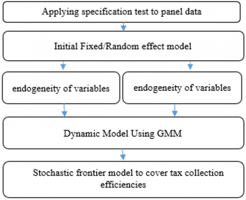
The database used for this study comprises the main explanatory variables of tax pressure (TP), along with temporal (years) and spatial (countries) references. These variables were selected based on the criteria outlined previously. The data were sourced from well-regarded and reliable institutions, including the World Bank (WDI), the IMF, and the OECD. This choice of sources enhances the credibility and quality of the data used in the analysis (Figure 1).
Figure 1. Econometric modelling process
The descriptive statistics (Table 1) reveal key patterns in the dataset. Tax pressure averages 25% of GDP, but with a lower median (19%), indicating that a few high-tax countries raise the overall mean. Inflation is moderate (around 3.5%) but varies significantly across countries. Trade coverage rates are stable and below 1, suggesting most countries import more than they export. Budget balances are consistently positive, showing fiscal surpluses. Investment levels (GFCF) are high and stable across the sample. Productivity varies widely, with some countries showing much higher output per worker.
Table 1. Descriptive statistics
|
Variables |
Mean |
Median |
Stand. Dev. |
Min |
Max |
|
PF (Tax revenue as % of GDP) |
0.25 |
0.19 |
0.03 |
0.18 |
0.28 |
|
Inflation |
3.48 |
3.52 |
2.29 |
0.91 |
11.56 |
|
Coverage rate |
0.76 |
0.75 |
0.05 |
0.63 |
0.95 |
|
Budget balance (% of GDP) |
4.25 |
4.26 |
1.03 |
3.21 |
12.23 |
|
Gross Fixed Capital Formation (% of GDP) |
0.26 |
0.27 |
0.02 |
0.24 |
0.25 |
|
Productivity (constant 2014 USD) |
2561 |
2379 |
592.15 |
1621 |
3456 |
Source: Authors Construction
The data reflect moderate heterogeneity across countries, justifying further analysis of the determinants of tax pressure.
The variables employed in our analysis are primarily structural, meaning they are intrinsically linked to the economic, social, and institutional characteristics of the countries.
Since our econometric model relies on empirical estimates, it is crucial to apply logarithmic transformation during regression to prevent potential bias in the results.
This logarithmic transformation stabilizes data variance and makes the estimated coefficients more interpretable, particularly for variables exhibiting significant discrepancies.
The model we will estimate is as follows:
$\begin{gathered}(T P / G D P)_{i t}=\alpha_i+\beta_{1 t} * G D P C s_{i t}+\beta_{2 t} * T C_{i t}+\beta_{3 t} * \\ P C I_{i t}+\beta_{4 t} * G F C F_{i t}+\beta_{5 t} * S B_{i t}+\varepsilon_{i t}\end{gathered}$
where,
GDP: Economic growth.
TCO: Coverage rate (as a % of GDP), denoted as (TP/GDP) in the model.
PCI: Consumer Price Index.
GDPC: GDP per capita.
GFCF: Gross Fixed Capital Formation.
SB: Budget balance.
According to Table A1, there is a correlation between the explanatory variables and the dependent variable. More specifically, there is a moderate negative correlation between tax pressure (the Tax Revenue/GDP Ratio) and the coverage rate (the ratio between exports and imports). Additionally, a weak positive correlation is observed between GDP per capita and the Tax Revenue/GDP Ratio, whereas there is a negative correlation with investment.
The study relies on multidimensional econometric methods, primarily based on panel data, which allow capturing both time variations and variations across different units of observation, such as countries. These methods consider random country effects, which capture unobserved heterogeneity that may be constant over time. One of the first tests conducted for panel data estimation is the Hausman specification test, which aims to evaluate the appropriateness of choosing between a fixed-effects model and a random-effects model.
From a practical standpoint, the fixed-effects model is often preferred because it effectively controls individual effects that are constant over time. However, it is costly in terms of degrees of freedom, which may limit its ability to detect significant relationships. On the other hand, the assumption of the random-effects model, which posits that there is no correlation between individual effects and other regressors, is often poorly justified in many empirical contexts. Therefore, the Hausman specification test is an essential tool in econometrics for distinguishing between fixed-effects and random-effects models, helping researchers choose the most appropriate model for their data and obtain reliable and meaningful results.
5.1 Fixed and random effects models
The use of fixed effects in econometric analysis assumes that there is a specific fixed effect for everyone, such as a country in the case of a comparative cross-country study. This approach accounts for systematic differences between the units of observation, but it limits the variability of errors to the residuals, meaning the errors are homoscedastic. However, this method has its limitations, particularly in not exhaustively modeling the variability of fixed effects across units of observation.
Conversely, the random effects method extends the fixed effects approach by assuming that the specific effects $\alpha_i$ follow a statistical distribution. Unlike the fixed effects approach, this method allows for modeling the variability of specific effects across different units of observation, providing greater flexibility to capture the diversity of behaviors among individuals or groups. This approach also recognizes that specific effects may vary from one observation to another, allowing for a better adaptation to the nuances and variations in the data $\left(\alpha i=\alpha+\mu_i\right.$ with $\left.\mu_i \sim i i d\right)$.
The panel data used to construct the fiscal potential estimation model is based on the fixed effect generated by the choice of this panel. Using the Hausman test, we initially reject the null hypothesis because the test is significant at the $5 \%$ threshold. This means there is a correlation between individual effects and the explanatory variables. Consequently, we opt for the random effects model, which is globally significant with a p-value below $5 \%$ according to the Fisher test. However, the variable SB is not significant, as shown in Table 2.
Table 2. Initial model
|
Coefficients |
Estimate |
Std. Error |
Z-Value |
Pr(>|z|) |
|
GDPC |
-0.13458044 |
0.00013128 |
-4.4213 |
1.844e-05 *** |
|
TCO |
-0.11368222 |
0.00017098 |
-3.9900 |
0.0001019 *** |
|
GFCF |
0.33009460 |
0.04703508 |
4.9770 |
1.710e-06 *** |
|
INF |
0.26565163 |
0.01457522 |
7.5232 |
4.156e-12 *** |
|
SB |
0. 13449282 |
0.15167931 |
0.0626 |
0.95010 |
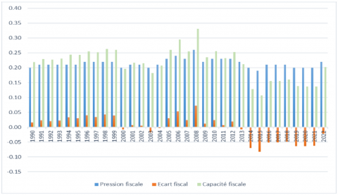
Figure 2. Fiscal potential evolution for the first model
Source: Authors Constructions
Table 2 shows that tax effort is significantly influenced by several factors. GDP per capita has a negative effect, meaning that as income rises, tax effort decreases, due to inefficiencies or regressive taxation. The trade coverage ratio also negatively impacts tax effort, suggesting that greater trade openness may reduce the domestic tax base. Conversely, higher investment (gross fixed capital formation) positively boosts tax effort by expanding the taxable base. Inflation similarly has a positive effect, increasing nominal tax revenues in the short term. The budget balance, however, does not significantly affect tax effort, indicating its complex and indirect relationship with tax collection intensity.
The coefficient of determination $\mathrm{R}^2$, which is approximately $57 \%$ and remains stable after adjustment, indicates that the model is robust for estimating tax pressure. This means that $57 \%$ of the variability in tax pressure can be explained by the structural variables included in the model.
The estimation of fiscal potential, which aims to measure the impact of structural factors on tax pressure, reveals valuable information about the determinants of fiscal policy. In the presented analysis, the results indicate that variables such as GDP per capita and the trade coverage ratio have a negative and significant influence on tax pressure.
Figure 2 shows that the tax pressure remained stable between 0.18 and 0.22 throughout the 1990s and early 2000s. A peak occurred around 2007-2008, reaching approximately 0.25, indicating stronger tax collection during this period. From around 2011 onward, the tax pressure fluctuated slightly but mostly stayed above 0.18. From 1990 to 2008, the fiscal gap remained close to zero, suggesting a minimal difference between actual tax revenue and potential tax capacity. However, after 2011, noticeable negative spikes emerged, with the gap reaching approximately -0.08 around 2015-2017. These negative values indicate that fiscal performance fell below the country’s estimated capacity during these years, reflecting underperformance in revenue mobilization.
Fiscal capacity exhibited a general upward trend from 1990 to around 2008, peaking sharply between 2007 and 2008 (approximately 0.32 to 0.35). This suggests that Morocco’s ability to generate tax revenue improved significantly during this period. However, after 2008, fiscal capacity declined steadily until around 2017, stabilizing afterward at a level lower than its peak years. Fiscal capacity experienced strong growth until around 2008, likely due to economic expansion or reforms that broadened the tax base. During this time, tax pressure also increased, though not as sharp as fiscal capacity, resulting in a small positive (or near-zero) fiscal gap. This alignment indicates that tax collection was relatively efficient compared to the country’s revenue potential.
After 2011, fiscal capacity decreased while tax pressure remained stable, leading to a negative fiscal gap.
This finding suggests that higher income levels per capita, a more dynamic economy with lower inflation and higher trade coverage ratio are associated with lower tax pressure.
The residual tests indicate the presence of heteroscedasticity and autocorrelation, even though they are normally distributed, as confirmed by the Ljung-Box test, the ADF test, and the ARCH test.
The introduction of the logarithmic transformation (LOG) on each variable helped to harmonize the series. By opting for the fixed-effects model following the PLM regression of $\operatorname{LOG}(P F)$ on $\operatorname{LOG}\left(X_{\mathrm{it}}\right)$, the $\mathrm{R}^2$ decrelased to 36%, and the coefficients of LOG(TCO) and FBCF became insignificant (FBCF was not logged due to the presence of negative values, as indicated in the appendix Table A1, Figures A1 and A2).
The residual tests confirm that the errors are now normally distributed, the issue of heteroscedasticity has been resolved, but the problem of autocorrelation persists.
From this model, we can deduce Morocco's fiscal effort, which is obtained by subtracting the actual tax revenue from its fiscal potential. This result is illustrated in Figure 1.
5.2 Dynamic model using GMM
The model faces two major issues: endogeneity of variables and the correlation between the lagged endogenous variable and residuals. Since any convergence model is inherently dynamic, it introduces endogeneity within the explanatory variables. To address these issues, dynamic models are estimated in first differences using the GMM [19]. To operate the dynamic model, we rely on GMM estimation. The results are as follows:
• One-Step GMM Model:
$\begin{gathered}\operatorname{LOG}(P F t)=0.78 . \operatorname{LOG}\left(P F_{t-1}-\right. 0.25 . \operatorname{DIF}(\operatorname{LOG}(P I B))-0.161 \cdot \operatorname{LOG}(I P C)+0.101 \cdot \operatorname{DIF}(\operatorname{LOG}(S B))+0.0036 \cdot \operatorname{DIF}(I N F)+0.61 \cdot \operatorname{DIF}(F B C F)\end{gathered}$
Significance: All coefficients are significant at the 10% threshold.
Residual Tests: These confirm the absence of autocorrelation and heteroscedasticity.
Model Performance: The GMM results are like those from the dynamic fixed-effects model, confirming the robustness of the results.
• Two-Step GMM Model:
In the two-step model, the parameters become non-significant, which impacts the overall reliability of the model.
The one-step GMM model is retained as it satisfies all necessary statistical tests and provides reliable estimates.
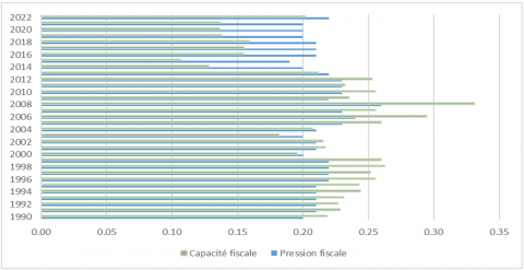
Figure 3 compares two key indicators, Fiscal Capacity and Fiscal Pressure, from 1990 to 2022. Fiscal Capacity represents the government’s potential to generate tax revenue, while Fiscal Pressure reflects the actual tax burden on the economy.
Figure 3. Fiscal effort evolution in Morocco according to the selected model
Over time, both indicators fluctuate, but Fiscal Capacity exceeds Fiscal Pressure, suggesting that the government’s revenue potential often outpaces the real tax burden. In recent years (2020–2022), Fiscal Pressure has remained stable or slightly increased, while Fiscal Capacity dipped in 2020 before recovering by 2022. A notable peak occurred in 2008, when Fiscal Capacity surged above 0.30, signaling a strong revenue-generation potential, whereas Fiscal Pressure stayed steady, mostly below 0.25.
The persistent gap between the two indicators implies that, in many years, the government could enhance tax collection without significantly raising the actual burden on the economy.
5.3 Stochastic Frontier model
From a methodological perspective, fiscal potential, also referred to as the fiscal frontier, represents at any time $t$ the maximum amount of tax revenue (expressed as a percentage of GDP) that can be estimated using an econometric model. This model establishes a correlation between the tax pressure rate and various variables that reflect the structural factors of the economy. Empirical studies have identified three main econometric methods. The stochastic frontier models are based on the principle of technical efficiency, if a country's tax revenues fall below the fiscal frontier due to inefficiencies in the tax collection process. The results obtained are as follows (Table 3):
Table 3. Stochastic model results
|
Dependent Variable: PF |
||
|
Explanatory Variables |
Coefficients |
P-Value |
|
GDPC |
0.245587 |
0.00000000000000022 *** |
|
INF |
-0.105211 |
0.000000000006829 *** |
|
GFCF |
0.070055 |
0.007755 ** |
|
SB |
0.113251 |
0.000009642831849 *** |
|
TCO |
0.123951 |
0.292012 |
|
Fisher |
91.34551 |
0.000000000000000222 *** |
The estimation results indicate that all explanatory variables exhibit the expected signs in line with the literature. Specifically, the relationship between the tax pressure rate and per capita GDP is positive and statistically significant at the 1% level. A 1% increase in per capita GDP leads to a 0.24% rise in the tax pressure rate. Furthermore, the relationships between public investment, the budget balance, and the tax pressure rate are positive and significant at the 5% and 1% levels, respectively. An increase of 1% in the shares of these two sectors results in an improvement in the tax pressure rate by 0.07% and 0.11%, respectively.
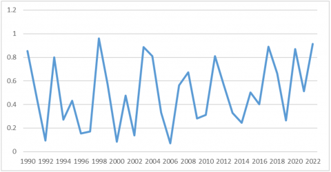
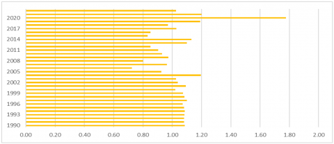
Figure 4 illustrates the evolution of Morocco’s tax effort from 1990 to 2020, as estimated by a specific analytical model. The tax effort index provides insight into how effectively Morocco has mobilized tax revenues relative to its economic potential. An index value of 1.0 typically indicates that the country is collecting taxes in line with its estimated capacity, while values above or below this benchmark suggest overperformance or underperformance, respectively.
Figure 4. Evolution of tax effort in Morocco according to the model used
During the early years of the period analyzed, particularly from 1990 to 2002, Morocco’s tax effort remained stable and consistently close to the benchmark value of 1.0. This indicates a balanced alignment between tax revenue collection and economic potential. In 2005, Morocco achieved a tax effort of exactly 1.0, marking a year where tax revenue collection precisely met its estimated potential. However, following this period, the country experienced a gradual decline in tax effort, reaching its lowest levels between 2008 and 2014, with some years, such as 2011, showing a noticeable dip below 0.7. This decline may reflect policy shifts, economic challenges, or inefficiencies in tax administration during that time.
From 2014 onward, a modest recovery in tax effort is observed, culminating in a dramatic increase in 2020, where the index soared well above 1.8. This exceptional rise suggests a significant and temporary intensification of tax mobilization efforts. It may be linked to emergency fiscal measures implemented in response to the COVID-19 pandemic, administrative improvements, or extraordinary revenue sources. Overall, the figure reveals a fluctuating yet responsive tax system, with periods of both underperformance and strong recovery, reflecting the broader fiscal and economic context of the country.
Trade policy has a favorable but non-significant effect on the tax pressure rate. A 1% increase in international trade translates into a 0.12% improvement in the tax pressure rate. Conversely, as widely emphasized in literature, the negative sign of the coefficient for inflation indicates that this variable does not contribute to increasing tax revenues. Specifically, a 1% increase in the share of value added from the agricultural sector results in a 0.12% decrease in the tax pressure rate.
As illustrated in Figure 5, the fiscal effort, derived from the difference between fiscal potential and actual tax collection, results from the model, yielding an estimated average under-collection or shortfall of 2.8%, which evolves to an average of 1.7% across the three models. Thus, successive reforms of the tax system have not succeeded in increasing actual tax collection beyond its capacity.
Figure 5. Evolution of tax effort in Morocco according to the model used
The tax system represents one of the key determinants of the structural performance of each country's economic policy. This policy involves using certain budgetary instruments, such as direct or indirect taxes, to finance economic activity. Thus, like political actions, fiscal policy reflects political orientations and an analysis of the nation's economic and social situation.
According to the experience of advanced countries, fiscal policy plays a central role in economic and social development [20]. For developing countries, whose tax revenues are the main sources of financing, mobilizing these revenues remains one of the most pressing issues for several reasons. On the one hand, these countries need to finance significant expenditures for sustainable development. On the other hand, in a context marked by rising public debt, the collection of taxes represents a central tool for financing the economy.
International experience in fiscal policy over the past decades has shown that high tax pressure can have negative consequences on a country's economic performance. This is why most economists emphasize the importance and necessity for countries to implement fiscal policies capable of mitigating, or even eliminating, the unfavorable repercussions of high tax pressure. The debate, both theoretically and empirically, then focuses on tax pressure and the choice of an optimal tax level.
More concretely, higher tax pressure relative to key partners leads to an increase in the relative prices of domestic goods compared to foreign goods. As a result, there is a loss of competitiveness of domestic goods and a deterioration in competitive positioning. Such a situation can be acceptable as long as the current account deficit remains sustainable.
According to our results, the annual evolution of the fiscal potential in geometric average for Morocco during the study period is 1.7%, indicating a level of actual tax collection lower than the tax pressure of comparison countries, leading to a budgetary shortfall of 2.8%. Thus, according to the fiscal effort criterion, Morocco’s public resource space has been underutilized, reflecting a fiscal expenditure that impacts economic growth.
Table A1. Correlation matrix
|
|
PF |
INF |
TCO |
SB |
GFCF |
PROD |
|
PF |
1.00 |
|
|
|
|
|
|
INF |
-0.22 |
1.00 |
|
|
|
|
|
TCO |
0.09 |
0.31 |
1.00 |
|
|
|
|
SB |
-0.51 |
-0.15 |
0.29 |
1.00 |
|
|
|
GFCF |
-0.28 |
-0.36 |
-0.65 |
0.27 |
1.00 |
|
|
PROD |
0.0015 |
-0.44 |
-0.63 |
-0.11 |
0.78 |
1.00 |
Figure A1. Tax revenue as a percentage of GDP in Morocco, 2000–2022
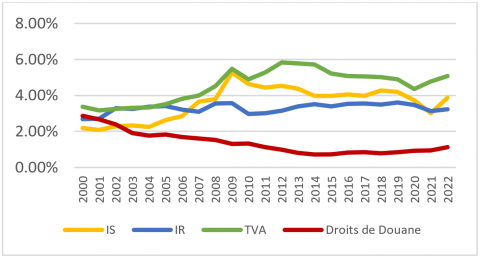
Figure A2. Tax revenue as a percentage of GDP in Morocco by type of tax, 2000–2022
[1] Lotz, J.R., Morss, E.R. (1967). Measuring “tax effort” in developing countries. IMF Staff Papers, 14(3): 478-499. https://doi.org/10.2307/3866266
[2] Chelliah, R.J., Baas, H.J., Kelly, M.R. (1975). Tax ratios and tax effort in developing countries, 1969-1971. IMF Staff Papers, 22(1): 187-205. https://doi.org/10.2307/3866592
[3] Gupta, A. (2007). Determinants of tax revenue efforts in developing countries. IMF Working Paper No. 07/184.
[4] Doghmi, H. (2020). La capacité de mobilisation des recettes fiscales au Maroc. Document de travail 2020-1, Bank Al-Maghrib. https://www.bkam.ma/content/download/722361/8287183/version/2/file/La+capacit%C3%A9+de+mobilisation+des+recettes+fiscales+au+Maroc.pdf.
[5] Jeanneret-Amour, V., Morrisson, C. (1991). Ajustement et dépenses sociales au Maroc. Revue Tiers Monde, 32(126): 253-269. https://doi.org/10.3406/tiers.1991.4605
[6] Bensouda, N. (2009). Analysis of fiscal decision-making in Morocco. La Croisée des Chemins. https://www.lgdj.fr/analyse-de-la-decision-fiscale-au-maroc-9789954122587.html.
[7] Pessino, C., Fenochietto, R. (2010). Determining countries’ tax effort. Hacienda Pública Española / Review of Public Economics, 195(4): 65-87.
[8] Amri, A., Mouhil, I., Mssassi, S., Fadlallah, A. (2021). Fiscalité locale, équité et efficience régionale: Évaluation empirique pour le cas marocain. Revue Française d’Économie et de Gestion, 2(2). https://www.revuefreg.fr/index.php/home/article/view/210.
[9] Brun, J.F., Diakité, M. (2016). Tax potential and tax effort: An empirical estimation for non-resource tax revenue and VAT revenue. Working Papers 201610, CERDI. http://shs.hal.science/halshs-01332053.
[10] Bahl, R.W. (1971). A regression approach to tax effort and tax ratio analysis. IMF Staff Papers, 18(3): 570-612. https://doi.org/10.2307/3866315
[11] Tanzi, V. (1987). Quantitative characteristics of the tax systems of developing countries: A retrospective. National Tax Journal, 54(4): 763–770. https://doi.org/10.17310/ntj.2001.4.05
[12] Bird, R.M., Martinez-Vazquez, J., Torgler, B. (2008). Tax efforts in developing countries and high-income countries: The impact of corruption, voice and accountability. Economic Analysis and Policy, 38(1): 55-71. https://doi.org/10.1016/S0313-5926(08)50006-3
[13] Tanzi, V., Zee, H.H. (2000). Tax policy for emerging markets: Developing countries. National Tax Journal, 53(2): 299-322. https://www.jstor.org/stable/41789458.
[14] Bird, R.M., Martinez-Vazquez, J., Torgler, B. (2008). Societal institutions and tax effort in developing countries. CEMA Working Papers 582, Central University of Finance and Economics.
[15] Stotsky, J.G., WoldeMariam, A. (1997). Tax effort in Sub-Saharan Africa. IMF Working Paper No. 97/107.
[16] Jondrow, J., Knox Lovell, C.A., Materov, I.S., Schmidt, P. (1982). On the estimation of technical inefficiency in the stochastic frontier production function model. Journal of Econometrics, 19(2-3): 233-238. https://doi.org/10.1016/0304-4076(82)90004-5
[17] Kumbhakar, S.C., Lien, G., Hardaker, J.B. (2014). Technical efficiency in competing panel data models: A study of Norwegian grain farming. Journal of Productivity Analysis, 41: 321-337. https://doi.org/10.1007/s11123-012-0303-1
[18] Arellano, M., Bond, S. (1991). Some tests of specification for panel data: Monte Carlo evidence and an application to employment equations. The Review of Economic Studies, 58(2): 277-297. https://doi.org/10.2307/2297968
[19] Karim, M., Simoh, M., El Baraka, H., El Yazidi, M., Mouhil, I. (2024). A spatial exploration of political stability, investment, and economic prosperity in Africa. International Journal of Economics and Financial Issues, 14(4): 34-43. https://doi.org/10.32479/ijefi.15936
[20] Besley, T., Persson, T. (2014). Why do developing countries tax so little? Journal of Economic Perspectives, 28(4): 99-120. https://doi.org/10.1257/jep.28.4.99