M. Yahya*![]() | Laode Muhammad Asfan Mujahid
| Laode Muhammad Asfan Mujahid![]() | Muhammad Akbar | Isfa Sastrawati
| Muhammad Akbar | Isfa Sastrawati![]() | Moch Amirul Mahamud
| Moch Amirul Mahamud![]() | Muhammad Irfan
| Muhammad Irfan![]()
© 2025 The authors. This article is published by IIETA and is licensed under the CC BY 4.0 license (http://creativecommons.org/licenses/by/4.0/).
OPEN ACCESS
The Spatial and Regional Plan (RTRW) of Makassar City 2015-2034 does not cover the Mariso and Mamajang Sub-districts in flood-prone areas, even though both districts have experienced flooding. To investigate this issue, this research focuses on flood modeling-based flood modeling. The aim of this research is to identify the existing spatial conditions in the research area by conducting flood simulation modeling in both districts and analyzing the spatial impact of flood modeling on informal settlement areas. The research was conducted over four months, from April to July 2023. The data used includes primary and secondary data obtained from government agencies and field observations. Spatial data includes actual flood areas, land cover, and DEM-NAS, while non-spatial data involves rainfall and tidal data. The research methods include qualitative and quantitative analyses. Spatial analysis is used to analyze the distribution of flood areas, elevation conditions, rainfall, land cover, informal settlement areas, and flood model maps. Meanwhile, quantitative analysis involves data analysis in tabulation and graphs, such as rainfall intensity, tidal data, Manning's roughness coefficient, runoff values, and the number of pixels in the flood model. The research results include four main pieces of information: an existing area analysis identifying 125 flood areas. The elevation of the coastal area is generally low, with the highest elevation on land reaching 23 meters. There are 11 types of land cover, and rainfall falls into the moderate to high category. Flood modeling results in macro and micro, simulations in terms of water levels and flood flow. Validation results show a modeling accuracy level of 69.03%. Meanwhile, the spatial impact of flood modeling results in 60 flood distribution areas with varying heights between 10 cm and 300 cm, with informal settlement areas behind the most affected. This research provides information to understand the flood characteristics in informal settlements in the Mariso and Mamajang Sub-districts of Makassar City through a comprehensive flood modeling-based approach.
flood disaster, GIS, flood modeling, informal settlement area, Makassar City
According to Mahardy [1], Makassar City has topographic characteristics and rainfall intensity that have the potential to cause flooding. The condition in the western part of the land contour to the north of the topography tends to be lower which is close to the coast and river while the eastern part of the topographic condition tends to be hilly and slightly higher. Based on the intensity of rainfall, Makassar City is included in a tropical climate. The average monthly minimum temperature reached ranges from 25.3℃ to 28.4℃ and the monthly average maximum air temperature ranges from 30.1℃ to 22.3℃ in certain months with varying rainfall intensity. During the last 40 years from 1981-2022, Makassar City has often experienced several extreme weather events such as those that occurred in 1981, 1999, 2000, 2021 to 2022. Low and sloping topography and high intensity of rainfall largely cause waterlogging and even flooding in a number of areas of Makassar City.
Through Ina-Geoportal WebGIS data maps that in general [2], the Makassar City area is a flood-prone area with a high level of vulnerability in urban areas and medium and low levels of vulnerability in suburban areas. In addition, BPBD also noted that the Makassar City area had experienced 6 flood disasters in 2022 from January to October, with a total of 35 evacuation points spread across 4 sub-districts in Makassar City, namely Biringkanaya, Manggala, Panakukang, and Rapocini Districts. Based on the track record of the disaster, Makassar City is a flood-prone area as stipulated in the Regional Spatial Plan (RTRW) of Makassar City for 2015-2034 [3], determining flood-prone areas in part of Wajo District, part of Biringkanaya District, part of Tamalanrea District, part of Tallo District, Bontoala District, part of Manggala District, part of Tamalate District, part of Panakkukang District, part of Rappocini District, and part of Ujung Tanah District (Makassar City RTRW 2015-2034).
Several flood modeling software, HEC-RAS and ArcGIS applications are the right applications to analyze the potential impact of floods. The HEC-RAS application, or Hydrology Engineering Center - River Analysis System developed by the United States Army Corps of Engineers, is an application that allows users to perform hydrodynamic calculations of rivers in unstable flows. The app's ability to model different types of structures and the ability to analyze flows in unstable conditions, along with the graphical representation of water rise, make it one of the most applicable types of water flow model engineering. According to Goodarzi and Abessalan in Eslamian and Eslamian [4], this application consists of three components, namely one-dimensional hydraulic analysis for the calculation of water level profiles at stable flows, and unstable flow simulations. One of the important applications of the HEC-RAS application is the zoning of floodplains to determine land use around rivers and the division of floodplain areas into flood risk classification zones. This is explained by Rezaei, in 2018 in the study of Eslamian and Eslamian [4], that flood plain zoning maps are also widely used in urban management studies. Therefore, by using the HEC-RAS application, it is possible to determine the water level height in the floodplain and identify the affected areas.
From these problems and methods, the researcher is interested in analyzing the potential for flooding and the spatial impact of slum areas that will occur in case studies in sub-districts that are not designated as flood-prone areas in the 2015-2034 Makassar City RTRW, namely Mariso and Mamajang Districts using digital computing-based GIS Technology. So the researcher determined the title of the thesis "Spatial Impact of Flood Disaster on Informal Settlement Areas Based on Flood Modeling in Mariso and Mamajang Districts, Makassar City". Unlike previous studies that primarily focus on flood modeling in formal urban areas, this research advances existing knowledge by applying flood modeling techniques to informal settlement areas in Makassar City, Indonesia. By integrating spatial and non-spatial data—such as actual flood extents, land cover, DEM-NAS, rainfall intensity, and tidal data—this study provides a more comprehensive understanding of flood characteristics in unplanned urban environments. The findings offer valuable insights into the spatial impacts of flooding, particularly on vulnerable informal settlements, thereby addressing a critical gap in flood risk assessment methodologies.
This study aims to: (1) identify the existing conditions of flood factors spatially in Mariso and Mamajang Districts, Makassar City; (2) identify modeling flood simulations in Mariso and Mamajang Districts, Makassar City; (3) identify the spatial impact of flood modeling on informal residential areas in Mariso and Mamajang Districts, Makassar City.
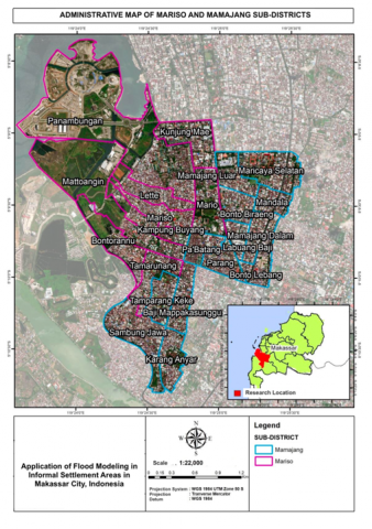
The research area consists of Mamajang District and Mariso District. Mariso District has an area of 1.82 km2 and Mamajang District has an area of 2.25 km2. The total area of the research area is 4.07 km2 (Table 1). The following is the area of each village in the research area. The following is the delineation of the research area illustrated in Figure 1.
Table 1. Area of villages in Mariso and Mamajang Districts
|
Neighborhoods |
Area (kilometer square) |
Percentage Area (%) |
|
Mariso District |
||
|
Pontorannu |
0.18 |
4.42 |
|
Tamarunang |
0.12 |
2.95 |
|
Mattoangin |
0.18 |
4.42 |
|
Kampung Buyang |
0.16 |
3.93 |
|
Mariso |
0.18 |
4.42 |
|
Lighten |
0.15 |
3.69 |
|
Mario |
0.28 |
6.88 |
|
Panambungan |
0.31 |
7.62 |
|
Kunjung Mae |
0.26 |
6.39 |
|
Mamajang District |
||
|
Paste Keke |
0.06 |
|
|
Continue Java |
0.3 |
1.47 |
|
3 New Coral |
0.2 |
7.37 |
|
Mappakasunggu Wedge |
0.15 |
4.91 |
|
Pa'batang |
0.11 |
3.69 |
|
Parang |
0.09 |
2.70 |
|
Bonto Lebang |
0.12 |
2.21 |
|
Mamajang Dalam |
0.19 |
2.95 |
|
Labuang Baji |
0.11 |
4.67 |
|
Bontobiraeng |
0.62 |
2.70 |
|
Mandala |
0.08 |
15.23 |
|
South Maricaya |
0.09 |
1.97 |
|
Outer Maricaya |
0.13 |
2.21 |
|
Total |
4.07 |
100 |
Source: Makassar City Central Statistics Agency, 2023 [5]
Figure 1. Research delineation map
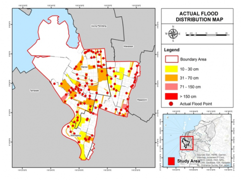
The actual distribution of floods is the flood condition that has occurred in previous years in the research area, namely Mariso and Mamajang Districts. This data is used to determine the distribution of flood points and areas, and it is also a benchmark for the validation of flood events that will be modeled in the formulation of the second problem. This data was obtained based on the results of interviews with local communities and stakeholders, namely village heads and employees who know the flood conditions in each sub-district in Mariso and Mamajang Districts. Then the non-spatial data is processed into spatial data using spatial analysis.
Based on interview data, 126 flood areas and flood points were produced spread across 22 villages in Mariso and Mamajang Districts. The distribution of floods is classified into four types of water depths, namely 10-30 cm, 31-70 cm, 71-150 cm, and > 150 cm. In addition to this classification, flood inundation times are also classified into three types, namely < 12 hours, 12-24 hours, and > 24 hours. In the results of flood data obtained, almost all villages in Mariso and Mamajang Districts have been affected by flooding in the past few years, especially in 2022 and 2021. The flood incident had an impact on community activities and the environment, namely the suspension of transportation access, buying and selling interactions, power outages, and evacuation of affected communities in a few days. The distribution of floods from the results of the interviews can be seen in Figure 2.
Figure 2. Map of the historical distribution of floods in the study area
In Figure 2, all villages in Mariso and Mamajang Districts were affected by flooding with several areas and flood points at these locations. The highest height of the puddle is in the outer Mamajang Village with a puddle height of 200 cm with a puddle duration of < 12 hours. Meanwhile, the lowest waterlogging height was in Labuang Baji and Tamparang Keke Villages with a waterlogging height of 10 cm and a duration of < 12 hours. In addition, waterlogging with a depth of 10 to 30 cm was reported in fourteen villages across two sub-districts. Then puddles at a height of 31-70 cm are in 12 villages. Meanwhile, the height of the puddle of 71-150 cm was found in six villages in two research districts. The difference in the height of waterlogging and the length of inundation can be influenced by the existing conditions of the affected area, such as the condition of the decrease in rainfall levels as well as the topography of the area, land cover, drainage, and roads.
Informal settlement areas are not only known based on local government administrative regulations but can also be identified through remote sensing of satellite imagery and validated based on field surveys on the physical characteristics of local settlement areas using standard parameters and morphological typologies of informal settlement areas where this area will be analyzed in an overlay manner with flood modeling results to see the spatial impact of flooding on residential areas slums in Mariso and Mamajang Districts. The standard parameters that can be identified through the image are as follows:
The spatial analysis to identify informal residential areas can also be identified through eight typologies of informal areas, namely, types in the form of areas (districts), being on the waterfront, slopes (escarpment), limited use land (easement), sidewalks, and relationships with the surrounding area (adherences), the back of the area (backstage), and the fence-shaped type (enclosure).
Based on the typology of informal settlement areas, it was identified that in the research area, there are many informal settlement areas spread across both Mariso and Mamajang Districts. The identified typology tends to be informal settlements growing at the back of formal buildings and spreading that follows the surrounding settlements in each village in the study area, while a few settlements are built on the water's edge along the canal in Lette, Mariso, Junction Jawa and Bontorannu Villages. The morphological shape of the informal settlement area can be seen in the mapping photo in Figure 3.
Figure 3. Photomapping of informal settlements in the research area
2.1 Factors of flooding
According to NOAA National Severe Storms Laboratory, flooding is the overflow of water into the land that is usually dry. Flooding can occur during heavy rains, when ocean waves come to shore, when snow melts quickly, and when dams or embankments break. Flooding can occur within minutes or over a long period of time, and can last days, weeks, or even longer.
Based on the study of Sudirman et al. [6], several factors causing flooding were explained, including:
2.2 Rainfall intensity distribution pattern
Gustoro [7] defined the rain distribution pattern as a rain distribution pattern where rain recording is usually carried out at a certain time interval, which is generally carried out in units of daily, hourly, or minute time. In order for the distribution of rain during the occurrence of rain to be known, it is better to record it with short time intervals.
Suroso (as cited in the study of Gustoro [7]) explained that rain intensity is the height of rainfall that occurs during the period when the water is concentrated, in units of mm/hour. The high intensity of rainfall is very important in the calculation of planned flood discharge based on the rational method of duration, namely the duration of a rain event.
2.3 Informal settlement areas
Informal settlements refer to residential areas that do not comply with and meet the requirements of the city authorities. These residential areas are informal and are usually located on land that is not intended for housing. The growth of these settlements is due to urbanization that is taking place faster than the government's ability to provide adequate land, infrastructure, and housing [9].
According to Western Cape Government [9], informal settlements have several distinctive features, including inadequate infrastructure, inappropriate environment, uncontrolled population density, poor quality of health, inadequate housing, poor access to education, health, and employment opportunities, and ineffective government and management. Therefore, these informal residential areas are at high risk of health problems, crime, and fires.
Informal settlements emerged as a result of a number of factors [9], including population growth and migration to cities, difficulty in accessing affordable housing for the urban poor, suboptimal governance (especially in urban land policies, planning, and management that have the potential to lead to land disputes), economic vulnerability and low-wage jobs, discrimination against marginalized groups, and relocation due to natural disasters, conflicts, and climate change.
In identifying areas that are included in informal settlement areas, there are several distinctive characteristics of these informal settlements. In determining informal settlement areas, research has provided a number of characteristics that can be identified through observation of satellite images. Some of these characteristics include the size of the building, the type of roofing material, the availability of roads, the presence of irregular roads, the lack of open space, the density or density of the building, and irregular settlement patterns. According to Alzamil [10], the typical characteristics of informal settlements include the size or area of the building, poor physical condition of the building, lack of facilities in the building such as toilets and kitchens, lack of children's play areas, poor access to clean water, inadequate wastewater disposal systems, inadequate waste management, and limited availability of green open spaces. Meanwhile, Msimang [11] highlighted characteristics such as the lack of waste management infrastructure, accessibility, toilet facilities, adequate sanitation, availability of clean water, and poor drainage systems in informal settlements.
2.4 Identification of informal settlement areas
Dovey and King [12] described various indicators that can be used to identify informal settlement areas through mapping using typology. Some of them are:
2.5 National Digital Elevation Model (DEMNAS)
Digital Elevation Model (DEM) data nationally is published by BIG and is known as DEMNAS (National DEM). DEMNAS is the result of the integration of several altitude data sources, including IFSAR data (5 m resolution), TERRASAR-X (5 m resolution), and ALOS PALSAR (11.25 m). Using these different types of data, DEMNAS has a spatial resolution of 0.27 arc-seconds.
The assimilation process in DEMNAS data was carried out using GMT-surface with a tension value of 0.32, referring to the research of Hell and Jakobsson (cited by Iswari and Anggraini [13]). The datum or vertical reference used in DEMNAS is the 2008 Earth Gravitational Model. This integrated data is also enriched with mass points through the assimilation process. Mass points are points that store three-dimensional coordinate information, namely x, y, and z on the earth's surface [13].
Thus, DEMNAS provides a digital representation of the earth's surface elevation nationally, with a high level of resolution and vertical consistency referenced in the 2008 Earth Gravitational Model. This data has many applications in various fields, including modeling topography, hydrology, slope analysis, and accurate mapping [13].
2.6 Land cover
According to the SNI 7645:2010 standard [14], land cover is defined as biophysical cover visible on the earth's surface, which comes from the results of human arrangements, activities, and treatment of certain types of land cover for production, alteration, or maintenance activities on the land cover. The land cover class consists of two main parts, namely vegetated areas and non-vegetated areas. Vegetated areas are divided into three types, namely agricultural areas and non-agricultural areas. Meanwhile, non-vegetated areas are divided into three types, namely built land, unbuilt land, and waters.
Land use change refers to the transformation of an area that previously had water catchment characteristics into a built-up area. This change generally occurs because most of the water catchment area is developed into a location for urban development, industry, economic activities, and settlements. An increase in the number of people in need of shelter is a major factor that reduces the extent of water catchment areas, which in turn leads to increased surface flow and flood risk.
2.7 Coefficient manning's rudeness
Chow (as cited by Sanusi and Pratiwi [15]) explained that one of the methods for calculating water flow discharge is the Manning method, which considers the environmental conditions around the channel and the components of the channel itself. The magnitude of the flow discharge in the channel is affected by the level of roughness of the channel base. The effect of roughness on the channel is expressed by a value called Manning's roughness coefficient. Factors that affect the value of the Manning roughness coefficient include the materials that make up the wet surface of the channel, the physical properties of the soil, the irregularity of the channel, the vegetation growing in the channel, and the process of sedimentation and erosion in the channel. If the channel is composed of materials such as gravel and skeleton, then the N Manning value is usually high, especially when the water level in the channel is high or low.
According to the SNI 2830:2008 standard [16], Manning's roughness coefficient is divided into three main categories, namely large rivers, flood banks, and small rivers. Small rivers themselves are divided into two types, namely rivers that flow in the lowlands and rivers that flow in the mountains. Meanwhile, large rivers have only one type, which is rivers that flow in lowlands. In addition, bank floods also have four types, namely banks that are used as pastures without shrubs, banks that are used as moors, banks that are overgrown with shrubs, and banks that have trees growing around them.
This Manning method is used to estimate the discharge of water flow in a channel by considering the physical characteristics of the channel and the surrounding environmental conditions. By taking into account the factors that affect Manning's roughness coefficient, this method aids in the planning and calculation of hydrology related to the flow of water in a channel.
2.8 Efficient runoff
Hadiyaturrohmi [17] explained the definition of runoff coefficient (C) is a parameter used to measure the proportion of rainwater that flows to the surface and cannot be absorbed by soil or infiltration. The runoff coefficient provides a comparison between the volume of surface runoff and the volume of rainfall that falls in an area.
In the context of hydrology, when rain falls in an area, part of the water will be absorbed by the soil (infiltration) and part of it will flow on the surface (runoff). The runoff coefficient is used to determine how much percentage of rainwater is surface runoff compared to the total volume of rainfall that falls.
The value of the runoff coefficient can vary depending on various factors, including soil characteristics, land cover, topography, rainfall, and the hydrological conditions of the region. Accurate and representative determination of runoff coefficient values is an important part of hydrological analysis, water system planning, and water resource management.
According to the SNI standard 03-2415-1991 Rev.2004 [18], the runoff coefficient (C) is divided into nine different categories. These categories include commercial areas, residential areas, industrial areas, fields, railway yards, uncultivated land, roads, grassy yards, and grassy yards of solid sand soil.
Each category has a different runoff coefficient value, which reflects the specific hydrological characteristics of each type of area. The runoff coefficient value is used to calculate or estimate the amount of surface runoff produced by rainwater in each type of area.
2.9 Geographic information system (GIS)
Esri UK as a company engaged in the application of geographic information defines a geographic information system (GIS) as a system that creates, manages, analyzes, and maps all types of data. GIS connects data to maps, integrating location data with all kinds of descriptive information. This provides a foundation for mapping and analysis used in science and almost every industry. GIS helps users understand patterns, relationships, and geographic contexts. The benefits include improved communication and efficiency as well as better management and decision-making.
Sugandi et al. [19] explained that GIS is a system designed to work with data that is spatially referenced or geographically coordinated. Anon (as cited by Sugandi et al. [19]) argued that GIS is an information system technology that can combine graphic data (spatial) with text data (attributes) of geographically connected objects on Earth (georeference). GIS can also combine data, organize data, and conduct data analysis that produces outputs that can be used as a reference in decision-making on problems related to geography.
2.10 Flood modeling software
Quoting from Goodarzi and Eslamian [4], flood modeling software or flood modeling applications are used to demonstrate the application's ability to forecast and forecast floods and river flows, its use in watersheds, and emphasis on its use on a larger scale than river flows for flood modeling management.
2.11 HEC-RAS software
The HEC-RAS software was developed by the Hydrologic Engineering Center (HEC) which is part of the U.S. Army Corps of Engineers. The software is designed to model open channel flows and other channels using one-dimensional flow modeling, under both permanent and impermanent flow conditions (steady and unsteady flow models) [4].
HEC-RAS can be used in the study of the spatial impact of floods on informal settlements in Mariso and Mamajang Districts, to simulate flood models in one-dimensional and two-dimensional visualizations. US Army Corps of Engineers [20], as a software developer HEC-RAS, provides information Use feature-feature to simulate as follows:
2.12 Model validity
Marfai and King [21] explained that the validation of the model carried out on flood modeling is a testing stage in calculating the accuracy level of the model. The accuracy value is an accurate parameter in a model, the accuracy value is obtained by using the confusion matrix method, which is to compare valid values and errors to get the percentage of model accuracy in this context can be compared based on the spatial of flood modeling which is compared with the spatial of the actual flood that has occurred. This validation method has been carried out by Marfai and King [21], by combining a 100-year river flood prediction model map obtained from JICA in 1993 with a tidal flood map obtained from the Works Office Semarang General in 2001, then from the results obtained spatial slices that were flood-validated so that the model accuracy test method on the confusion matrix tabulation could be carried out.
This research is a type of descriptive research with a quantitative qualitative approach presented in the form of descriptions, images, tables, and maps. The analysis used was quantitative descriptive analysis, qualitative analysis, spatial analysis and literature synthesis.
The types of data needed are primary data and secondary data. The data collection techniques used are Literature Review, Observation, Documentation, and Interview. The analysis techniques used are Qualitative Descriptive, Quantitative, Spatial Analysis, and Flood Modeling Analysis.
3.1 Research location
The location of this research is Mariso District and Mamajang District, Makassar City, South Sulawesi. The map of the research location can be seen in Figure 4 below.
Figure 4. Research location
3.2 Data collection technique
This research employs both primary and secondary data collection methods to support the flood modeling analysis in informal settlement areas within Mariso and Mamajang Sub-districts, Makassar City. The integration of spatial and non-spatial data is essential to simulate flood conditions accurately and to understand their impact on vulnerable urban communities.
a. Primary Data Collection
Primary data were obtained through direct field observations and GPS-based ground checking. The field survey aimed to validate the actual conditions of informal settlements, land cover types, and flood-prone areas. Ground truthing was conducted to verify the accuracy of remote sensing data and to assess the real extent of flood impact. Interviews with local residents and community leaders were also carried out to gather qualitative insights about historical flood events, drainage conditions, and community responses.
b. Secondary Data Collection
Secondary data were collected from relevant government agencies and official institutions. Rainfall data were obtained from the Meteorology, Climatology, and Geophysics Agency (BMKG) through the Tamalanrea Climatology Station, which is the closest station to the study area. Tidal data were sourced from the Makassar Paotere Port Authority to capture sea-level conditions that contribute to coastal flooding. National Digital Elevation Model (DEMNAS) data were accessed via the BIG, while land use and administrative boundary maps were collected from the Makassar City Spatial Planning Agency (Dinas Tata Ruang Kota Makassar). Quality control procedures were applied to ensure the reliability of all datasets, including completeness checks, removal of anomalies, and consistency evaluations with historical records. These data were chosen for their relevance, accuracy, and representativeness in capturing the hydrological and spatial characteristics of the study area.
3.3 Flood modeling
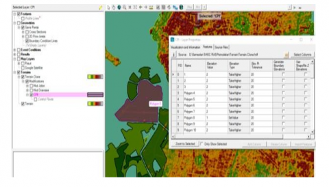
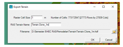
Flood modeling is a method used to model flood simulations in the research area to identify the spatial impact of floods. The flood modeling method in the HEC-RAS software has four sub-variables that are used systematically and gradually to simulate floods, the first stage is to modify the land (Figure 5), the second is to make a two-dimensional water flow geometry (Figure 6), the third is to enter the spatial data of the land cover (Figure 7), and the fourth is to run an unstable flow simulation program (Figure 8 and Figure 9). Then the results will be identified and reprocessed to compare the spatial impact of flooding on informal settlement areas. The first stage is to make modifications to the DEM or terrain. This modification is carried out to change the resolution and surface of the terrain that is not detailed to very detailed so that it can improve the accuracy of flood modeling on an urban scale and is also used to change the terrain area just like the current surface conditions. The stages of modification are as follows:
Figure 5. Modification of reclaimed land
Figure 6. Waterflow geometry modification
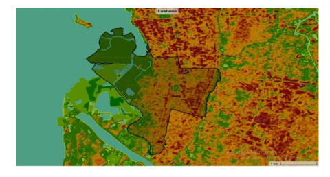
Figure 7. Land cover modification
Figure 8. Terrain modification results
Figure 9. Terrain modification results
The next sub-variable of flood modeling is to create a 2-dimensional water flow geometry. This stage aims to limit the area of the rainfall area and provide the direction of the tidal flow of the sea so that the 2-dimensional water flow is divided into 2 indicators, namely perimeter (regional rainfall) and boundary condition lines (tidal and tidal seawater). It was carried out by digitizing the Thiessen rainfall area and digitizing the coast or coastline in the research area, after which on the rainfall perimeter indicator, the number of mesh cells was calculated which aimed to detect sub-variables, namely terrain and land cover.
(1) Perimeter (Rainfall area). The 2-dimensional water flow perimeter has 3 parts, namely the perimeter of Paotere station, Region IV station and Barombong station. The perimeter will be computed at each cell point to detect rainfall analysis that will be programmed, in addition to cell point computing aims to detect errors in the 2-dimensional water flow perimeter. The size of the cell used is 10 m which is considered large area of the research area. The following is a view of the perimeter of the rainfall area and cell computing in Figure 10.
(2) Boundary condition lines. The boundary condition line is an indicator used to include the sub-variable of the tide of sea water, because in existing flood conditions it is also affected by the tides. At this stage, the digitization of boundary condition lines along the coast or coastline of the research area will be carried out, where the indicator will be included in the data on the height of the tide of sea water in the analysis of impermanent flows (Figure 11).
Figure 10. Area perimeter and cell computing
Figure 11. Boundary condition lines
4.1 Flood modeling results
The results of flood modeling are the results of spatial analysis in HEC-RAS software which has gone through several work processes starting from the processing of non-spatial data, namely the calculation and distribution of the distribution of rainfall intensity levels and tides of sea water, then continued with the process of adjusting existing conditions on spatial data such as updating the terrain model, entering absorption and runoff values rainwater and adjust the 2D flow area limits in accordance with the scope of the research area.
Flood modeling produces several flood simulation models in the research area, the modeling is a scenario based on variable factors, a simulation of the rate of altitude based on flood time, a simulation of flood water flow, and the validation of flood models against actual floods. Some of these models were carried out to identify how much flood impact was generated from flood modeling analysis using HEC-RAS software so that it could be associated with spatial impacts on informal settlements in the research area. The results of the flood modeling, then a spatial analysis was carried out using ArcGIS software to obtain information related to the influence and impact of the flood spatially.
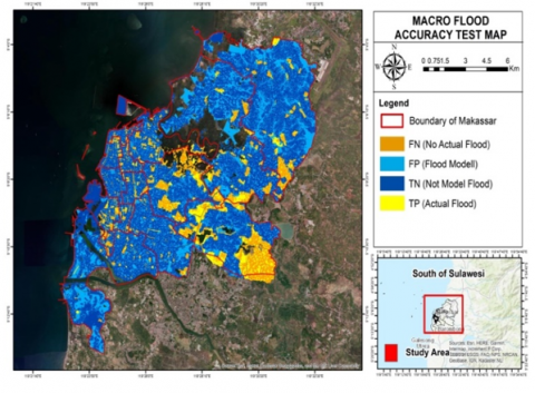
4.2 Macro-scale flood model scenario
The macro-scale flood model scenario is to model a flood on a scale of one area of Makassar City, this method is used to determine the relationship between the impact of the flood model between the research area and the adjacent area. At this stage, several scenarios were carried out, namely by testing 30 scenarios, where the scenario was a HEC-RAS simulation experiment carried out by varying rainfall based on data from five rainfall monitoring stations, the average rainfall of Makassar City, and flood-causing factors, resulting in a total of 30 different simulation models. Then, the modeling results are evaluated to measure the level of accuracy using a confusion matrix, with the aim of identifying and selecting the simulation model that has the highest level of accuracy. The simulation results can be shown in Table 2 and Figure 12.
Table 2. Simulation results and accuracy values of each scenario
|
Scenario |
Rainfall |
Flood Height (meter) |
Flood Area (hectare) |
Accuracy (%) |
|
I |
Average Makassar City |
4.97 |
7,243 |
52.75 |
|
IS Barombong |
4.83 |
5,787 |
59.21 |
|
|
STA Paotere |
5.49 |
7,146 |
53.13 |
|
|
STA Region IV |
5.67 |
7,924 |
50.02 |
|
|
STA Biring Romang |
4.40 |
5,879 |
58.77 |
|
|
STA Sultan Hasanuddin |
5.62 |
9,990 |
51.90 |
|
|
Average Makassar City |
4.96 |
7,167 |
53.17 |
|
|
II |
IS Barombong |
4.68 |
5,642 |
60.02 |
|
STA Paotere |
5.52 |
7,058 |
53.51 |
|
|
STA Region IV |
5.69 |
7,865 |
50.01 |
|
|
STA Biring Romang |
4.40 |
5,736 |
59.60 |
|
|
STA Sultan Hasanuddin |
5.62 |
9,337 |
50.41 |
|
|
III |
Average Makassar City |
5.01 |
7,487 |
51.24 |
|
IS Barombong |
4.33 |
6,347 |
55.78 |
|
|
STA Paotere |
5.00 |
7,390 |
51.62 |
|
|
Regional STA IV |
5.25 |
8,131 |
48.75 |
|
|
STA Biring Romang |
4.44 |
6,418 |
55.46 |
|
|
STA Sultan Hasanuddin |
5.72 |
9,721 |
48.06 |
|
|
IV |
Average Makassar City |
5.02 |
7,214 |
52.87 |
|
IS Barombong |
4.41 |
5,774 |
59.25 |
|
|
STA Paotere |
5.01 |
7,117 |
53.23 |
|
|
Regional STA IV |
5.24 |
7,917 |
50.06 |
|
|
STA Biring Romang |
4.36 |
5,879 |
58.76 |
|
|
STA Sultan Hasanuddin |
5.89 |
9,337 |
52.47 |
|
|
V |
Average Makassar City |
5.01 |
7,443 |
51.48 |
|
IS Barombong |
4.79 |
6,292 |
56.10 |
|
|
STA Paotere |
5.61 |
7,340 |
51.86 |
|
|
Regional STA IV |
5.24 |
8,096 |
48.91 |
|
|
STA Biring Romang |
4.34 |
6,371 |
55.79 |
|
|
STA Sultan Hasanuddin |
5.85 |
7,600 |
49.93 |
Figure 12. Makassar City flood model accuracy test map
4.3 Scenarios based on micro-scale flood factors
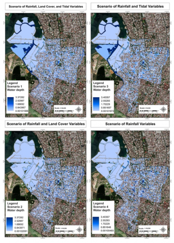
Flood modeling scenarios are designs carried out on a micro-specific basis in the research area to determine the differences between the uses of each sub-variable factor as a comparison of the effects of land cover use, tides and rivers on changes in flood simulation distribution patterns. Flood modeling is designed in the following five scenarios:
Figure 13. Comparison of scenario maps
Based on the comparison of scenario maps in Figure 13, differences between the four scenarios can be identified. The result of the interpretation of the scenario map on each variable factor is that it only has a water level that is not much different. Then it was identified that the first scenario (I) using land cover and sea tide factors there were flood water level classifications of 84 cm, 168 cm, 252 cm and 337 cm which had similarities in the third scenario (III) which used the influence of tidal factors and without land cover factors. However, the difference between the two scenarios lies in the water level that occurs in the Mattoangin field, the water level in the Mattoangin field area in scenario III was identified as an expansion of the water level in the water level classification of 300 cm, this is influenced by the absence of land cover variable factors in scenario III.
Meanwhile, in the fourth scenario (IV) with the flood model without using any flood factors, a slight increase in the water level on the coast in the research area was identified, namely with the flood water level classification level of 85 cm, 170 cm, 255 cm, and 340 cm. Meanwhile, in the second scenario (II) with the flood model only using the land cover factor, it was identified that there was a decrease in water level in the coastal area, this was caused by The influence of flood driving factors from the factors that cause sea tides.
The interpretation in all four scenarios is that each variable factor has a different influence. Because the influence was chosen one scenario that has factors that are close to the actual natural conditions that can affect the occurrence of floods, the chosen scenario is scenario I because it has factors that cause flooding in accordance with the real conditions presented by Sudirman et al. [6].
4.4 Simulation of water depth rate based on flood time
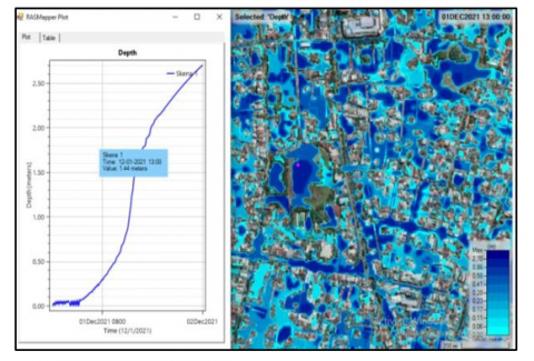
The model in the simulation of the water depth rate based on the flood time is divided into three simulation models, namely the flood simulation at the 12th hour, the flood simulation at the 24th hour, and the combined maximum flood simulation of the entire flood hour. The results of this simulation will be identified related to the area, depth rate, and highest point of flooding in the simulation model.
Based on the interpretation of the map, it can be seen that the distribution of stagnant water in this simulation model covers the entire research area. The analysis of the water level at this hour resulted in five different classifications, namely 0.33 – 0.74 m, 0.75 – 1.25 m, 1.26 – 1.87 m, and 1.88 – 3.37 m.
The spatial simulation of the flood at the 12th hour can be seen visually in Figure 14. Meanwhile, in looking at the level of water level at the 12th hour at the location point of the Mattoangin field, it was identified that at 12.00 on December 1, 2021, the flood water level was recorded at 1.44 meters. This is shown in Figure 15 (Table 3).
Figure 14. Flood simulation map at the 12th hour in scenario 1
Figure 15. Highest flood in the 12th hour in scenario 1
Table 3. Depth and area of flood pad at 12th hours
|
Water Level 12th Hour (meter) |
Flood Area (kilometer square) |
|
0.33 - 0.74 |
0.3862 |
|
0.75 - 1.25 |
0.0236 |
|
1.26 - 1.87 |
0.0043 |
|
1.88 - 3.37 |
0.0003 |
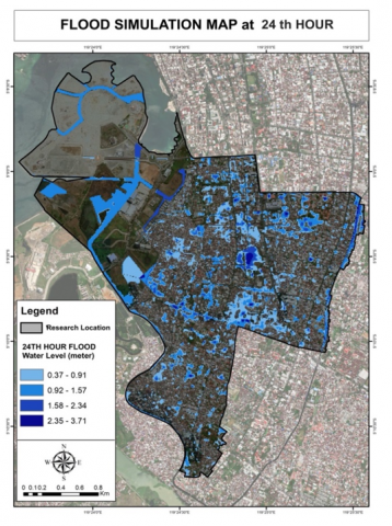
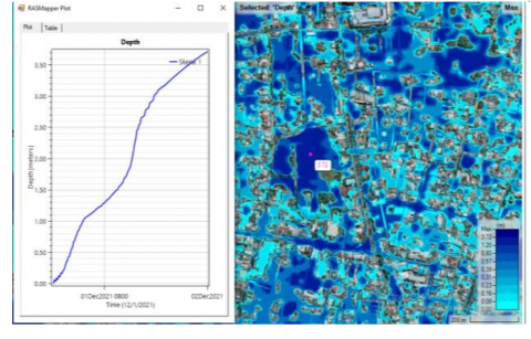
The results of the flood simulation at the 24th hour are shown in Figure 16 that the distribution of the flooded water model is different from the 12th hour, where at the 24th hour it is seen that some number of water level classifications in the coastal area in Mattoangin Village are missing. The water level at the 24th hour has four classifications of water level, namely 0.37 - 0.91 m, 0.92 - 1.57 m, 1.58 - 2.34 m, and 2.35 - 3.71 m. For this, it was identified that there was an increase in the amount of water at the 24th hour, so the classification of water level values also increased. Looking at the graph table in Figure 17, the highest flood point height was identified in the Mattoangin field with a flood water level of 3.71 meters. Graphically, the water level in the Mattoangin field continues to increase every hour.
Figure 16. Flood simulation map at the 24th hour in scenario 1
Figure 17. Highest flood in the 24th hour in scenario 1
The flood area recorded in Table 4 based on the simulation map of the 24th hour, that the smallest flood area was found at the water level of 2.35 - 3.71 m with a flood area of 0.61 km2. Meanwhile, the largest flood area is at a water level of 0.37 - 0.91 m with an area of 1,773 km2. When compared to the flood model simulation at the 12th hour, the increase at the 24th hour tends to increase and has the greatest flood impact at the water level of 0.37 - 0.91 m, then 0.978 km2 at the water level of 0.92 - 1.57 m, and 0.489 km2 at the water level of 1.58 - 2.34 m. This is influenced by the rain that continues to occur, which increases the water discharge in areas on the surface which tends to be lower.
Table 4. Depth and area of the flood pad at the 24th hour
|
Water Level 24th Hour (m) |
Flood Area (km2) |
|
0.37 - 0.91 |
1.773 |
|
0.92 - 1.57 |
0.978 |
|
1.58 - 2.34 |
0.489 |
|
2.35 - 3.71 |
0.61 |
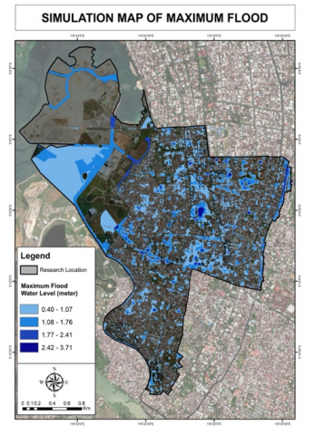
The depth and area of the flood area is maximum. The results of the maximum flood simulation are the maximum flood collection at each place from all hours. The maximum flood map is shown in Figure 18 that the water level at the maximum has four height classifications, namely 0.40 - 1.07 m, 1.08 - 1.76 m, 1.77 - 2.41 m, and 2.42 - 3.71 m. Spatially, the maximum distribution of the flood model was identified and the flood spread throughout the study area. The graph generated from the simulation of the maximum flood model has the same rate of water level in each hour. However, in terms of distribution pattern, because the maximum flood simulation combines the maximum water level in each hour, the distribution of flood water levels is more than that of the flood simulation model at the 12th and 24th hours. A graph of the rate of increase in water level can be seen in Figure 19.
Figure 18. Maximum flood simulation in scenario 1
Figure 19. Maximum flood in scenario 1
4.5 Flood water flow simulation based on inundation time
The flood water flow simulation model is an illustration of water flow that is influenced by inhibiting and driving factors by different terrain conditions and driven by the tidal flow of seawater. The movement of flood water flow will be seen in the flood model simulation at both flood hours, namely at the 12th hour and at the 24th hour. This is due to the height and low of the ground surface (terrain) that has been modified from the spatial data indicators of drainage and roads so that it can be an inhibiting factor from various water flows.
In the flood water flow simulation, it is identified through images and layers of water flow results which aims to see the influence of these inhibiting and driving factors. In addition, it can also increase the accuracy of flood modeling in the research area, namely Mariso and Mamajang Districts.
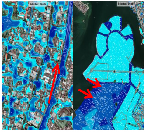
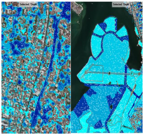
Figure 20. (Left) the flow of water around the canal, and (right) the flow of coastal water at the 12th hour
Figure 21. (Left) water flow around the canal, and (right) coastal water flow at the 24th hour
4.6 Flood water flow simulation based on inundation time
The flood modeling that has been analyzed is based on non-spatial data, namely rainfall, tides, coefficients, roughness of manning and runoff, as well as raster spatial data, DEM, google satellite imagery, as well as vector data such as shapefiles of flood points and actual flood areas will be components to validate the level of compatibility of flood modeling with actual floods using the layer overlay method and conduct an accuracy test through the data comparison method on the Confusion Matrix to analyze the combined pixel values between the actual flood and the flood model.
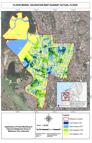
The analysis is shown in Figure 22 by displaying the mapping results of the intersect layer overlay. The map clearly depicts the distribution of the areas described earlier. Through this spatial analysis, it can be more in-depth information about the extent to which flood modeling can represent a fit and test the ability of flood models in potentially affected areas in actual flood situations.
Figure 22. Map of flood model validation against actual flooding
The validation stage of flood modeling for location flooding aims to test how accurate the results of flood modeling analysis on location flooding are. Departing from this, the confusion matrix method is carried out to determine the level of accuracy of flood modeling. The classification of values in the confusion matrix obtained from the number of raster pixels resulting from the overlay of the flood model and the actual flood is shown in the following Table 5.
Table 5. Validity test of the flood model
|
Current |
|||
|
Classification |
Flood |
No Flood |
Ground Truth |
|
Flood |
(TP) 171,317 |
(FP) 768.577 |
939.894 |
|
No Flood |
(FN) 339.312 |
(TN) 2,299,130 |
2.638.442 |
|
Total |
510.629 |
3.067.707 |
3.578.336 |
|
Accuracy |
69.03% |
||
Based on Table 5, it is known the number of pixels resulting from layer overlays to perform matrix calculations. It is known that true positive (TP) is the overlay of the actual flood screen and the flood model has a value of 171,317 pixels, false positive (FP) is the overlay of the actual non-flood screen and the non-flood model has a value of 168,577 pixels, then false negative (FN) is the overlay of the screen of the unflooded and actual flooded models have a value of 339,312 pixels, while true negative (TN) is the overlay of the actual unflooded screen and the unflooded model has 2,299,130 pixels. The number of pixels obtained is then tested for validation calculation with the formula for determining the percentage of model accuracy, namely:
Accuracy $=\frac{171.317+2.299 .130}{3.578 .336} \times 100 \%=69.03 \%$
Thus, the results of the calculation resulted in a total accuracy percentage of 69.03%. Based on research conducted by Talampas and Tarepe [22], the percentage of accuracy of flood models at the level of 72% has a fairly strong accuracy capability, so from this statement, the results in flood modeling can be said to be close to the accuracy category which is quite strong because it has an accuracy value of 69.03%. In addition, it is also mentioned that if the accuracy level is close to 100%, the modeling results can be used for further analysis. However, on the other hand, after identification through flood data, it was found that what caused the model results not to reach 100% accuracy was due to the lack of complete actual flood data that spread throughout the research area, so there were still many gaps to match the model flood.
4.7 Distribution of spatial impact of floods in informal settlements
Modeling the spatial impact of floods on informal settlements is the third problem formulation in this study which aims to identify the spatial impact of floods on informal settlement areas. Spatial impact floods have three problem indicators, namely the area of the affected area, the depth of water and the percentage of flood-affected areas. The spatial impact of flooding on informal areas is shown in Figure 23.
Based on Figure 23, it is identified that out of 71 areas of the number of informal settlement areas identified, there are only 60 areas of the total number of informal settlement areas affected by floods. The villages affected by the flood are based on informal settlement areas of the 22 villages, there are only 19 affected villages, namely Kunjung Mae, Panambungan, Lette, Mariso, Kampung Buyang, Mattoangin, Bontorannu, Mario, Tamarunang, South Maricaya, Bonto Biraeng, Mandala, Bonto Lebang, Parang, Pa'Batang, Baji Mappakasunggu, Tamparang Keke, Connect Jawa, and Karang Anyar. The flood water level spread in informal residential areas is quite diverse, based on the water level classification in each area is detailed at the water level of 10-30 cm, 31-70 cm, 71-150 cm, 200 cm, and 300 cm.
The classification of highest water level in informal settlement areas that were identified as having a water height of 71-150 cm was in Mattoangin Village in the informal settlement area with the typology of the built area along the land boundary wall, then with the water height of 300 cm in the area built by the edge water bodies or canals are located in the informal settlement area in Mattoangin Village. The flood area spread in informal settlement areas based on the results of spatial analysis using the intersect layer overlay method, it was identified that the largest flood impact area was in Parang Village with a flood impact area of 0.88 ha at a water level of 10-30 cm. Then the second largest flood area is in the informal settlement area in Mariso Village with a flood impact area of 0.40 ha at a water level of 31-70 cm. Meanwhile, in some informal settlement areas affected by floods with water levels as high as 200 cm, but rather than that, water levels with a height of 300 cm do not have a wide range of impacts but have flood water levels that tend to be very high.
Figure 23. Map of the spatial impact model of flooding in informal settlement areas in Mariso and Mamajang sub-districts
4.8 Illustration 1 dimension of the spatial impact model of flood
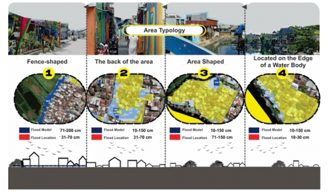
In Figure 24, the impact of the flood disaster is depicted in the form of a 1D front view of a slice of residential building pieces integrated with the height limit between the flood model and the actual flood height. This process helps provide a clearer visual picture of how floods impact informal settlements. Using this illustration, several different typologies of informal settlement areas can be identified, such as areas with a fence shape, the back of the area, an area with a certain pattern that shows, and areas located on the water's edge are illustrated to have a potential flood risk in each character of the settlement area.
Informal settlement areas have various typologies that affect the impact of flooding. The fence-shaped typology has minimal impact because the actual water level is lower than the flood model. In the typology of the back of the area, houses with low ground level can be affected flood. The typeface in the form of a spreading area has a limited impact thanks to good water flow facilities. In the typology of the edge of a water body, houses are rarely affected because the flow of canal water effectively reduces the impact of flooding, but houses on the canal are still at risk of being submerged.
Figure 24. The illustration of floods based on the typology of informal settlement areas
Based on the results of the analysis that has been carried out, the following conclusions can be obtained.
Based on the results and discussions that have been presented. This research has several suggestions or inputs to be carried out in the future, the suggestions are as follows:
[1] Mahardy, A.A. (2014). Analysis and mapping flood-prone areas in Makassar City are spatially based. Undergraduate Thesis, Hasanuddin University. University Repository Hasanuddin. http://repository.unhas.ac.id/handle/123456789/11965.
[2] Geospatial Information Agency. (2019). Ina-Geoportal Flood Disaster Data of Makassar City. https://tanahair.indonesia.go.id/portalweb/bencana/metadata_sulsel.html, accessed on May 15, 2023.
[3] Makassar City Regional Regulation No. 4 of 2015 concerning Makassar City Regional Spatial Plan 2015-2034. https://jdihn.go.id/files/147/perdano.4thn2015.pdf, accessed on Apr. 25, 2023.
[4] Eslamian, S., Eslamian, F. (2022). Flood Handbook: Analysis and Modeling (1st ed.). CRC Press. https://doi.org/10.1201/9780429463938
[5] Central Statistics Agency of Makassar City. (2023). Makassar City in 2023 Figures.
[6] Sudirman, T.S., Barkey, R.A., Ali, M. (2017). Factors the affecting floods/inundation of city beach and its implications for waterfront areas. Seminar National Space #3: 141-157. https://www.scribd.com/document/614333139/Factors A ffecting-Flooding-Inundation-in-the-city-coast-and-its implications-Waterfront-FacingArea#, accessed on Mar. 24, 2023.
[7] Gustoro, D. (2018). Hourly rainfall distribution pattern analysis in progo watershed. Thesis Bachelor, Islamic University of Indonesia. Dura Space University Islam Indonesia. https://dspace.uii.ac.id/handle/123456789/11991.
[8] Erwanto, N.H., Yulianti, E., Surbakti, S. (2021). Planning of boezem and pumps in flood management in Pasuruan Regency, East Java. Journal Sondir, 5(2): 40-48. https://doi.org/10.36040/SONDIR.V5I2.4194
[9] Western Cape Government. (2013). Informal Settlements Handbook. Africa South: Wester Cape Government. https://www.westerncape.gov.za/generalpublication/informal-settlements-handbook, accessed on May 20, 2023.
[10] Alzamil, W.S. (2018). Evaluating urban status of informal settlements in Indonesia: A comparative analysis of three case studies in North Jakarta. Journal of Sustainable Development, 11(4): 148. https://doi.org/10.5539/jsdv11n4p148
[11] Msimang, Z. (2017). A study of the negative impacts of informal settlements on the environment. A case study of Jika Joe, Pietermaritzburg (Master of housing). School of Built Environment and Development Studies: University of KwaZulu-Natal, Howard College Campus. https://researchspace.ukzn.ac.za/handle/10413/16293.
[12] Dovey, K., King, R. (2011). Forms of informality: Morphology and visibility of informal settlements. Built Environment, 37(1): 11-19. https://doi.org/10.2148/benv.37.1.11
[13] Iswari, M.Y., Anggraini, K. (2018). DEMNAS: National elevation digital model for coastal applications. Oceana, 43(4). https://doi.org/10.14203/oseana.2018.vol.43no.4.2
[14] National Standardization Agency. (2010). Classification of land cover (SNI 7645:2010). https://www.big.go.id/assets/download/sni/SNI/15.%20SNI%2076452010%20Classification%20penutup%20lahan.pdf, accessed on Jul. 12, 2023.
[15] Sanusi, W., Pratiwi, V. (2020). Coefficient evaluation manning on the different basic types of channels. Cantilever, Journal of Engineering Research and Studies Civil.
[16] National Standardization Agency. (2008). Procedure for calculating river water level height by pias method based on manning formula (SNI 2830:2008). http://water.lecture.ub.ac.id/files/2012/05/15133_SNI-2830_2008_tata-how-tal-calculation-height-face-water-river-dg-cara-pias-dg-rumus-manning.pdf, accessed on Jul. 10, 2023.
[17] Hadiyaturrohmi, L. (2021). Analysis runoff coefficient (C) in the reak watershed, Bayan District, North Lombok Regency. Undergraduate Thesis, University They killed. Eprints Hasanuddin University. http://eprints.unram.ac.id/id/eprint/20796.
[18] National Standardization Agency. (2004). Procedure for calculating flood discharge (SNI 03-2415-1991 Revision 2004). https://id.scribd.com/document/523809518/SNI03-2415-1991-Rev-2004#, accessed on May 25, 2023.
[19] Sugandi, D., Somatri, L., Sugito, N. (2009). Information systems geographic (SIG) bandung: Geography education, Faculty of Social Sciences Education, University of Education Indonesia. http://file.upi.edu/Direktori/FPIPS/JUR._PEND._GEOGRAFI/195805261986031DEDE_SUGANDI/HAND_OUT_SIG.pdf, accessed on Mar. 4, 2023.
[20] US Army Corps of Engineers. (2023). HEC-RAS river analysis system creating land cover, manning’s N values, and % impervious layers. In US Army Corps of Engineers. US Army Corps of Engineers. https://rashms.com/wp- content/uploads/2021/06/HEC-RAS-2D-Mannual-Mannings-n.pdf, accessed on Apr. 20, 2023.
[21] Marfai, M.A., King, L. (2007). Monitoring land subsidence in Semarang Indonesia. Environmental Geology, 53(3): 651-659. https://doi.org/10.1007/s00254-007-0680-3
[22] Talampas, W.D., Tarepe, D.A. (2019). Delineation of flood-prone areas in data-scarce environment using linear binary classifiers. Mindanao Journal of Science and Technology, 17: 214-226. https://mjst.ustp.edu.ph/index.php/mjst/article/view/270, accessed on Mar. 24, 2023.