Hasdi Aimon![]() | Anggi Putri Kurniadi*
| Anggi Putri Kurniadi*![]() | Sri Ulfa Sentosa
| Sri Ulfa Sentosa![]() | Nurhayati Abd Rahman
| Nurhayati Abd Rahman![]()
© 2024 The authors. This article is published by IIETA and is licensed under the CC BY 4.0 license (http://creativecommons.org/licenses/by/4.0/).
OPEN ACCESS
This study aims to test the endogeneity among green growth, foreign debt, and aging population for Indonesia and Malaysia using a vector autoregression approach from 1975 to 2023. This study can provide important insights into how economic and demographic factors interact in the context of green growth and foreign debt, as well as offer more informed policy recommendations for both countries. Endogeneity analysis in this context will help design more effective and adaptive policies to address global and local economic dynamics toward achieving sustainable development goals. The key findings of this study indicate similar results in both countries, showing causality between the aging population and foreign debt. Furthermore, there is a one-way relationship where only green growth affects foreign debt. Additionally, there are divergent findings between the two countries: green growth and aging population do not influence each other in Indonesia, whereas in Malaysia, it is only aging population that affects green growth. Recommendations from this study suggest that both countries need to promote sustainable health for aging populations through the development of productive investments and risk management in the use of foreign debt.
aging population, foreign debt, green growth, vector autoregression
The issue of green growth (GG) is a critical indicator in assessing the performance and success of a country, which trend is closely related to the use of inputs to generate total output over a specific period [1]. The GG trend refers to the utilization of economic inputs to achieve high output within a particular period while considering the comprehensive environmental impacts [2, 3]. Various types of inputs as components of production factors used in economic activities include resources, which can be classified into capital resources and human resources [4]. In this regard, the increasingly widespread globalization does not negate a country's ability to obtain capital resources from abroad through foreign debt (FD) [5]. Additionally, human resources can refer to the population [6, 7].
Factors of production from capital resources, particularly those sourced from FD, refer to capital obtained through loans acquired from institutions or other countries. This can include international bank loans, international bonds, or credits from international financial institutions [8]. Funding from FD is utilized to enhance a country's production capacity, finance infrastructure projects, industrial development, or other investments aimed at fostering economic growth (EG) [9, 10]. However, the use of FD requires careful consideration regarding repayment risks, interest costs, and overall economic impact. Generally, these production factors play a crucial role in the global modern economy, where access to FD can accelerate a country's EG, but must also be managed prudently to avoid excessive dependence or uncontrolled financial risks [11, 12].
Meanwhile, factors of production from human resources, referring to the population, constitute the economically active portion of the population. The size and composition of the population significantly influence a country's production capacity [13, 14]. Countries with large and skilled populations typically generate more goods and services [15]. However, the focal issue concerning human resource factors of production is the aging population (AP), as it leads to a decline in the proportion of the population that is economically active. This can reduce the available workforce to meet production and service needs, thereby affecting EG potential [16]. Moreover, an AP does not contribute to a country's output growth, thus slowing its EG. Additionally, an AP aggregates economic burdens on a country because this elderly group requires more medical care compared to younger age groups.
Previous literature reviews have identified studies on this topic, but a significant gap necessitates further analysis. Existing studies tend to be conventional, overlooking the concepts of GG and neglecting endogeneity and comparative analysis. For instance, Lopreite and Mauro [17] analyzed emerging economies from 1990 to 2015, finding that FD had a significant negative impact on EG due to its non-productive application. Similarly, research by Kharusi and Ada [18] in Ukraine from 2006 to 2016 revealed that high FD coupled with macroeconomic instability hindered EG. Additionally, Shkolnyk and Koilo [19] studied the Economic Community of West African States from 1990 to 2016, highlighting FD as a capital source that could enhance healthcare expenditure, thereby impacting the AP. Meanwhile, N’Zue [20] conducted research in Croatia from 2004 to 2019, indicating that an unbalanced AP to productive age population ratio leads to reduced EG. These findings were reinforced by Buterin et al. [21], who found across countries that an increase in AP, combined with adequate human resource quality, enhances EG. Therefore, this research fills this gap by exploring the endogeneity between GG, FD, and AP towards achieving sustainable development (SD).
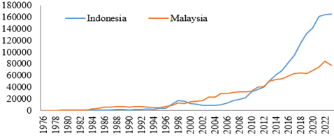
Figure 1. GG in percent [24]
Figure 2. FD in millions of USD dollars [24]
Figure 3. AP in percent of the total population [24]
SD represents a correction to the classical development model that solely focuses on EG and serves as an anticipation of development activities exceeding the carrying capacity of natural resources and the environment [22]. Furthermore, achieving SD also holds the potential to enhance environmental sustainability while ensuring future generations are not compromised due to the current economic system [23]. Moreover, GG, FD, and AP, upon scrutiny and analysis, can be interconnected in several ways. GG is believed to offer new investment opportunities that can help address economic challenges arising from AP through increased demand for environmentally friendly technologies and healthcare services. On the other hand, prudent management of FD can provide funding for GG investments and infrastructure to support AP. However, it is crucial to investigate that the relationship between GG, FD, and AP may vary from one country to another due to each country's unique economic context. Based on this explanation, GG, FD, and AP are part of macroeconomic indicators believed to have interdependencies in the context of SD in a country, particularly in Indonesia and Malaysia, which are classified as upper-middle-income countries in the Association of Southeast Asian Nations (ASEAN). These conditions are summarized in Figures 1-3.
Based on the information in Figures 1-3, the phenomenon observed is that GG in Indonesia tends to be higher compared to Malaysia during the observation period. However, the FD condition in Indonesia is larger than in Malaysia. Additionally, the AP trend in Malaysia shows a more significant increase compared to Indonesia. Ideally, high GG in Indonesia should help reduce dependence on foreign resources like FD to enhance economic self-reliance. However, Indonesia's FD is larger than Malaysia's, which contradicts previous literature findings. FD has the potential to become a heavy burden on the economy due to substantial annual interest and principal debt payments. This could potentially limit Indonesia's ability to allocate resources towards sustainable development, including GG and services needed by the AP. Based on these phenomena, the interdependencies between GG, FD, and AP in these two countries are not evident yet.
There are several challenges in achieving SD through GG, FD, and AP. One of the key challenges in achieving optimal GG is how to allocate factors of production efficiently and implement appropriate policies to stimulate sustainable GG. On the other hand, a challenge for FD is that interest and principal debt payments can consume a significant portion of a country's income, hindering the ability to invest in infrastructure and other public services [25-27]. Managing FD is a complex challenge for many countries, requiring wise policies to minimize associated risks [28, 29]. Meanwhile, the challenge for AP is placing additional pressure on pension systems and healthcare services, as governments must ensure that the AP group has sustainable strategies to address increasing needs, while also promoting greater economic participation from older individuals [30, 31].
In the context of SD, Indonesia and Malaysia exhibit unique characteristics and face different challenges. However, through comparative analysis, these countries can learn from each other to optimize efforts toward inclusive SD. Specifically, the interrelation of GG, FD, and AP presents crucial issues that are important to analyze, drawn from various studies to support the focus of this research. First, GG is part of development indicators focusing on SD by prioritizing environmental protection and committing to reducing negative impacts on ecosystems [32]. Implementation of GG involves investments in environmentally friendly technologies and practices, such as renewable energy, energy efficiency, sustainable transportation, and improved waste management [33]. Additionally, GG aims to enhance economic and social well-being while minimizing carbon emissions and other negative environmental impacts [34]. Second, FD refers to funds borrowed by a country from foreign creditors, which can be used to finance economic investments and development like infrastructure, education, and other public services [17]. However, excessive FD can burden a country's economy if not managed properly, due to required interest and principal repayments, with risks of default [35, 36]. Third, AP refers to the increase in the proportion of the elderly population within a population, which can impact the economy in various ways, including changes in the workforce structure, demand for healthcare and long-term care services, and disparities in consumption of goods and services by younger generations [37, 38].
There are three urgencies of this research based on the endogeneity test and comparison to be conducted in this study. First, the study of GG is important to ensure that the achieved EG is not only sustainable economically but also environmentally, allowing both countries to compare their strategies and policies in this regard to observe the best approaches that can be adopted to promote sustainable GG. Second, FD is a crucial source of financing for both countries in building infrastructure and expanding production capacity, thus comparing both countries can provide insights into how to manage FD wisely to promote inclusive and sustainable EG. Third, the increasing AP through significant demographic changes poses challenges in social, health, and economic policies, including financing pension systems, long-term healthcare services, and the availability of skilled labor. A comparison between the two countries can help find the best solutions to address the impact of AP on SD.
Based on the various explanations provided earlier, this study aims to analyze and compare the endogeneity present in the relationship between GG, FD, and AP in Indonesia and Malaysia. Therefore, the research question addressed in this study is: How does endogeneity affect the relationship between GG, FD, and AP in Indonesia and Malaysia?
2.1 Data and variables
The data in this study is secondary data obtained from various official global agencies, including the World Bank and Fred Economic Data. Specifically, this research categorizes data based on time series and cross-section analyses. The time series in this study covers the period from 1975 to 2023. Meanwhile, the cross-section analysis includes two regions: Indonesia and Malaysia.
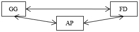
The variables used in this study are all endogenous, including GG, FD, and AP. The selection of these variables is based on references from literature reviews and identified research gaps discussed earlier. Furthermore, the endogeneity relationships of each variable in this study serve as the foundation, as illustrated in Figure 4.
Figure 4. Variable relationships
The operational definitions of the research variables have been summarized in Table 1.
Table 1. Operational definitions of research variables
|
Variable |
Indicator |
Unit |
Source |
|
GG |
The EG rate considers the depletion of natural resources, including net deforestation, energy, and mineral depletion. |
Persentase |
[24] |
|
FD |
Total FD in the short and long-term |
US Dollar |
[24] |
|
AP |
The number of people aged 65 and older |
Percentage of the total population |
[25] |
2.2 Data analysis methodology
This study employs the Vector Autoregression (VAR) approach, motivated by the types of variables and conceptual framework used in this research. In VAR analysis, there are no exogenous variables in the model, making all variables endogenous. The VAR approach is a reliable tool for describing data and making good predictions in multivariate equations [39]. Additionally, VAR examines how past values of a variable can explain its current state and are influenced by the past values observed from all other endogenous variables in the model. Moreover, VAR is commonly used to analyze relationships among a system of time series variables and the impact of shocks on the variable system. Based on this explanation, the econometric model for analyzing the endogeneity of GG, FD, and AP for comparison between Indonesia and Malaysia has been summarized in Eqs. (1) to (3).
GGt=α01i+∑ni=1β01iGGt−i+∑ni=1θ01iFDt−i+∑ni=1λ01iAPt−i+ε01t (1)
FDt=α02i+∑ni=1β02iGGt−i+∑ni=1θ02iFDt−i+∑ni=1λ02iAPt−i+ε02t (2)
APt=α03i+∑ni=1β03iGGt−i+∑ni=1θ03iFDt−i+∑ni=1λ03iAPt−i+ε03t (3)
Explanation:
t: time period
t−i: lagged time period i
α: constant
β,θ,λ: coefficients
ε: residual
Based on the explanation of the VAR approach concept, it is necessary to understand each stage of its operation to support the research objectives established [40]. The sequence of stages in implementing the VAR approach includes:
2.2.1 Stationarity test
Time series economic data generally exhibit stochastic properties or non-stationary trends, indicating the presence of unit roots in the data. To estimate the model using the data, it is essential to first test the stationarity of the data, known as the unit root test. The method used to determine whether variables in this study are stationary or not is through the unit root test.
2.2.2 Optimal lag
Determining the number of lags to use in the VAR model can be based on criteria such as Akaike Information Criterion (AIC) and Schwarz Information Criterion (SC). In this study, the lag chosen is the model with the lowest AIC value.
2.2.3 Stability test
To test the stability of the formed VAR estimation, a check is performed on the stability conditions of VAR, which involve the characteristics of polynomial roots. A VAR system is considered stable if the modulus of all its roots is less than 1.
2.2.4 Granger causality test
Causality testing can be performed using various methods, including Granger causality and error correction model causality. Granger causality is used to test the cause-effect relationship between two variables. The predictive power of previous information can indicate the presence of a cause-effect relationship between variables over time.
2.2.5 Cointegration test
If the stationary phenomenon is at the 1st difference level, then testing should be conducted to determine the possibility of cointegration. The concept of cointegration essentially ensures long-term equilibrium among the observed variables.
2.2.6 VAR instrument
VAR includes specific instruments capable of accounting for interactions among variables in the model. These instruments include Impulse Response Functions (IRF) and Variance Decompositions (VD). IRF applies a moving average vector to determine the impact of shocks in one variable on another. Meanwhile, VD is used to analyze the extent of shock impact on one variable to another.
3.1 Stationarity test results
The stationarity test for the data in this study employed a test called Augmented Dickey-Fuller (ADF). A variable is considered stationary if the probability value is less than α = 0.05. Conversely, a variable is deemed non-stationary if the probability value exceeds α = 0.05. However, if a categorical variable's data is found to be non-stationary, the solution involves employing non-stationary difference processes.
Table 2. Stationarity test results
|
Variable |
Indonesia |
|||
|
Level |
First Difference |
|||
|
ADF |
Prob |
ADF |
Prob |
|
|
GG |
-3.923001 |
0.0039 |
-15.19666 |
0.0000 |
|
FD |
-1.850967 |
0.3518 |
-3.790923 |
0.0260 |
|
AP |
-1.079824 |
0.9197 |
-5.207062 |
0.0007 |
|
Variable |
Malaysia |
|||
|
Level |
First Difference |
|||
|
ADF |
Prob |
ADF |
Prob |
|
|
GG |
-2.030760 |
0.2731 |
-8.435826 |
0.0000 |
|
FD |
1.926553 |
0.9998 |
-5.939257 |
0.0000 |
|
AP |
1.406892 |
0.9988 |
-3.531353 |
0.0116 |
Source: Author's work, 2024.
Table 2 summarizes the stationarity test results for the endogeneity models GG, FD, and AP comparing Indonesia and Malaysia at the level and first difference levels. From the table, it can be observed that the ADF probability value for the GG variable in Indonesia indicates stationarity at the level, as its probability is less than α = 0.05. However, the other variables for Indonesia and all variables for Malaysia are non-stationary at the level. Upon identifying these conditions, the ADF test procedure was then applied to test the stationarity of the variables by conducting unit root tests at the first difference level. Subsequently, from the results of the next stage of unit root tests, all variables in Indonesia and Malaysia, which previously did not pass at the level, were found to be stationary at the first difference level.
3.2 Optimal lag results
The VAR approach is highly sensitive to the number of lagged data used, hence it is essential to determine the optimal lag length. Determining this lag length helps in understanding the duration of influence periods on an endogenous variable both in the past and on other endogenous variables. The optimal lag length can be determined based on values of the likelihood ratio (LR), final prediction error (FPE), Akaike Information Criteria (AIC), Schwarz Criteria (SC), and Hannan-Quinn (HQ). These values can be found in Table 3.
Table 3. Optimal lag test results
|
Indonesia |
||||||
|
Lag |
LogR |
LR |
FPE |
AIC |
SC |
HQ |
|
0 |
-1103.098 |
NA |
4.42e+18 |
51.44643 |
51.56930 |
51.49174 |
|
1 |
-1041.255 |
112.1812 |
3.79e+17 |
48.98859 |
49.48009 |
49.16984 |
|
2 |
-1024.837 |
27.49090 |
2.70e+17 |
48.64356 |
49.50368 |
48.96075 |
|
3 |
-996.0618 |
44.16601 |
1.10e+17 |
47.72380 |
48.95255* |
48.17693 |
|
4 |
-983.3028 |
17.80324* |
9.51e+16* |
47.54897* |
49.14633 |
48.13803* |
|
Malaysia |
||||||
|
Lag |
LogR |
LR |
FPE |
AIC |
SC |
HQ |
|
0 |
-1.013.708 |
NA |
2.13e+17 |
4.841.466 |
4.853.877 |
4.846.015 |
|
1 |
-9.012.857 |
2.034.304 |
1.55e+15 |
4.348.980 |
4.398.627 |
4.367.177 |
|
2 |
-8.844.378 |
28.07981* |
1.08e+15* |
43.11609* |
43.98492* |
43.43455* |
|
3 |
-8.756.110 |
1.345.045 |
1.11e+15 |
4.312.433 |
4.436.552 |
4.357.928 |
|
4 |
-8.667.587 |
1.222.450 |
1.15e+15 |
4.313.137 |
4.474.492 |
4.372.280 |
Source: Author's work, 2024.
Table 3 summarizes the optimal lag test results. From the table, it is observed that the smallest AIC value (indicated by an asterisk) is at lag 4 for Indonesia, while for Malaysia, it is at lag 2. Therefore, the chosen optimal lag results for this study are lag 4 for Indonesia and lag 2 for Malaysia, based on the smallest AIC values.
3.3 Stability test results
Stability testing is necessary to determine whether the estimated VAR model is stable or not, based on the roots of the characteristic polynomial. A VAR model is considered stable if all its roots have moduli less than 1, a condition that can be observed in Table 4.
Table 4. Stability test results
|
Indonesia |
|
|
Root |
Modulus |
|
0.864388 - 0.108255i |
0.871140 |
|
0.864388 + 0.108255i |
0.871140 |
|
-0.202138 - 0.391418i |
0.440532 |
|
-0.202138 + 0.391418i |
0.440532 |
|
0.270478 |
0.270478 |
|
-0.235795 |
0.235795 |
|
Malaysia |
|
|
Root |
Modulus |
|
-0.248625 - 0.583660i |
0.634408 |
|
-0.248625 + 0.583660i |
0.634408 |
|
-0.380654 - 0.162513i |
0.413893 |
|
-0.380654 + 0.162513i |
0.413893 |
|
0.339853 |
0.339853 |
|
0.064719 |
0.064719 |
Source: Author's work, 2024.
Table 4 summarizes the stability test results for the endogeneity models GG, FD, and AP comparing Indonesia and Malaysia. From the table, there are no characteristic roots with moduli greater than 1 for both Indonesia and Malaysia. Additionally, from Figure 5, it is evident that all inverse roots of the AR polynomial are located inside the unit circle.
Figure 5. VAR stability test results
Source: Author's work, 2024.
3.4 Granger causality test results: How does endogeneity affect the relationship between GG, FD, and AP in Indonesia and Malaysia?
The Granger causality test among the variables in the study is conducted to determine the causal relationship between variables, which can be observed in Table 5.
Table 5. Granger causality test results
|
Indonesia |
|||
|
Null Hypothesis: |
Obs |
F-Statistic |
Prob. |
|
FD does not Granger Cause GG |
44 |
0.47239 |
0.7556 |
|
GG does not Granger Cause FD |
4.38016 |
0.0056 |
|
|
AP does not Granger Cause GG |
44 |
1.24405 |
0.3104 |
|
GG does not Granger Cause AP |
0.77663 |
0.5479 |
|
|
AP does not Granger Cause FD |
44 |
7.88443 |
0.0001 |
|
FD does not Granger Cause AP |
5.46479 |
0.0016 |
|
|
Malaysia |
|||
|
Null Hypothesis: |
Obs |
F-Statistic |
Prob. |
|
FD does not Granger Cause GG |
45 |
1.00107 |
0.3765 |
|
GG does not Granger Cause FD |
|
3.76295 |
0.0318 |
|
AP does not Granger Cause GG |
45 |
2.82557 |
0.0711 |
|
GG does not Granger Cause AP |
|
0.44707 |
0.6427 |
|
AP does not Granger Cause FD |
45 |
4.09229 |
0.0242 |
|
FD does not Granger Cause AP |
|
3.44567 |
0.0416 |
Source: Author's work, 2024.
Firstly, the Granger causality test conditions for both countries reveal that there are variables with bidirectional relationships, namely AP and FD. This indicates that AP influences FD and vice versa. Several factors contribute to the causal link between an AP and FD in Indonesia and Malaysia, primarily involving rising social expenditure. With the growing number of elderly individuals, the financial demands on the government budget increase. If domestic tax revenues fall short of meeting these demands, the government might resort to borrowing from foreign sources to address the budget shortfall. The influence of AP on FD tends to compel the government to increase spending in the health and social sectors, such as pensions, healthcare services, and long-term care. This can lead to larger budget deficits, forcing the government to borrow money from abroad. On the other hand, AP tends to reduce consumption due to lower pension income or financial uncertainty, potentially dampening long-term EG through lower domestic demand, which may prompt the government to take on more FD to stimulate EG. In line with this, the phenomenon of AP presents challenges for the government in financing long-term investments and innovations crucial for long-term EG. These resource constraints may drive the government to seek additional funding sources from abroad. Conversely, the influence of FD on AP suggests that higher FD restricts the government's ability to allocate public funds to social and healthcare services crucial for AP, such as elderly-friendly housing, healthcare facilities, and accessible public transportation. This could result in limited access to necessary healthcare for AP, thereby impacting their health and life expectancy. Furthermore, high FD tends to compel the government to reduce funds allocated to pension and social programs essential for AP, thereby diminishing their quality of life, potentially forcing them to work longer or rely on family resources. Based on these explanations, this research finding is supported by Gouriéroux et al. [41], suggesting that FD tends to burden a country's economy, reducing its capacity to invest in long-term EG. Insufficient investment in EG can hinder job creation needed to support AP's needs.
Secondly, there is a one-way relationship for both countries, where only GG influences FD because the implementation of GG tends to allocate more investment towards environmentally friendly infrastructure such as renewable energy, public transportation, and clean water management, which require FD to fund these large-scale projects. Elements that explain the link between GG and FD in Indonesia and Malaysia can be seen through the lens that effective GG projects can enhance investor confidence and generate new economic prospects, potentially affecting foreign debt patterns. When investors perceive opportunities for sustainable development, they might be more willing to offer financial support. Moreover, by focusing on energy efficiency and environmentally friendly technologies, GG can reduce dependence on energy imports, thus decreasing the trade balance deficit and potentially increasing FD for GG expansion. Additionally, implementing GG makes a country more proactive in the international community regarding climate change and sustainable development, thereby potentially accessing FD sources with low interest rates. Based on these explanations, this research finding is supported by Yared [42], suggesting that GG can provide long-term benefits in managing natural resources and enhancing environmental resilience, with proper implementation and wise FD management remaining crucial.
Thirdly, GG and AP do not influence each other in Indonesia due to their differing policy focuses and priorities. GG primarily focuses on transitioning to a more sustainable and environmentally friendly economy, aiming to improve resource efficiency and reduce environmental impact. On the other hand, AP reflects changes in the age structure of the population, with an increasing proportion of elderly individuals living longer. GG is often associated with technological innovation and environmental policies, whereas AP results from declining birth rates and increased life expectancy, which can occur independently of each other. Furthermore, GG tends to involve policy changes and medium- to long-term investments, while AP is a demographic process that unfolds gradually over several decades. For example, better environmental policies through GG can contribute to the health and well-being of AP, while GG through green technology development can create new economic opportunities crucial for AP. Nevertheless, directly, both tend to have their own distinct dynamics and can operate in parallel without directly influencing each other. Based on these explanations, this research finding is supported by Jahanger et al. [43], suggesting that the effects of GG are not directly felt or do not directly influence the dynamics of ongoing AP.
Fourthly, only AP influences GG in Malaysia because AP tends to prefer environmentally friendly or sustainable products and services. For instance, there may be an increased demand for renewable energy technologies or better public transportation as AP grows, thereby driving growth in these sectors through GG. Furthermore, AP typically has greater healthcare and welfare needs. These needs can motivate investments in more efficient and environmentally friendly healthcare infrastructure as part of GG, such as energy-efficient hospitals or more efficient medical technologies. Moreover, AP can generate increased demand for jobs in sectors related to elderly care, such as healthcare, social services, or technologies that help maintain their quality of life. This can stimulate GG through the creation of new jobs and increased productivity. Based on these explanations, this research finding is supported by Hosan et al. [44], suggesting that AP can present demographic and social challenges but also opportunities to promote GG through technological innovation, policy changes, and increased demand for environmentally friendly solutions.
3.5 Cointegration test results
This study employed the Johansen test by comparing the trace statistic with critical values at the α = 0.05 level. If the trace statistic is smaller than the critical value, then the two variables are not cointegrated, which can be seen in Table 6.
Table 6 summarizes the cointegration test results for Indonesia and Malaysia, where the trace statistic values appear to be smaller than the critical values for both countries. Thus, indicating that all variables are not cointegrated, meaning they do not have long-term relationships.
Table 6. Granger cointegration test results
|
Indonesia |
||||
|
Hypothesized No. of CE(s) |
Eigenvalue |
Trace Statistic |
0.05 Critical Value |
Prob.** |
|
None |
0.040482 |
6.692372 |
29.79707 |
0.9995 |
|
At most 1 |
0.007273 |
1.072250 |
15.49471 |
0.9999 |
|
At most 2 |
0.000585 |
0.079534 |
3.841466 |
0.7779 |
|
Malaysia |
||||
|
Hypothesized No. of CE(s) |
Eigenvalue |
Trace Statistic |
0.05 Critical Value |
Prob.** |
|
None |
0.408971 |
17.35436 |
27.58434 |
0.5497 |
|
At most 1 |
0.329991 |
13.21530 |
21.13162 |
0.4326 |
|
At most 2 |
0.149908 |
5.359549 |
14.26460 |
0.6959 |
Source: Author's work, 2024.
3.6 Results of VAR instrument test
The VAR analysis not only examines the endogeneity relationships among variables but also includes features like IRF and VD. These features allow for assessing how variables respond and the time required to return to their equilibrium points, as well as determining the extent of influence each variable has.
3.6.1 IRF results
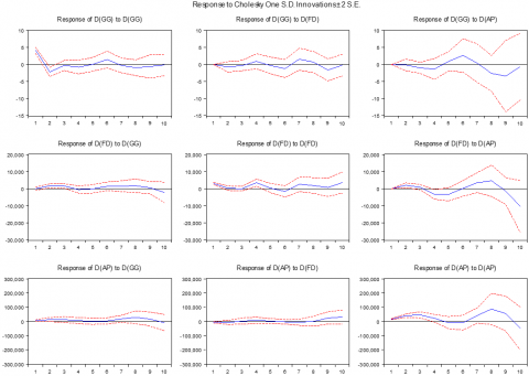
IRF provides an overview of how a variable responds in the future if there is a disturbance in another variable, presenting the analysis results in graphical form over 10 periods for easier interpretation. This test yields graphs illustrating whether the response of the variables is positive or negative. The IRF analysis results for the endogeneity of GG, FD, and AP in Indonesia and Malaysia can be viewed in Figures 6 and 7.
Based on the information in Figure 6 there are several main points, including FD in responding to shocks from GG in the response panel of D(GG) to D(FD) for 10 months, where FD tends to respond negatively to GG shocks except in the fourth and seventh months and getting closer to the point of equilibrium until the end of the period. This is different from AP in responding to shocks from GG in the response panel of D(GG) to D(AP) for 10 months, where AP tends to respond negatively to GG shocks except in the sixth month and gets closer to the balance point until the end of the period. Apart from that, GG responded to the shock from FD in the response panel of D(FD) to D(GG) for 10 months, where GG tended to respond positively to the FD shock except in the fourth and fifth months and further away from the balance point with a negative response until the end of the period. Then, AP responded to the shock from FD in the response panel of D(FD) to D(AP) for 10 months, where AP tended to respond positively to the FD shock except in the fourth and fifth months, and increasingly moved away from the balance point with a negative response until the end of the period. On the other hand, GG responded to a shock from AP in the response panel of D(AP) to D(GG) for 10 months, where GG received a positive shock from AP, and reached an equilibrium point at the end of the period. Finally, FD responded to a shock from AP in the response panel of D(AP) to D(FD) for 10 months, where FD tended to respond positively to AP shocks and moved further away from the equilibrium point at the end of the period.
Figure 6. IRF analysis results for Indonesia
Source: Author's work, 2024.
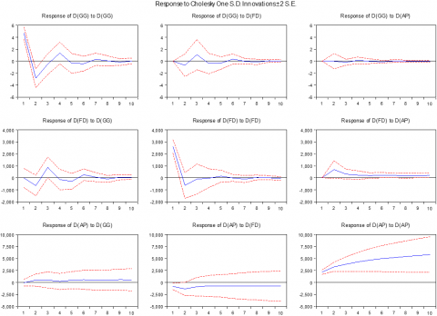
Figure 7. IRF analysis results for Malaysia
Source: Author's work, 2024.
Based on the information in Figure 7 there are several main points, including FD in responding to shocks from GG in the response panel of D(GG) to D(FD) for 10 months, where FD tends to respond positively to GG shocks except in the third and sixth months and getting closer to the point of equilibrium until the end of the period. This is different from AP in responding to shocks from GG in the response panel of D(GG) to D(AP) for 10 months, where AP tends to respond negatively to GG shocks except in the third and sixth months and gets closer to the balance point until the end of the period. Apart from that, GG responded to the shock from FD in the response panel of D(FD) to D(GG) for 10 months, where GG tended to respond negatively to the FD shock except in the third and sixth months and was getting closer to the balance point with a negative response. until the end of the period. Then, AP responded to the shock from FD in the response panel of D(FD) to D(AP) for 10 months, where AP tended to respond positively to the FD shock, and was getting closer to the point of balance until the end of the period. On the other hand, GG responded to a shock from AP in the response panel of D(AP) to D(GG) for 10 months, where GG received a positive shock from AP, and approached the equilibrium point at the end of the period. Finally, FD responded to a shock from AP in the response panel of D(AP) to D(FD) for 10 months, where FD tended to respond negatively to AP shocks and got closer to the balance point at the end of the period.
3.6.2 VD results
VD complements previous analysis by providing estimates of how much each variable contributes to the changes in itself and other variables over several future periods, measured in percentage terms. This allows us to understand which variables are expected to have the largest contributions to a specific variable. The VD results in this study can be seen in Tables 7-9.
Table 7. VD results for D(GG)
|
Indonesia |
||||
|
Period |
S.E. |
D(GG) |
D(FD) |
D(AP) |
|
1 |
4.134733 |
100.0000 |
0.000000 |
0.000000 |
|
2 |
4.729798 |
97.60764 |
2.304919 |
0.087439 |
|
3 |
4.850724 |
93.18216 |
2.689695 |
4.128141 |
|
4 |
5.186135 |
83.93970 |
5.543283 |
10.51701 |
|
5 |
5.275425 |
81.12870 |
5.708159 |
13.16315 |
|
6 |
6.197846 |
64.14242 |
7.962709 |
26.50690 |
|
7 |
6.403623 |
60.27564 |
11.96876 |
27.89487 |
|
8 |
7.016789 |
52.08739 |
13.21746 |
35.94385 |
|
9 |
7.999279 |
40.64971 |
13.32390 |
45.99373 |
|
10 |
8.025633 |
40.41052 |
13.35656 |
46.26558 |
|
Malaysia |
||||
|
Period |
S.E. |
D(GG) |
D(FD) |
D(AP) |
|
1 |
4.711124 |
100.0000 |
0.000000 |
0.000000 |
|
2 |
5.542816 |
98.50752 |
1.492406 |
0.079504 |
|
3 |
5.671968 |
94.80323 |
5.081913 |
0.114858 |
|
4 |
5.849480 |
94.58418 |
5.246027 |
0.169793 |
|
5 |
5.869754 |
94.34374 |
5.487154 |
0.169109 |
|
6 |
5.895305 |
94.52154 |
5.792937 |
0.195525 |
|
7 |
5.903433 |
94.41602 |
5.778240 |
0.195737 |
|
8 |
5.905182 |
93.07823 |
5.826124 |
0.195645 |
|
9 |
5.907781 |
93.06393 |
5.834647 |
0.201423 |
|
10 |
5.908011 |
93.05951 |
5.837706 |
0.202786 |
Source: Author's work, 2024.
Table 7 summarizes the VD results for D(GG) in Indonesia and Malaysia, indicating that the variables expected to have the largest contributions to GG in the next 10 months differ between the two countries. For Indonesia, the variable expected to contribute the most to GG is GG itself, with an average monthly contribution of 71.34%, followed by AP with 21.05% and FD with 7.61%. For Malaysia, the variable expected to contribute the most to GG is also GG itself, with an average monthly contribution of 95.22%, followed by FD with 4.64% and AP with 0.14%. Based on this explanation, in both countries, GG provides the highest average monthly contribution, but its monthly contributions are decreasing over time. Conversely, FD and AP have smaller average monthly contributions initially but show increasing contributions over time.
Table 8. VD results for D(FD)
|
Indonesia |
||||
|
Period |
S.E. |
D(GG) |
D(FD) |
D(AP) |
|
1 |
3104.272 |
0.029722 |
99.97028 |
0.000000 |
|
2 |
4077.892 |
11.63626 |
58.44401 |
23.13379 |
|
3 |
4471.067 |
11.65141 |
50.92103 |
24.18833 |
|
4 |
6618.442 |
12.04871 |
48.62093 |
24.38513 |
|
5 |
7418.051 |
12.05933 |
41.94521 |
45.29546 |
|
6 |
7717.213 |
12.31692 |
40.75601 |
48.67603 |
|
7 |
8985.401 |
12.94518 |
39.27526 |
48.92706 |
|
8 |
10437.28 |
17.17086 |
32.25296 |
56.09562 |
|
9 |
10569.60 |
27.19074 |
31.90433 |
56.45941 |
|
10 |
15320.85 |
30.81290 |
20.74591 |
71.77279 |
|
Malaysia |
||||
|
Period |
S.E. |
D(GG) |
D(FD) |
D(AP) |
|
1 |
2613.408 |
0.000546 |
99.99945 |
0.000000 |
|
2 |
2849.536 |
13.10179 |
89.03919 |
5.790377 |
|
3 |
2997.649 |
13.23857 |
80.57897 |
6.319245 |
|
4 |
3009.869 |
14.02016 |
79.93734 |
6.824096 |
|
5 |
3034.065 |
14.47631 |
78.87596 |
7.103875 |
|
6 |
3052.544 |
14.50136 |
77.92598 |
7.517467 |
|
7 |
3061.304 |
14.51138 |
77.59723 |
7.901416 |
|
8 |
3067.625 |
14.54187 |
77.28521 |
8.172924 |
|
9 |
3073.630 |
14.55656 |
76.98355 |
8.505063 |
|
10 |
3080.589 |
15.17043 |
76.66480 |
8.858894 |
Source: Author's work, 2024.
Table 8 summarizes the Variance Decomposition (VD) results for D(FD) in Indonesia and Malaysia, showing the variables expected to have the largest contributions to FD in the next 10 months differ between the two countries. For Indonesia, the variable expected to contribute the most to FD is FD itself, with an average monthly contribution of 46.48%, followed by AP at 39.89% and GG at 14.79%. For Malaysia, the variable expected to contribute the most to FD is also FD itself, with an average monthly contribution of 81.49%, followed by GG with 12.81% and AP with 6.69%. Based on this explanation, in both countries, FD provides the highest average monthly contribution, but its monthly contributions are decreasing over time. Conversely, GG and AP have smaller average monthly contributions initially but show increasing contributions over time.
Table 9 summarizes the Variance Decomposition (VD) results for D(AP) in Indonesia and Malaysia, indicating the variables expected to have the largest contributions to AP in the next 10 months differ between the two countries. For Indonesia, the variable expected to contribute the most to AP is AP itself, with an average monthly contribution of 87.13%, followed by GG with 9.20% and FD with 3.79%. For Malaysia, the variable expected to contribute the most to AP is also AP itself, with an average monthly contribution of 92.05%, followed by FD with 6.99% and GG with 1.02%. Based on this explanation, in both countries, AP provides the highest average monthly contribution, but its monthly contributions are decreasing over time. Conversely, GG and FD have smaller average monthly contributions initially but show increasing contributions over time.
Table 9. VD results for D(AP)
|
Indonesia |
||||
|
Period |
S.E. |
D(GG) |
D(FD) |
D(AP) |
|
1 |
17762.88 |
8.096784 |
1.259014 |
89.71060 |
|
2 |
47180.73 |
8.211903 |
1.803667 |
88.81664 |
|
3 |
67495.45 |
8.265662 |
2.690083 |
88.79735 |
|
4 |
71979.22 |
8.485731 |
2.990750 |
88.59665 |
|
5 |
72569.52 |
8.600741 |
3.086580 |
88.56005 |
|
6 |
73173.50 |
9.640204 |
3.137690 |
86.95373 |
|
7 |
86235.79 |
9.716316 |
3.329950 |
86.85247 |
|
8 |
126666.3 |
10.45745 |
4.024529 |
86.33527 |
|
9 |
141406.1 |
10.33536 |
6.799963 |
83.76509 |
|
10 |
152572.1 |
10.18094 |
7.634172 |
82.86468 |
|
Malaysia |
||||
|
Period |
S.E. |
D(GG) |
D(FD) |
D(AP) |
|
1 |
2319.299 |
0.065042 |
9.870774 |
95.80752 |
|
2 |
4251.271 |
0.960313 |
7.331290 |
95.52974 |
|
3 |
5802.821 |
0.974258 |
5.829880 |
95.19061 |
|
4 |
7259.099 |
0.975549 |
4.963641 |
94.67204 |
|
5 |
8676.870 |
1.005457 |
4.322500 |
93.95238 |
|
6 |
10043.05 |
1.039257 |
3.835133 |
93.13086 |
|
7 |
11337.79 |
1.053513 |
3.494716 |
91.61520 |
|
8 |
12591.29 |
1.083982 |
3.232170 |
88.60190 |
|
9 |
13819.14 |
1.373567 |
13.98470 |
86.88343 |
|
10 |
15019.63 |
1.527327 |
13.05153 |
84.64174 |
Source: Author's work, 2024.
Based on the endogeneity analysis conducted, the findings of this study highlight similar and different results in the comparisons made as a novelty of the study. The novel contribution of this study is to obtain consistent findings in both countries covering the causality between AP and FD, with only GG affecting FD. These consistent findings indicate coherence among the analyzed countries, thus supporting the generalization of the research outcomes. In other words, the findings of this study have potential relevance for other countries with similar characteristics within the same context. Moreover, this consistency reinforces confidence in the validity of the research findings, suggesting that observed patterns or relationships are less likely influenced by specific factors of any country. Therefore, this provides a stronger foundation for developing universally applicable policies to design more effective strategies in a global or regional context. Furthermore, there are also differing findings between the two countries. In Malaysia, only AP affects GG, whereas in Indonesia, there is no significant relationship between AP and GG, even though it is unidirectional. This means that the relationships studied cannot be considered uniform across both countries and require a more contextual approach in interpretation. Additionally, specific factors in the investigated countries have different influences on the phenomena studied, indicating that the findings of this research cannot be broadly applied and present opportunities for further research to delve into factors that may influence these differences.
There are two policy recommendations from this research that are generalizable to the analyzed countries. First, governments need to manage FD and address AP in the context of sustainable development through prudent FD management to ensure that FD is used for productive investments that can enhance economic growth in the long term. This includes transparency in loan utilization, diversification of funding sources, and careful risk management. Furthermore, such FD management will promote investment in inclusive and sustainable healthcare systems to address AP needs. This encompasses better access to primary healthcare, geriatric services, and financial protection. Additionally, FD management can also be focused on developing education and training programs to enhance AP skills and adaptability, thereby maintaining their productivity in the labor market. Second, governments need to incentivize GG to significantly contribute to FD in the context of sustainable development by providing fiscal incentives such as tax exemptions or tax credits for investments in green technologies and eco-friendly infrastructure projects. This can enhance GG and attract private investments that can reduce reliance on FD. Moreover, governments need to enhance resource efficiency and energy savings through energy-efficient production practices, which not only reduce operational costs but also lessen dependence on energy imports and help manage trade deficits that can affect FD.
Furthermore, there are also policy recommendations from this research specific to Malaysia. The government needs to manage environmental governance to promote GG in the context of sustainable development through fiscal incentives such as tax exemptions or tax credits for companies investing in green technology and environmentally friendly infrastructure projects. On the other hand, it is also crucial for the government to develop education and training programs tailored to environmental professionals, empowering them with new skills relevant to the green sector.
This research has several weaknesses that need to be considered for future studies. Among these, the endogeneity approach often captures complex and mutually influencing relationships between the variables under study. However, in the context of GG, FD, and AP, there is a risk that the relationship between these variables may be influenced by unobserved or poorly controlled factors in the analysis. Therefore, it is necessary to consider other exogenous variables for each endogenous variable in this study to make it more comprehensive.
This work is supported by the Padang State University from the Special Research Scheme for Professors (Grant No.: 1433/UN35.15/LT/2024).
[1] Chen, J., Wang, Y., Wen, J., Fang, F., Song, M. (2016). The influences of aging population and economic growth on Chinese rural poverty. Journal of Rural Studies, 47: 665-676. https://doi.org/10.1016/j.jrurstud.2015.11.002
[2] Aimon, H., Kurniadi, A.P., Amar, S. (2021). Analysis of fuel oil consumption, green economic growth and environmental degradation in 6 Asia Pacific countries. International Journal of Sustainable Development and Planning, 16(5): 925-933. https://doi.org/10.18280/ijsdp.160513
[3] Kurniadi, A.P., Aimon, H., Amar, S. (2022). Analysis of green economic growth, biofuel oil consumption, fuel oil consumption and carbon emission in Asia Pacific. International Journal of Sustainable Development & Planning, 17(7): 2247-2254. https://doi.org/10.18280/ijsdp.170725
[4] Ince Yenilmez, M. (2015). Economic and social consequences of population aging the dilemmas and opportunities in the twenty-first century. Applied Research in Quality of Life, 10: 735-752. https://doi.org/10.1007/s11482-014-9334-2
[5] Herrmann, M. (2012). Population aging and economic development: Anxieties and policy responses. Journal of Population Ageing, 5: 23-46. https://doi.org/10.1007/s12062-011-9053-5
[6] Pirog, M.A. (2018). The economics and policy ramifications of an aging population. Contemporary Economic Policy, 36(3): 431-435. https://doi.org/10.1111/coep.12389
[7] Pham, T.N., Vo, D.H. (2021). Aging population and economic growth in developing countries: A quantile regression approach. Emerging Markets Finance and Trade, 57(1): 108-122. https://doi.org/10.1080/1540496X.2019.1698418
[8] Aimon, H., Kurniadi, A.P., Sentosa, S.U., Yahya, Y. (2024). What is the relationship between financial stability and economic growth in APEC? International Journal of Sustainable Development and Planning, 19(7): 2691-2698. https://doi.org/10.18280/ijsdp.190725
[9] Kurniadi, A.P., Aimon, H., Salim, Z., Ragimun, R., Sonjaya, A., Setiawan, S., Siagian, V., Nasution, L.Z., Nurhidajat, R., Mutaqin, M., Sabtohadi, J. (2024). Analysis of existing and forecasting for coal and solar energy consumption on climate change in Asia Pacific: New evidence for sustainable development goals. International Journal of Energy Economics and Policy, 14(4): 352-359. https://doi.org/10.32479/ijeep.16187
[10] Annisa, N., Taher, A.R.Y. (2022). The effect of foreign debt, labor force, and net exports on Indonesia's economic growth in period of 1986 Q1-2020 Q4. Jurnal Ekonomi Dan Bisnis Jagaditha, 9(1): 39-46. https://doi.org/10.22225/jj.9.1.2022.39-46
[11] Senadza, B., Fiagbe, K., Quartey, P. (2017). The effect of external debt on economic growth in Sub-Saharan Africa. International Journal of Business and Economic Sciences Applied Research, 11(1): 61-69, https://doi.org/10.25103/ijbesar.111.07
[12] Mohsin, M., Ullah, H., Iqbal, N., Iqbal, W., Taghizadeh-Hesary, F. (2021). How external debt led to economic growth in South Asia: A policy perspective analysis from quantile regression. Economic Analysis and Policy, 72: 423-437. https://doi.org/10.1016/j.eap.2021.09.012
[13] Ndubuisi, P. (2017). Analysis of the impact of external debt on economic growth in an emerging economy: Evidence from Nigeria. African Research Review, 11(4): 156-173. http://doi.org/10.4314/afrrev.v11i4.13
[14] Hopenhayn, H., Neira, J., Singhania, R. (2022). From population growth to firm demographics: Implications for concentration, entrepreneurship and the labor share. Econometrica, 90(4): 1879-1914. https://doi.org/10.3982/ECTA18012
[15] Rahman, M.M. (2017). Do population density, economic growth, energy use and exports adversely affect environmental quality in Asian populous countries? Renewable and Sustainable Energy Reviews, 77(C): 506-514. https://doi.org/10.1016/j.rser.2017.04.041
[16] Hashmi, R., Alam, K. (2019). Dynamic relationship among environmental regulation, innovation, CO2 emissions, population, and economic growth in OECD countries: A panel investigation. Journal of Cleaner Production, 231: 1100-1109. https://doi.org/10.1016/j.jclepro.2019.05.325
[17] Lopreite, M., Mauro, M. (2017). The effects of population ageing on health care expenditure: A Bayesian VAR analysis using data from Italy. Health Policy, 121(6): 663-674. https://doi.org/10.1016/j.healthpol.2017.03.015
[18] Kharusi, S.A., Ada, M.S. (2018). External debt and economic growth: The case of emerging economy. Journal of Economic Integration, 33(1): 1141-1157. https://doi.org/10.11130/jei.2018.33.1.1141
[19] Shkolnyk, I., Koilo, V. (2018). The relationship between external debt and economic growth: Empirical evidence from Ukraine and other emerging economies. Investment Management and Financial Innovations, 15(1): 387-400. http://doi.org/10.21511/imfi.15(1).2018.32
[20] N’Zue, F.F. (2020). Is external debt hampering growth in the ECOWAS region. International Journal of Economics and Finance, 12(4): 54-66. https://doi.org/10.5539/ijef.v12n4p54
[21] Buterin, V., Fajdetić, B., Mrvčić, M. (2022). Impact of migration and population aging on economic growth in the Republic of Croatia. Ekonomski vjesnik: Review of Contemporary Entrepreneurship, Business, and Economic Issues, 35(1): 151-164. https://doi.org/10.51680/ev.35.1.12
[22] Park, H., Son, J.C. (2021). Threshold effects of population aging on economic growth: A cross-country analysis. The Singapore Economic Review, 1-23. https://doi.org/10.1142/S021759082150034X
[23] Ruggerio, C.A. (2021). Sustainability and sustainable development: A review of principles and definitions. Science of the Total Environment, 786(147481): 1-11. https://doi.org/10.1016/j.scitotenv.2021.147481
[24] Tomislav, K. (2018). The concept of sustainable development: From its beginning to the contemporary issues. Zagreb International Review of Economics & Business, 21(1): 67-94. https://doi.org/10.2478/zireb-2018-0005
[25] World Bank. (2024). https://data.worldbank.org/.
[26] Federal Reserve Economic Data. (2024). https://fred.stlouisfed.org/.
[27] Anderu, K.S., Omolade, A., Oguntuase, A. (2019). External debt and economic growth in Nigeria. Journal of African Union Studies, 8(3): 157-171. https://doi.org/10.31920/2050-4306/2019/8n3a8
[28] Broner, F., Clancy, D., Erce, A., Martin, A. (2022). Fiscal multipliers and foreign holdings of public debt. The Review of Economic Studies, 89(3): 1155-1204. https://doi.org/10.1093/restud/rdab055
[29] Dey, S.R., Tareque, M. (2020). External debt and growth: Role of stable macroeconomic policies. Journal of Economics, Finance and Administrative Science, 25(50): 185-204. https://doi.org/10.1108/JEFAS-05-2019-0069
[30] Mohamed, A.N., Abdulle, A.Y. (2023). The asymmetric effects of government debt on GDP growth: Evidence from Somalia. International Journal of Sustainable Development and Planning, 18(8): 2403-2410. https://doi.org/10.18280/ijsdp.180811
[31] Maestas, N., Mullen, K.J., Powell, D. (2023). The effect of population aging on economic growth, the labor force, and productivity. American Economic Journal: Macroeconomics, 15(2): 306-332. https://doi.org/10.1257/mac.20190196
[32] McGrattan, E.R., Prescott, E.C. (2017). On financing retirement with an aging population. Quantitative Economics, 8(1): 75-115. https://doi.org/10.3982/QE648
[33] Kurniadi, A.P., Aimon, H., Amar, S. (2021). Determinants of biofuels production and consumption, green economic growth and environmental degradation in 6 Asia Pacific countries: A simultaneous panel model approach. International Journal of Energy Economics and Policy, 11(5): 460-471. https://doi.org/10.32479/ijeep.11563
[34] Aimon, H., Kurniadi, A.P., Sentosa, S.U., Abd Rahman, N. (2023). Production, consumption, export and carbon emission for coal commodities: Cases of Indonesia and Australia. International Journal of Energy Economics and Policy, 13(5): 484-492. https://doi.org/10.32479/ijeep.14798
[35] Aimon, H., Putri, K.A., Ulfa, S.S. (2022). Employment opportunities and income analysis before and during COVID-19: Indirect least square approach. Studies in Business and Economics, 17(2): 5-22. https://doi.org/10.2478/sbe-2022-0022
[36] Kurniasih, E.P. (2021). The effect of foreign debt on the economic growth. Jurnal Ekonomi Malaysia, 55(3): 125-136. https://doi.org/10.17576/JEM-2021-5503-09
[37] Yasar, N. (2021). The causal relationship between foreign debt and economic growth: Evidence from Commonwealth Independent States. Foreign Trade Review, 56(4): 415-429. https://doi.org/10.1177/00157325211018329
[38] Acemoglu, D., Restrepo, P. (2017). Secular stagnation? The effect of aging on economic growth in the age of automation. American Economic Review, 107(5): 174-179. https://doi.org/10.1257/aer.p20171101
[39] Mirzaie, M., Darabi, S. (2017). Population aging in Iran and rising health care costs. Iranian Journal of Ageing, 12(2): 156-169. https://doi.org/10.21859/sija-1202156
[40] Koop, G., Korobilis, D., Pettenuzzo, D. (2019). Bayesian compressed vector autoregressions. Journal of Econometrics, 210(1): 135-154. https://doi.org/10.1016/j.jeconom.2018.11.009
[41] Gouriéroux, C., Monfort, A., Renne, J.P. (2017). Statistical inference for independent component analysis: Application to structural VAR models. Journal of Econometrics, 196(1): 111-126. https://doi.org/10.1016/j.jeconom.2016.09.007
[42] Yared, P. (2019). Rising government debt: Causes and solutions for a decades-old trend. Journal of Economic Perspectives, 33(2): 115-140. https://doi.org/10.1257/jep.33.2.115
[43] Jahanger, A., Balsalobre-Lorente, D., Ali, M., Samour, A., Abbas, S., Tursoy, T., Joof, F. (2023). Going away or going green in ASEAN countries: Testing the impact of green financing and energy on environmental sustainability. Energy & Environment, pp. 1-26. https://doi.org/10.1177/0958305X231171346
[44] Hosan, S., Karmaker, S.C., Rahman, M.M., Chapman, A.J., Saha, B.B. (2022). Dynamic links among the demographic dividend, digitalization, energy intensity and sustainable economic growth: Empirical evidence from emerging economies. Journal of Cleaner Production, 330(129858): 1-15. https://doi.org/10.1016/j.jclepro.2021.129858