Thair Jabbar Mizhir AL-Fatlawi*![]() | Karrar Ghanim Hameed AL-Talebi
| Karrar Ghanim Hameed AL-Talebi![]()
© 2024 The authors. This article is published by IIETA and is licensed under the CC BY 4.0 license (http://creativecommons.org/licenses/by/4.0/).
OPEN ACCESS
A substantial subject for the hydrological cycle, engineers must be able to determine the amount of rainfall in order to design structures and dams that deal with collection, transport and storage runoff. The study provides information on the amount of rainfall (measured in millimeters) that occurred annually from 1991 to 2021 in a single meteorological station in Iraq, specifically Babylon. The distributions of observed frequency are described, and the study attempts to fit three theoretical distributions (Gamma, Log Normal, and Normal) to the data. The distributions and tests chosen for the study play crucial roles in statistical analysis. The Normal distribution, a fundamental pattern in statistics, helps identify common trends in data and is a key part of quality control processes. It is often taught early in statistical education due to its significance in understanding natural variations and environmental factors. The Gamma distribution is widely used in statistics to model time durations for tasks or events. The Log-Normal distribution describes a variable whose logarithm follows a normal distribution. Chi-square test is a statistical method to compare expected and observed outcomes across different categories, commonly employed in survey analysis. The Kolmogorov-Smirnov test compares distributions of two independent samples, useful for evaluating how well a theoretical distribution fits actual data. Researchers use this test under similar conditions as the Chi-square test. The Kolmogorov-Smirnov and Chi-Square and Anderson-Darling indices where, the calculated value of nonparametric test (statistic value) is extract and compared with the tabular value (critical value) based on the significant (α) and degrees of freedom, if the calculated value is less than the tabular value, we accept the null hypothesis (good fit); otherwise, we do not accept the null hypothesis (poor fit). They are used to compare the theoretical distributions to the observed data. The study then focuses on the Intensity-Duration-Frequency (IDF) curves for extreme rainfall values, with durations of 15, 30, and 60 minutes. The results reveal that rainfall intensity decreases as the duration of the storm increases. Additionally, rainfall of a specific duration shows higher intensity if the return period is greater. Gumbel’s extreme value distribution, Normal distribution, and Log Normal distribution are used to fit rainfall data with 5, 10, 15, and 50-year return periods. The Excel Software showed that the lognormal, normal, and Gamma probability distributions were the best fit for the data group for all durations. The software estimated the intensities of precipitation for return periods of 5, 10, 15, and 50 years, and the Log Normal distribution presented as the good agreement.
Intensity-Duration-Frequency (IDF), probability distributions, precipitation, Excel Software, Babylon City, normal distribution, Log Normal distribution, Gamma distribution
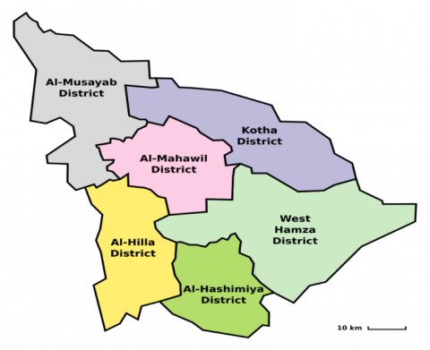
Rainfall is an important aspect of water resources that needs to be accurately measured. Hydrologic models require accurate estimates of mean rainfall [1]. Extreme rainfall events pose challenges to society in terms of human and economic impact and require a multidisciplinary approach to be analyzed. To construct hydraulic structures that manage stormwater runoff, it is essential to gather data on the amount of intense rainfall over different time periods. This information is typically represented through an Intensity-Duration-Frequency relationship [2]. Babylon City is situated in central Iraq, along the Babylon branch of the Euphrates River, approximately 100km south of Baghdad. The population of Babylon province is around 3,000,000 residents, with an annual growth rate of about 3%. Serving as the provincial capital, Babylon City is located adjacent to the ancient city of Babylon and in close proximity to the historic cities of Borsippa and Kish. Covering an area of 5116 km2, Babylon City is primarily characterized by agricultural activities. The region benefits from extensive irrigation facilitated by the Babylon canal, enabling the cultivation of diverse crops, fruits, and textiles. The river flows through the city center, flanked by date palm trees and other arid vegetation, which effectively mitigate the adverse effects of dust and desert winds.
IDF curve is a tool used in the design of hydraulic structures like drainage networks, bridges, and road culverts. It helps engineers estimate extreme rainfall levels by analyzing the frequency of occurrence for different durations. This is done through a technique called frequency analysis (FA), which involves fitting a probability distribution to the recorded rainfall intensities. By using this approach, engineers can determine the appropriate design parameters to ensure the structures can withstand extreme weather conditions [3]. The study estimated the likelihood of an event occurring every 100 years for combinations of annual maximum rainfall measurements collected from rain gauges in Southeastern Arizona using different frequency distributions and methods. The Log Normal distribution can be successfully used to fit a straight line through the upper data points for durations ranging from 5 to 120 minutes. Fitting thunderstorm rainfall data through mathematical or visual methods may lead to errors in estimating 100-year rainfall depths, with mathematical fitting more likely to overestimate. These graphs continue to be analyzed by researchers interested in climate and hydrological risk [4]. Used the magnitude of annual flood peak maxima at 152 representative sites totaling 6728 years of record were obtained from department of water affairs and forestry. The value of 50 year design flood by using three distribution obtained (Log Pearson type III, Generalized extreme value, and Extreme value type I distributions), the statistical analysis confirm that the widely used Log Pearson type III distribution using conventional moments estimators. The Gumbel distribution is commonly utilized to represent various time intervals of yearly maximum precipitation in a singular FA framework. This method presumes that the various durations are autonomous and frequently incorporates simplifications, which have been utilized by numerous authors and services to establish IDF curves for extreme precipitation [5]. Estimated one day and two to five consecutive days annual maximum rainfall of various return periods from 2 to 100 years at In Banswara, Rajasthan, India, researchers used three probability distributions (Normal, Log Normal, and Gamma) to analyze the data and determine the best fit. They compared the distributions using the Chi-square value and conducted frequency analysis using a frequency factor. The findings revealed that the Normal distribution function was the most suitable for predicting rainfall patterns for one, two, and three consecutive days. On the other hand, the Gamma distribution function provided the best fit for four and five consecutive days [6].
In another study conducted in the city of London, researchers developed IDF curves for three different weather scenarios: historic, wet, and dry. They utilized rainfall data collected by the Meteorological Service of Canada from 1943 to 2001. The rainfall data was gathered for various durations, ranging from as short as 5 minutes to as long as 24 hours. The researchers extracted extreme values for each duration from the time series data and fitted them to Gumbel's extreme value distribution. This analysis is crucial for assessing water availability for agriculture, industry, and other human activities, as rainfall serves as a vital factor in these sectors.
Understanding how rainfall is distributed in time and space is vital for a country's economy. Instead of relying solely on summary statistics, having knowledge of the actual distribution of precipitation greatly enhances various applications of rainfall data. Researchers have conducted numerous studies to explore different methods of representing real rainfall patterns for specific purposes [7].
Rainfall curves, also known as IDF curves, provide insights into the amount of water that falls within a specific timeframe. These curves are valuable for predicting potential flooding in an area or calculating the duration and volume of rainfall. To analyze extreme rainfall events and make predictions about future water flow, it is essential to examine the relationship between different duration levels. Multivariate models offer a promising approach to investigate this significant question. Among these models, the copula theory has gained widespread application in hydrometeorology [8]. The research aims to analyze the uncertainty in IDF curves for Babylon City to determine the expected rainfall. With extreme rainfall events becoming more frequent, the risk of flooding is on the rise. It's crucial to upgrade stormwater drainage systems in urban areas to handle these increasing extreme rainfall events. Currently, historical IDF curves are vital for designing these drainage systems. Hence, there is an urgent call to review the existing IDF curves essential for urban rainwater drainage design. This study addresses flood risk by developing rainwater harvesting systems to manage rainfall effectively (Figure 1).
Figure 1. The studied zone location
There are the methods to estimate data using theoretical distributions.
These methods are:
1) Fitting by mathematical method
Statistical analysis often involves the use of various probability distributions. In this paper, three distributions are considered: Normal, Log Normal, and Gamma distributions. To estimate the parameters of these distributions, researchers employ either the moments method or the maximum likelihood method. Typically, the parameters of the statistical model are derived from a sample using either the moments estimation method or maximum likelihood estimates. Once the parameter values are obtained, they are substituted into the selected distribution function to calculate probabilities [9].
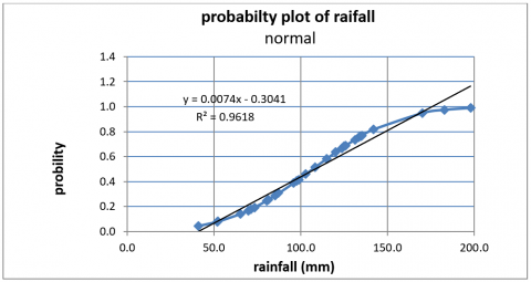
Tables 1 and 2 display probability estimates using the moments method for all chosen distributions at Babylon station, while Figure 2 depicts the frequency curve for the Normal distribution.
Table 1. An overview of the statistical distributions and their corresponding functions analyzed in this study
|
Statistical Distributions |
Functions |
|
Normal distribution |
$f(x)=\frac{1}{\sqrt{2 \pi \sigma^2}} \exp \left(\frac{-(x-\mu)^2}{2 \sigma^2}\right)$ |
|
Log Normal distribution |
$f(x)=\frac{1}{\sqrt{2 \pi \sigma_{\mathrm{x}}^2}} \exp \left(-\frac{\left(\log \mathrm{x}-\mu_{\mathrm{y}}\right)^2}{2 \sigma^2 \mathrm{y}}\right)$ |
|
Gamma distribution |
$f(x)=\frac{\lambda^\beta x^{(\beta-1)} e^{-\lambda_x}}{\Gamma(\beta)}$ |
Figure 2. Frequency curve with respect to the Normal dis. (moments method) for Babylon station
Table 2. Estimations of probabilities by moments method (Babylon station), Iraqi Meteorological Office in Baghdad, Iraq
|
Total Rainfall (mm) |
Ln($\chi$) |
Rank(m) |
Normal F(x) % |
Log Normal F(x) % |
Gamma F(x) % |
|
41.0 |
3.71 |
1 |
4.410 |
0.315 |
1.544 |
|
51.8 |
3.95 |
2 |
7.703 |
1.949 |
4.829 |
|
52.4 |
3.96 |
3 |
7.932 |
2.112 |
5.091 |
|
65.3 |
4.18 |
4 |
14.102 |
8.034 |
12.828 |
|
69.8 |
4.25 |
5 |
16.872 |
11.267 |
16.455 |
|
71.1 |
4.26 |
6 |
17.734 |
12.308 |
17.582 |
|
73.2 |
4.29 |
7 |
19.183 |
14.083 |
19.470 |
|
80.3 |
4.39 |
8 |
24.596 |
20.838 |
26.390 |
|
81.3 |
4.40 |
9 |
25.419 |
21.867 |
27.419 |
|
85.3 |
4.45 |
10 |
28.849 |
26.125 |
31.628 |
|
87.3 |
4.47 |
11 |
30.644 |
28.324 |
33.779 |
|
95.8 |
4.56 |
12 |
38.750 |
37.911 |
43.052 |
|
97.6 |
4.58 |
13 |
40.548 |
39.951 |
45.012 |
|
98.7 |
4.59 |
14 |
41.655 |
41.192 |
46.202 |
|
102.8 |
4.63 |
15 |
45.837 |
45.766 |
50.588 |
|
108.2 |
4.68 |
16 |
51.409 |
51.593 |
56.171 |
|
114.7 |
4.74 |
17 |
58.070 |
58.185 |
62.493 |
|
120.1 |
4.79 |
18 |
63.443 |
63.236 |
67.344 |
|
123.5 |
4.82 |
19 |
66.700 |
66.197 |
70.190 |
|
125.0 |
4.83 |
20 |
68.100 |
67.449 |
71.393 |
|
125.7 |
4.83 |
21 |
68.744 |
68.022 |
71.943 |
|
131.1 |
4.88 |
22 |
73.515 |
72.189 |
75.946 |
|
133.4 |
4.89 |
23 |
75.429 |
73.832 |
77.522 |
|
134.5 |
4.90 |
24 |
76.318 |
74.590 |
78.248 |
|
135.4 |
4.91 |
25 |
77.030 |
75.197 |
78.829 |
|
141.7 |
4.95 |
26 |
81.674 |
79.120 |
82.574 |
|
170.3 |
5.14 |
27 |
94.989 |
90.921 |
93.501 |
|
182.9 |
5.21 |
28 |
97.559 |
93.820 |
95.981 |
|
198.0 |
5.29 |
29 |
99.089 |
96.134 |
97.811 |
Appropriate test quality provides objective procedures to determine whether the presumed theoretical distribution provides a sufficient description of what has been observed insufficient model, such tests serve only to reject an insufficient model; Proving the accuracy of the model is a challenging task. In this paper, three types of tests, namely Chi-square, Kolmogorov-Smirnov and Anderson-Darling tests, are applied to a wide range of distributions [10]. These tests are conducted on all distributions examined in the study.
3.1 Kolmogorov-Smirnov index (K-S)
K-S test is based on statistical Measures cumulative scheme deviation from presumption Cumulative distribution function [11]. The tests showed that the results success in all tests (3).
3.2 Chi-square index
On the other hand, the Chi-squared statistic relies on determining the appropriate number of categories for data grouping in a histogram. However, there is no definitive rule to determine the correct number to utilize [12]. This test is calculated based on the following relationship:
$\chi^2=\sum_{i=1}^k \frac{\left(o_i-E_i\right)^2}{E_i}$ (1)
When conducting statistical analysis, we use the terms "Oi" to represent the observed number of observations in a particular class interval, and "Ei" to represent the expected number of observations based on the probability distribution being examined. To determine the Chi-square value, we refer to published $\chi^2$ tables that provide specific values corresponding to different degrees of freedom. Tables 3 and 4 are essential in statistical calculations and help us assess the significance of our findings. at the 5% level of significance [13]. Results of Chi-square index are shown in Table 4. The tests showed that the results success in all tests.
Table 3. The Kolmogorov-Smirnov index values for Babylon station and with 95% of confidence level
|
Station |
n |
Theo. D. |
|
|
Obs.D. |
|
|
|
|
|
|
|
Normal Dis. |
|
Lognormal Dis. |
|
Gamma Dis. |
|
|
|
|
|
Moments |
Max.Likelihood |
Moments |
Max.Likelihood |
Moments |
Max.Likelihood |
|
Babylon |
29 |
0.246 |
0.09177 |
0.09177 |
0.11010 |
0.07683 |
0.07378 |
0.08618 |
Table 4. The of index Chi-square
|
Station |
√ |
Theo. Chi-Sq. |
|
|
Obs.Chi-Sq. |
|
|
|
|
|
|
|
Normal Dis |
|
Lognormal Dis. |
|
Gamma Dis. |
|
|
|
|
|
Moments |
Max.Likelihood |
Moments |
Max.Likelihood |
Moments |
Max.Likelihood |
|
Babylon |
5 |
11.071 |
8.6359 |
8.6359 |
9.2920 |
9.5757 |
8.6257 |
8.3928 |
3.3 Anderson-Darling index
The Anderson-Darling normality test is a statistical method that checks if the range of tested data matches the expected range, confirming or refuting earlier hypotheses. Unlike the K-S test, it focuses more on the extremes, providing a more detailed analysis. Yet, it needs specific critical values for different distributions and evaluates how well the data align with a particular distribution. The closer the data distribution fits the expected one, the lower the test statistic [14]. The Anderson-Darling test statistic is computed from the relationship:
$\mathrm{AD}=-\mathrm{n}-\frac{1}{\mathrm{n}} \sum_{\mathrm{i}=1}^{\mathrm{n}}(2 \mathrm{i}-1)\left[\ln \left(\mathrm{F}_{\mathrm{i}}\right)+\ln \left(1-\mathrm{F}_{\mathrm{n}-\mathrm{i}+1}\right)\right]$ (2)
where, F is the cumulative distribution function of the specified distribution and n is the number of elements in the sample. Results of A-D index are shown in Table 5. The tests showed that the results success in all tests when significance α=0.05.
Table 5. Anderson-Darling index for the station that are used in the paper
|
Station |
AD Critical |
Obs. Anderson-Darling |
|
|
|
|
|
|
Moments |
Max.Likelihood |
|
Babylon |
0.704 |
Normal Dis |
0.27105 |
0.27105 |
|
|
0.795 |
Lognormal Dis. |
0.62566 |
0.27404 |
|
|
0.752 |
Gamma Dis. |
0.19938 |
0.21900 |
Rainfall intensity measured at various time intervals and frequencies is represented by IDF curves. These curves are crucial for the design, planning, and operation of water resource projects, ensuring their protection against floods and facilitating water usage in agriculture, dams, and other areas by storing water in reservoirs [15]. The analysis of rainfall intensity, duration, and frequency commences with the collection of diverse record extensions. Following data collection, annual extreme values are extracted from the records for each period. Subsequently, these extreme annual data points are fitted into probability distributions to estimate rainfall. The Gumbel extreme value distribution, Normal distribution, and Log Normal distribution are employed in this study to fit the annual data on severe rainfall occurrences.
4.1 Normal distribution
The probability distribution form may be written as follows [16]:
$x_t=\mu+K_t \sigma$ (3)
$z=w-\frac{2.515517+0.802853 w+0.010328 w^2}{1+1.432788 w+0.189269 w^2+0.001308 w^3}$ (4)
Z=Kt
where,
$\begin{gathered}w=\left[\ln \left(\frac{1}{p^2}\right)\right]^{\frac{1}{2}} \\ {[0<\mathrm{p}<0.5]}\end{gathered}$ (5)
The variable p represents the exceedance probability. In cases where p is greater than 0.5, the equation substitutes 1-p for p (Eq. (5)). Alternatively, the frequency factor can be calculated using Tables 6 and 7. This factor, denoted as Kt, is dependent on the skew coefficient (Cs=0) and varies with different return periods. Once the value of Kt is determined, it is then plugged into Eq. (4) to calculate the extreme rainfall intensity [17, 18]. As shown in Table 7 results for Babylon station (Normal distribution).
Table 6. Results for Babylon station (Gumbel distribution)
|
Duration (min) |
Intensity (mm/hr) |
|||
|
|
5y |
10 y |
15 y |
50 y |
|
15 |
32.88 |
36.56 |
38.63 |
44.64 |
|
30 |
15.98 |
18.78 |
20.36 |
24.93 |
|
60 |
9.6 |
11.1 |
11.94 |
14.38 |
Table 7. Results for Babylon station (Normal distribution)
|
Duration (min) |
Intensity (mm/hr) |
|||
|
|
5 y |
10 y |
15 y |
50 y |
|
15 |
33.64 |
36.41 |
37.77 |
41.26 |
|
30 |
16.56 |
18.67 |
19.71 |
22.36 |
|
60 |
9.91 |
11.04 |
11.59 |
13.01 |
4.2 Gumbel distribution
The frequency factor is a crucial component in hydrologic frequency analysis, which is used to assess the probability of various events in hydrology. In the case of the Gumbel distribution, the value of Kt can be determined using Eq. (6) [19, 20].
$K_t=-\frac{\sqrt{6}}{\pi}\left\{0.5772+\ln \left[\ln \left(\frac{T}{T-1}\right)\right]\right\}$ (6)
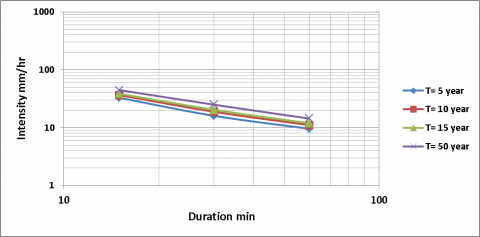
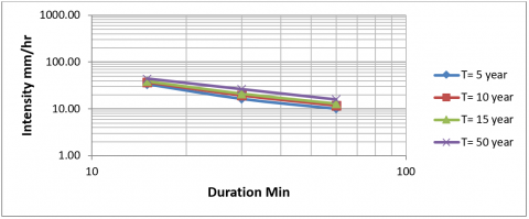
In Table 6, you can find the intensities calculated using the Gumbel distribution specifically for the Babylon station. Figure 3 presents the IDF curves for the Babylon station, which are utilized in this research for the Gumbel distribution.
Figure 3. IDF curve for Babylon station (Gumbel distribution)
4.3 Log normal distribution
In the Log Normal distribution, the frequency factor value is determined using a similar method as in the Normal distribution. However, when it comes to severe rainfall intensity, the value depends on the logarithm of the data. This value is then utilized in Eq. (7) to calculate the extreme rainfall intensity [21, 22]. As shown in Table 8 results for Babylon station (Log Normal distribution).
$y_t=\bar{y}+K_t S_y$ (7)
Table 8. Results for Babylon station (Log Normal distribution)
|
Duration (min) |
Intensity (mm/hr) |
|||
|
|
5 y |
10 y |
15 y |
50 y |
|
15 |
33.58 |
37.18 |
39.08 |
44.41 |
|
30 |
16.36 |
19.45 |
21.18 |
26.32 |
|
60 |
10.10 |
11.89 |
12.88 |
15.80 |
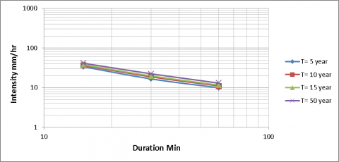
Figure 4. IDF curve for Babylon station (Normal distribution)
Figure 5. IDF curve for Babylon station (Log Normal distribution)
At the Babylon station in Iraq, IDF curves are created using three different statistical distributions: the Gumbel extreme value distribution, the Normal distribution, and the Log Normal distribution. The findings reveal that, when considering durations of 15, 30, and 60 minutes, Normal distribution proves to be more accurate and reliable compared to Gumbel and Log Normal distributions. As illustrated in Figures 4 and 5, Normal distribution was successful through the proximity of curve periods with each other, the quality of the fit tests between the three methods of distribution (gamma, normal and Log Normal) is to test Anderson-Darling as shown in Table 5, significant value (α) is equal (0.05) and degrees of freedom are equal (1). The constant value of the three distributions was less than the critical value, which means that the data tracked the distribution Anderson-Darling That is, we accept the false premise. On the other hand, we note that the test results from the distribution of gamma in the Moments method Lower than Normal and log Normal distributions, indicating that the distribution of gamma in the Moments method is the best. So "the three distributions (Normal and Log Normal and Gamma) are successful and suitable for test Chi-square and Kolmogorov-Smirnov and Anderson-Darling. The impact of IDF curves on the design, operation and maintenance of engineering infrastructure such as urban drainage systems, channels and bridges. In standard hydrological practice, IDF curves are developed by analysing rainfall data at observation points. Further studies are recommended when more information and data are available to verify the results obtained and update IDF curves.
This study employs three different probability distributions: Normal, Log Normal, and Gamma distributions to analyze rainfall data from a specific weather station in Babylon, Iraq. The parameters of these distributions are estimated using moments and maximum likelihood methods. To assess how well these theoretical distributions fit the actual data, three goodness of fit tests are conducted: Chi-square, Kolmogorov-Smirnov, and Anderson-Darling tests. The results of the Chi-square test indicate that the Normal distribution fits well for the Babylon station when both moments and maximum likelihood methods are applied. Similarly, the Log Normal distribution also fits well for Babylon station when estimated using both methods. The Gamma distribution also proves to be a good fit for the Babylon station when analyzed using moments and maximum likelihood methods.
Using Excel Software, the best results distribution was identified, with the Normal distribution standing out as the most fitting choice for the Babylon station data. The Normal distribution proved superior to the Gumbel and Log Normal distributions, boasting the lowest sum of differences between the period’s curves. Evaluation through the Kolmogorov-Smirnov index confirmed the suitability of Babylon station for all three distributions, assessed through both moments and maximum likelihood approaches.
Anderson-Darling test results showed that available data tracked the distribution of gamma in the moments method with significant value (0.05). However, the exact distribution between them cannot be determined. Further studies are recommended when More information and data are available to verify the results obtained and update IDF curves.
Table 9 shows the results of distributions and the best methods for each test.
Table 9. Best results for each test
|
Station |
Chi-square |
K – S |
A - D |
|||
|
distribution |
method |
dis. |
me |
dis. |
me |
|
|
Babylon |
Gamma |
M.L |
Gamma |
M. |
Gamma |
M. |
|
μ |
Mean |
|
σ |
Standard deviation |
|
f(x) |
Density function for a distribution |
|
x |
Independent variable |
|
y |
Independent variable for logarithm |
|
ꞵ, λ |
Gamma distribution parameters |
|
Г |
Gamma function |
|
$\chi^2$ |
Chi-square test |
|
Kt |
Frequency factor |
|
T |
Return period |
|
t |
Duration |
|
n |
The number of elements in the sample |
|
AD |
Anderson-Darling test |
[1] Omran, Z.A., Al-Bazzaz, S.T., Ruddock, F. (2014). Statistical analysis of rainfall records of some Iraqi meteorological stations. Journal of Babylon University Engineering Sciences, 22(1): 67-77.
[2] Miller, J., Taylor, C., Guichard, F., Peyrillé, P., Vischel, T., Fowe, T., Panthou, G., Visman, E., Bologo, M., Traore, K., Coulibaly, G., Chapelon, N., Beucher, F., Rowell, D.P., Parker, D.J. (2022). High-impact weather and urban flooding in the West African Sahel-A multidisciplinary case study of the 2009 event in Ouagadougou. Weather and Climate Extremes, 36: 100462. https://doi.org/10.1016/j.wace.2022.100462
[3] Gu, X., Ye, L., Xin, Q., Zhang, C., Zeng, F., Nerantzaki, S.D., Papalexiou, S.M. (2022). Extreme precipitation in China: A review on statistical methods and applications. Advances in Water Resources, 163: 104144. https://doi.org/10.1016/j.advwatres.2022.104144
[4] Reder, A., Raffa, M., Padulano, R., Rianna, G., Mercogliano, P. (2022). Characterizing extreme values of precipitation at very high resolution: An experiment over twenty European cities. Weather and Climate Extremes, 35: 100407. https://doi.org/10.1016/j.wace.2022.100407
[5] Ouarda, T.B., Yousef, L.A., Charron, C. (2019). Non‐stationary intensity‐duration‐frequency curves integrating information concerning teleconnections and climate change. International Journal of Climatology, 39(4): 2306-2323. https://doi.org/10.1002/joc.5953
[6] Campos, J.N.B., Studart, T.M.D.C., Souza Filho, F.D.A.D., Porto, V.C. (2020). On the rainfall intensity-duration-frequency curves, partial-area effect and the rational method: Theory and the engineering practice. Water, 12(10): 2730. https://doi.org/10.3390/w12102730
[7] Silva, D.F., Simonovic, S.P., Schardong, A., Goldenfum, J.A. (2021). Assessment of non-stationary IDF curves under a changing climate: Case study of different climatic zones in Canada. Journal of Hydrology: Regional Studies, 36: 100870. https://doi.org/10.1016/j.ejrh.2021.100870
[8] Bezak, N., Šraj, M., Mikoš, M. (2016). Copula-based IDF curves and empirical rainfall thresholds for flash floods and rainfall-induced landslides. Journal of Hydrology, 541: 272-284. https://doi.org/10.1016/j.jhydrol.2016.02.058
[9] U.S. Army Corps of Engineers. (1994). Engineering and design Flood-Runoff analysis. Department of the Army, Engineer Manual 1110-2-1417, Washington, DC 20314-1000.
[10] Schlef, K.E., Kunkel, K.E., Brown, C., Demissie, Y., Lettenmaier, D.P., Wagner, A., Wigmosta, M.S., Karl, T.R., Easterling, D.R., Wang, K.J., et al. (2022). Incorporating non-stationarity from climate change into rainfall frequency and intensity-duration-frequency (IDF) curves. Journal of Hydrology, 616: 128757. https://doi.org/10.1016/j.jhydrol.2022.128757
[11] Montgomery, D.C. (2003). Applied Statistics and Probability for Engineers. John Wiley & Sons, Inc.
[12] Vose, D. (2010). Fitting distributions to data and why you are probably doing it wrong. http://www.vosesoftware.com.
[13] Reich, B.M., Osborn, H.B. (1982). Improving point rainfall prediction with experimental watershed data. In Proceedings of the International Symposium on Rainfall-Runoff Modeling, Tucson, Arizona.
[14] Jäntschi, L., Bolboacă, S.D. (2018). Computation of probability associated with Anderson-Darling statistic. Mathematics, 6(6): 88. https://doi.org/10.3390/math6060088
[15] Saf, B. (2005). Evaluation of the synthetic annual maximum storms. Pamukkale University, Denizli, Turkey. The Electronic Journal of the International Association for Environmental Hydrology, vol. 13.
[16] Erto, P., Lepore, A. (2011). A note on the plotting position controversy and a new distribution-free formula. Intervento Presentato al Convegno 45th Scientific Meeting of the Italian Statistical Society. CLEUP, pp. 1-7.
[17] Krishnamoorthy, K. (2006). Handbook of statistical distributions with applications. Chapman and Hall/CRC. University of Louisiana at Lafayette, U.S.A. https://doi.org/10.1201/9781420011371
[18] Prodanovic, P., Simonovic, S.P. (2007). Development of rainfall intensity duration frequency curves for the City of London under the changing climate. Department of Civil and Environmental Engineering, The University of Western Ontario. London, Ontario, Canada.
[19] Ginos, B.F. (2009). Parameter Estimation for the Lognormal Distribution. Brigham Young University.
[20] Yüksek, Ö., Anılan, T., Saka, F., Orgun, E. (2022). Rainfall intensity-duration-frequency analysis in Turkey, with the emphasis of eastern black sea basin. Teknik Dergi, 33(4): 12087-12103. https://doi.org/10.18400/tekderg.727085
[21] Ginos, B.F. (2009). Parameter Estimation for the Lognormal Distribution. Brigham Young University.
[22] Tran, T.S., Xuan, A.H. (2023). Deriving of intensity–duration–frequency (IDF) curves for precipitation at Hanoi, Vietnam. E3S Web of Conferences, 403: 06002. https://doi.org/10.1051/e3sconf/202340306002