Dahir Mohamed Ali![]()
© 2024 The author. This article is published by IIETA and is licensed under the CC BY 4.0 license (http://creativecommons.org/licenses/by/4.0/).
OPEN ACCESS
This study investigated the environmental sustainability of economic growth: a Panel data analysis in East Africa for the period 1990-2020 And we use of OLS estimation, Fully Modified Least Squares (FMOLS), and the outcome of Descriptive statistics reveal the typical magnitudes, standard deviations, and ranges of variables such as ecological footprint (EF), carbon dioxide (CO2), biocapacity (BC), foreign direct investment (FDI), gross domestic product (GDP), and population. EF has an average of 17.15 with a low standard deviation, suggesting proximity to the mean. CO2 exhibits higher variability, with a range from -3.330 to 11.691. Similar patterns are observed for BC, FDI, GDP, and population. Correlation analysis reveals relationships, with positive correlations between EF and CO2, EF and population, CO2 and population, and BC and EF. Negative correlations exist between EF and GDP and CO2 and GDP, suggesting potential trends in the associations between ecological impact, economic development, and population dynamics. The Kao Residual Cointegration Test indicates that the variables in the analysis may be stationary after differencing, a crucial condition for cointegration. The p-values associated with residual V and HAC V are both less than 0.05, providing statistical significance and evidence against the null hypothesis of no cointegration. The overall low p-value (0.0004) for the Kao test further supports the rejection of the null hypothesis, suggesting the presence of cointegration among the variables. For biocapacity (BC) and foreign direct investment (FDI), individual intercept and trend co-integration tests show significant evidence.
economic growth, biodiversity conservation, environmental sustainability, ecosystem services, climate change adaptation, carbon-dioxide
In the dynamic landscape of East Africa, the intersection between environmental sustainability and economic growth stands as a pivotal nexus that warrants meticulous investigation. As nations in the region strive for prosperity, they grapple with the intricate challenge of fostering robust economic development while concurrently safeguarding their fragile ecosystems. Environmental boundaries range from local to global, according to ecological economics. It covers everything from long-term ideas of sustainable societies to short-term policy and local crisis research. Environmental economics also considers global issues, including carbon emissions, deforestation, overfishing, and the loss of species [1]. This study embarks on a comprehensive exploration of the intricate relationship between environmental sustainability and economic growth in East Africa, employing the sophisticated lens of Panel Data Analysis. By delving into the empirical nuances of this dynamic interaction, we aim to shed light on the critical interplay between human activities and the environment, providing actionable insights for policymakers, practitioners, and stakeholders invested in the sustainable future of the region. One of the most important aspects of environmental sustainability is its forward-looking orientation because so many decisions that influence the environment are not recognized right away. environmental protection sector, and increasing public knowledge of environmental protection [2]. With its exceptional biodiversity, East Africa presents a distinct mix of opportunities and challenges for sustainable development. Nuanced care is required to strike a delicate balance between protecting the region's ecological integrity and utilizing its natural resources for economic prosperity. Therefore, it is improbable that developing countries will exactly mimic the environmental histories of rich ones [3].
1.1 Research questions
What is the Nature and extent of the relationship between environmental sustainability and economic growth in East Africa over the specified period?
Subsidiary research questions
How have key environmental indicators (e.g., Ecological Footprint carbon emissions, and biocapacity) advanced in East Africa during the study period?
What are the forms and trends in economic growth indicators (e.g., GDP per capita, Population rate, and investment patterns) across East African countries?
1.2 Hypothesis
Null hypothesis (H0):
There is no significant relationship between environmental sustainability indicators and economic growth indicators in East Africa.
Alternative Hypothesis (H1):
There exists a significant and positive relationship between environmental sustainability indicators and economic growth indicators in East Africa.
Specific Hypothesis:
H1a: Higher levels of environmental sustainability, as measured by reduced carbon emissions and conservation efforts, are associated with higher economic growth rates in East African countries. H1b: Effective policy interventions focused on environmental sustainability contribute positively to economic growth in the region.
Temporal Hypothesis:
H2: Over the study period, improvements in environmental sustainability precede or coincide with subsequent positive changes in economic growth indicators.
Spatial Hypothesis:
H3: There are spatial dependencies in the relationship between environmental sustainability and economic growth, with neighboring countries exhibiting similar trends due to shared environmental and economic characteristics.
This study makes a noteworthy contribution to the existing literature on ecological economics in East Africa by filling in important knowledge gaps, presenting actual data, and providing sophisticated insights into the interplay between economic growth and environmental sustainability. The following are some ways that this work advances the field: Although ecological economics is a well-established discipline, there is not much research that concentrates on East Africa in particular. The empirical data presented in this study is region-specific and captures the distinct possibilities and problems that East African countries confront in striking a balance between environmental sustainability and economic growth. this study's results aim to provide useful and policy-relevant information. Policymakers can promote sustainable development by determining the precise mechanisms and factors that affect the link between environmental sustainability and economic growth in East Africa.
The study's incorporation of temporal and geographical assumptions gives ecological economics research in East Africa a fresh perspective. The study provides a more thorough knowledge of the contextual elements influencing the link between environmental sustainability and economic growth by looking at how these dynamics play out over time and location. this study makes a valuable contribution to the field of ecological economics in East Africa by providing empirical evidence, employing advanced analytical methods, offering policy insights, and addressing specific regional challenges. By doing so, it enriches the existing body of knowledge and lays the groundwork for more targeted and effective interventions in the pursuit of sustainable development in the East African context.
The theoretical framework exploring the relationship between environmental sustainability and economic growth encompasses several prominent perspectives.
2.1 Environmental Kuznets curve
Early in the 1990s, the North American Free Trade Agreement (NAFTA) impact research by Grossman and Krueger and the background study for the 1992 World Development Report by Shafik and Bandyopadhyay led to the development of the EKC idea. However, a key component of the sustainable development argument put forth by the World Commission on Environment and Development in Our Common Future is that economic growth is required to preserve or improve environmental quality [4]. The Environmental Kuznets Curve idea has been tested in many studies in the literature. In general, these studies use cubic and quadratic models. The relationship between GDP and CO2 emissions is investigated using quadratic models to determine whether it follows a U-shaped or an inverted U-shaped curve. Contrarily, cubic models investigate whether a curve with an N-shape or an inverted N-shape arises when variables are related.
In addition, the literature suggests including other variables in the analysis in addition to the quadratic or cubic models. Many of the previous studies that looked at it found that the Environmental Kuznets Curve theory is accurate for Turkey. The research investigated the EKC hypothesis as well as the pollution haven hypothesis (PHH) in Turkey over the period of 1970-2016 by integrating foreign direct investments, renewable energy consumption, and industrialization variables into the quadratic model using the ARDL approach. Investigations on the causal links between sustainability indices and economic growth also focus on policy-relevant methods [5]. The primary objective of the article is to make human progress sustainable for both present and future generations while fostering harmony with the rest of the biosphere. To this end, the ecological footprint is examined as a tool for constructing biophysically-based ecological economics [6]. China's social and economic progress depends on urbanization, yet resource scarcity and pollution are obstacles. The huge pollution burden in Beijing, the capital, necessitates a decoupling between economic expansion and environmental degradation. The Environmental Kuznets Curves (EKC) study reveals that while emissions are still high, pollution intensity hit a turning point around 2006. Adjustments to industrial structure, urban planning, pollution control measures, and technological improvements are among the factors causing this shift. Beijing and the surrounding areas have worked together to reduce air pollution [7].
2.2 Relationship between environmental sustainability and economic development
The connection between environmental pressure and economic development is a topic of ongoing controversy. While some theories link environmental deterioration (ED) to economic growth, others promote economic development for better environmental quality and sustainability. They contend that when consumption and production increase, atmospheric pressure and air pollution do as well. They do, however, support the idea that high-income nations are better able to balance pollution and consumption than low-income nations. The amount of pressure on the environment is also impacted by energy. Use the literature like [8] among others, supports the ED. Most nations have prioritized economic development over environmental concerns, which has resulted in water and air pollution, pesticides in food, a decreasing ozone layer, and rising global temperatures.
This study is aimed at testing empirically the economic development hypothesis introduced by Simon Kuznets in 1966: that during economic development, income disparities rise in the beginning and then begin to fall. This has been represented in an inverted U-shape relationship known as the Kuznets curve. This study hypothesizes a Kuznets-type relationship between the rate of environmental degradation and the level of economic development. The hypothesis is tested using cross-sectional data on deforestation and air pollution from a sample of developing and developed countries. After confirming the reality of the Kuznets curve, the implications for policy formulation are then derived for the areas of employment, technology transfer, and development assistance.
The focus of this study is on China and India's environmental Kuznets curves and how they affect the quality of the environment worldwide. Environmental Kuznets curves at the individual and panel levels are identified using data from 1972 to 2017. The findings indicate that while India's environmental quality will improve with an increase in per capita GDP after the threshold level, China's quality will deteriorate at a slower rate due to high energy use. Although the analysis aids in formalizing the relationship between the two Asian economies, it is unable to predict when they will gain from the Kuznets curve's downward trend [9].
2.3 The linkage between ecological footprint and economic growth
The significance of China and India's choices for global sustainability is highlighted in the report. Over the past 45 years, China's per capita ecological footprint has rapidly increased despite the country's middle-income status, whereas India's footprint has somewhat dropped [10]. With a focus on Nigeria's contribution to international efforts to combat global warming, the report analyzes Nigeria's economic performance and ecological imprint. The study also demonstrates a favorable association between independent factors such as energy use, agriculture, FDI, and ecological impact. The causation test indicates a one-way transmission from population expansion, energy use, and ecological imprint to economic growth. The results imply that growth-based emissions in Nigeria require a well-structured policy to address them [11]. Due to its complicated relationship to economic growth, biodiversity, ecosystem services, and human well-being, the ecological footprint—a measure of environmental degradation—is frequently disregarded in political decision-making. This study demonstrates how economic expansion increases the ecological footprint while biocapacity also contributes to environmental degradation using the autoregressive distributive lag econometric approach [12].
2.4 The relationship between ecological footprint and FDI
The study focuses on how foreign direct investment (FDI) affects the pace of physical bioprotective land exhaustion. It compares the ecological performance of industrialized and emerging nations as well as "clean" and "dirty" sectors. The paper examines the ecological impacts of six sector-level FDI flows using a dynamic panel model with an environmental Kuznets curve. Results reveal that although low- and middle-income nations suffer an ecological impact related to production, high-income countries experience an ecological impact related to consumption. FDI in financial services lowers EF in high-income nations [13].
The study explores how FDI has affected the economic development of Somalia. DFDI does not significantly affect GDP at the 5% level, but it does considerably affect GDP at the 0.005 level, according to a VAR model analysis. Wald tests for Granger causality reveal that FDI is independent [14]. Advanced clean technology should be promoted in FDI manufacturing areas by regulations on production processes [15].
Econometric Approach: To analyze the impact of environmental sustainability on economic development, we employ a Panel Data Analysis approach. This method allows us to account for time series panel data and, offers a more robust analysis of the dynamic relationship between the variables. Panel data structure to account for country-specific heterogeneity and capture unobserved factors that might impact the association, fixed-effects models are used in the panel, which is composed of a balanced dataset containing observations for each East African nation throughout many periods. Our econometric model is designed to estimate the causal relationship between environmental sustainability indicators and economic development metrics. Key independent variables include carbon emissions, population, FDI, and GDP per capita. Dependent variables consist of ecological footprint and six sub-groups. This method section provides openness and clarity on how the study explores the intricate link between environmental sustainability and economic growth in the East African setting by outlining the data sources, econometric technique, and validation processes (Tables 1 and 2).
Table 1. Ecological foot printing
|
Ecological Footprint |
Biocapacity |
|
Cropland |
Cropland |
|
Grazing land |
Grazing land |
|
Fishing grounds |
Fishing grounds |
|
Forest |
Forest |
|
Built-up land |
Built-up land |
|
Carbon land |
NA |
|
Major land types used in biocapacity and ecological footprint accounting. Forest land ecology represents the biocapacity related to carbon dioxide emissions National Footprint Accounts, 2020 edition, by Global Footprint Network. accessible at https://www.footprintnetwork.org/our-work/ecological-footprint/ |
|
3.1 Data sources
Table 2. Sources of data and variables
|
Variables |
Abbreviations |
Sources |
|
Ecological footprint |
EF |
World Bank Global Footprint Network |
|
Carbon-diode |
CO2 |
|
|
Population |
Poup |
|
|
Foreign direct investment |
FDI |
|
|
Biocapacity |
BC |
3.1.1 Data limitations
Availability and Consistency The analysis uses data gathered from several sources, including environmental databases like Global Footprint Network and the World Bank. Data consistency and availability can change over time and between nations, which might lead to biases or measurement inaccuracies. Data gaps Challenges may arise from missing or incomplete data on specific economic measurements, environmental indicators, or policy factors. Imputing missing numbers might result in the introduction of new uncertainties, which would affect the accuracy.
This study examines the effects of environmental sustainability on economic development in ten samples of East African nations: Kenya, Malawi, Mozambique, and Rwanda. Uganda, Zambia, and Zimbabwe Somalia, Comoros, Ethiopia, Mauritius, Sudan, and Madagascar Data sources include some variables such as GDP, FDI, POPU, and CO2 from World Bank indicators (WBD) from 1990 to 2020 and others such as EF and BC, and all six sub-groups such as built-up land, cropped land, carbon land, grazing land, fishing grounds, and forests came from Global Footprint Network Data. The ecological footprint and biocapacity statistics from the Global Footprint Network (2020) database, the amount of carbon dioxide produced per person, the gross domestic product, and foreign direct investment to perform ordinary least squares (OLS) were all observed in this study as dependent and independent factors. The models used in the study were developed by those used by Bagliani et al. [16].
$\mathrm{EF}=\beta_0+\beta_1 \mathrm{GDP}_{\mathrm{it}}+\beta_2(G D P)_{i t}{ }^2+\beta_2 \mathrm{CO} 2_{\mathrm{it}}\begin{aligned} & +\beta_3 \mathrm{BC}_{\mathrm{it}}+\beta_4 \mathrm{FDI}_{\mathrm{it}}+\beta_5 \mathrm{POPU}_{\mathrm{it}} +\varepsilon_{\mathrm{it}}\end{aligned}$ (1)
where, ' $\beta_0$ ' is the intercept and ' $\varepsilon_{\mathrm{it}}$ ' is residual. The subscript ' $\mathrm{i}$ ' refers to the cross-sectional dimension across the state, and ' $\mathrm{t}$ ' represents the time dimension (i.e., $\mathrm{t}=1990$, 2020).
The extended model is as follows:
$\begin{aligned} E F=\beta_0+\beta_1 G D & P_{i t}+\beta_2(G D P)_{i t}{ }^2+\beta_3 C O 2_{i t} +\beta_4 B C_{i t}+\beta_5 F D I_{i t} +\beta_5 P O P U_{i t}+\varepsilon_{i t}\end{aligned}$ (2)
where, GDP per capita2 refers to the quadratic term of GDP per capita and shape EKC curve. To study the Ecological Footprint per capita of six groups of land, this is the equation form:
$\begin{aligned} y_{i t}=\beta_0+\beta_1 G D & P_{i t}+\beta_2(G D P)_{i t}{ }^2+\beta_3 C O 2_{i t} +\beta_4 B C_{i t}+\beta_5 F D I_{i t}+\beta_5 P O P U_{i t} +\varepsilon_{i t}\end{aligned}$ (3)
where, yit stands for all the EF per capita subgroups in the 'i' country now, including buildup land, carbon-absorbing land, farmland, fishing grounds, forest products, and grazing land.
This justification places a strong emphasis on the region's variety, the value of representative sampling, and the necessity of taking environmental, economic, and policy considerations into account when choosing which nations to include in the panel data analysis.
4.1 Fully modified OLS (FMOLS)
We use OLS (Ordinary Least Squares), FMOLS (Fully Modified Ordinary Least Squares), and panel cointegration analysis in the context of your study on "Environmental Sustainability and Economic Growth: A Panel Data Analysis in East Africa.
Under certain circumstances, OLS, a common regression technique, yields unbiased coefficient estimates. Within the framework of our research, ordinary least squares (OLS) constitute the standard approach for analyzing the connection between environmental sustainability measures and economic development metrics at the national level. When evaluating panel time series data, OLS is very helpful as it can reveal preliminary patterns and trends in the connection between the variables. With its help, we can calculate the average impact of environmental sustainability on economic growth across all East Africa.
An expansion of OLS that deals with possible endogeneity and cointegration problems is called FMOLS. Given that shared long-term trends are expected to have an impact on both environmental sustainability and economic growth, FMOLS offers a more reliable framework for evaluating the link while taking potential biases into account. We can account for endogeneity issues and any misleading correlations using FMOLS since the link between environmental sustainability and economic growth is dynamic and multifaceted. This method is very useful for examining whether there are any long-term correlations in the data.
Study as dependent and independent factors. Model used in the study were developed by those used by Bagliani et al. [16], Ansari et al. [17], and Majeed and Mazhar [18]. The panel cointegration models are used to explore issues related to long-run economic linkages that are frequently seen in macroeconomic and financial data. Economic theory frequently predicts such a long-term relationship, making it crucial to estimate the regression coefficients and determine whether they adhere to theoretical requirements.
The asymptotic features and statistical tests of panel cointegrated regression models and time series cointegrated regression models differ, according to recent studies [19-21].
4.2 Unit root test
A range of tests for unit roots, also known as stationarity, in panel datasets, are carried out using xtunitroot. The null and alternative hypotheses are stated explicitly at the top of each test's result [22]. Two generations of tests—the first generation (Levin, Lin, and Chu test, 2002; Pesaran, and Shin test, 2003) whose main limit is the of the average long-run covariances, ₳, and Ώ, we may describe the adapted DV and serial connection improvement terms.
$\begin{gathered}\mathrm{y}_{\mathrm{it}}{ }^{\mp}=\mathrm{y}_{\mathrm{it}}^{-}-\omega_{12} \Omega_{22}^{-1} \overline{\mathrm{u}}_2 \text { and } \lambda_{12}^{+}=\lambda_{12}-\omega_{12} \Omega_{22}^{-1} \mathcal{A}_{22}\end{gathered}$ (4)
$\widehat{\beta} E F=\left\{\Sigma_{i-1}^N \Sigma_{t-1}^N\left(\mathrm{x}_{\mathrm{it}}-\overline{\mathrm{x}}_{\mathrm{t}}\right)\right\}^{-1}\left\{\Sigma_{\mathrm{i}-1}^{\mathrm{N}}\left(\Sigma_{\mathrm{t}-1}^{\mathrm{N}}\left(\mathrm{x}_{\mathrm{it}}-\overline{\mathrm{x}}_{\mathrm{t}}\right) \hat{\mathrm{y}}_{\mathrm{it}}^{+}-\mathrm{T} \hat{\Delta}_{\varepsilon \mathrm{u}}^{+}\right)\right\}$ (5)
Above Eq. (5) of FMOLS indicates the measurement of the cross segment by $\mathrm{N}$, period by $\mathrm{T}$, and individual exact mean by $\bar{x}$. Nevertheless, $\hat{y}_{i t}^{+}$ and $\hat{\Delta}_{\varepsilon u}^{+}$ demonstrating endogeneity sequence modification and correction period. assumption of cross-sectional independence across units, and the second generation of tests that rejects the cross-sectional independence hypothesis - have been developed within the panel unit root test framework [23]. Typically, imitation of restrictive supplies defined as functionals of Brownian movements is used to determine critical standards for unit root testing [24].
4.3 Panel cointegration analysis
Panel cointegration analysis is essential for examining the long-term relationships between variables in a panel dataset. This technique helps to identify whether environmental sustainability indicators and economic development metrics move together over time, indicating a stable and sustainable relationship. Environmental and economic variables often exhibit persistent trends that can be better captured through cointegration analysis. In the context of East African countries, where long-term environmental policies may influence economic outcomes, panel cointegration analysis allows us to explore the presence of a stable equilibrium in the relationship.
Pedroni's [19] parametric group-t, panel-rho, group-rho, parametric panel-t, and Larsson's standardized LR-bar statistic are all taken into consideration in the work of McCoskey and Kao [25]. The first-generation panel cointegration tests, which presume cross-sectional independence while testing for cointegration, were the foundation for the EKC literature prior to the 2010s, much like the panel unit root tests [26].
This long-run equilibrium is evaluated and quantified in statistics and econometrics using the cointegration concept. When two or more time series are nonstationary, cointegration takes place. possess a long-term balance. So that their linear combination yields a stationary time series, they should move in tandem. possess the same stochastic trend at the foundation.
In this part the empirical findings provide concrete evidence regarding the dynamics between environmental sustainability and economic growth. these findings contribute to the ongoing discourse surrounding the feasibility of achieving sustainable development goals and offer insights into the nuanced interplay between economic activities and environmental well-being.
Both the above-mentioned tables display the unit root test at level and first and second differencing. Table 3 shows that the variables, such as ecological footnote per capital (EF), carbon dioxide (CO2), and biocapacity (BC) per capital, FDI, and population, are statistically insignificant at the level of significance because the p-value is less than 5%, which refers to the acceptance of null hypotheses. That means all the variables are nonstationary at level.
On the other hand, Table 4 shows that the variables, such as ecological footnote per capital (EF), carbon dioxide (CO2), and biocapacity (BC) per capital, FDI, and population, are statistically significant at first differencing because the p-value is less than 5% level of significance, which refers to the rejection of null hypotheses. That means all the variables are stationary at first differencing.
Table 3. Unit root checking for variables at level
|
Individual Intercept |
||||||||||||
|
|
T-Test |
EF |
T-Test |
LCO2 |
T-Test |
LBC |
T-test |
LFDI |
T-test |
LGDP |
T-Test |
LPopu |
|
|
|
P -V |
|
P -V |
|
P-V |
|
P -V |
|
P -V |
|
P -V |
|
LLC |
-1.72 |
0.042 |
-2.40 |
0.008 |
-0.06 |
0.47 |
-8.89 |
0.000 |
-6.88 |
0.000 |
-3.45 |
0.00 |
|
IPS |
2.063 |
0.980 |
-0.19 |
0.424 |
2.031 |
0.97 |
-8.66 |
0.000 |
-1.76 |
0.038 |
4.13 |
1.00 |
|
ADF |
18.76 |
0.846 |
32.2 |
0.184 |
16.64 |
0.91 |
72.5 |
0.000 |
52.84 |
0.00 |
13.7 |
0.97 |
|
PP |
27.73 |
0.371 |
22.06 |
0.685 |
27.47 |
0.38 |
143.8 |
0.000 |
46.90 |
0.007 |
28.6 |
0.32 |
|
Individual Intercept and Trend |
||||||||||||
|
LLC |
-0.84 |
0.19 |
-2.83 |
0.002 |
0.365 |
0.64 |
-11.4 |
0.000 |
2.567 |
0.994 |
-5.740 |
0.000 |
|
BRT |
-0.84 |
0.19 |
1.04 |
0.851 |
-1.85 |
0.03 |
-1.67 |
0.047 |
2.576 |
0.995 |
2.758 |
0.997 |
|
IPS |
-0.73 |
0.23 |
0.28 |
0.611 |
-3.02 |
0.00 |
-8.41 |
0.000 |
-1.479 |
0.069 |
-4.539 |
0.000 |
|
ADF |
49.8 |
0.00 |
35.2 |
0.105 |
53.33 |
0.00 |
322.1 |
0.000 |
62.57 |
0.001 |
75.38 |
0.000 |
|
PP |
46.17 |
0.00 |
19.3 |
0.820 |
97.13 |
0.00 |
151.4 |
0.000 |
311.9 |
0.000 |
80.76 |
0.000 |
Author’s Source: WBD, E-views
Table 4. Unit root checking for variables in first differencing
|
Individual Intercept |
||||||||||||
|
|
T-Test |
EF |
T-Test |
LCO2 |
T-Test |
LBC |
T-Test |
LFDI |
T-Test |
LGDP |
T-Test |
LPopu |
|
|
|
P -V |
|
P -V |
|
P-V |
|
P -V |
|
P -V |
|
P -V |
|
LLC |
-9.21 |
0.000 |
-6.15 |
0.000 |
-14.1 |
0.00 |
-11.7 |
0.000 |
10.58 |
1.000 |
-6.005 |
0.000 |
|
IPS |
-12.6 |
0.000 |
-9.74 |
0.000 |
-18.2 |
0.00 |
-17.1 |
0.000 |
-5.677 |
0.000 |
-10.42 |
0.000 |
|
ADF |
186.1 |
0.000 |
140.9 |
0.000 |
262.4 |
0.00 |
257.2 |
0.000 |
81.78 |
0.000 |
141.9 |
0.000 |
|
PP |
326.1 |
0.000 |
253.3 |
0.000 |
367.5 |
0.00 |
282.7 |
0.000 |
171.1 |
0.000 |
90.71 |
0.000 |
|
Individual Intercept and Trend |
||||||||||||
|
LLC |
-7.01 |
0.000 |
-5.66 |
0.000 |
-11.2 |
0.00 |
-10.0 |
0.000 |
18.49 |
1.000 |
-7.193 |
0.000 |
|
BRT |
-9.65 |
0.000 |
-3.38 |
0.000 |
-7.73 |
0.00 |
-4.90 |
0.000 |
2.431 |
0.992 |
-0.699 |
0.242 |
|
IPS |
-11.6 |
0.000 |
-8.65 |
0.000 |
-17.0 |
0.00 |
-15.7 |
0.000 |
-3.23 |
0.000 |
-10.97 |
0.000 |
|
ADF |
165.8 |
0.000 |
117.5 |
0.000 |
294.7 |
0.00 |
239.2 |
0.000 |
58.35 |
0.000 |
380.7 |
0.000 |
|
PP |
783.9 |
0.000 |
517.6 |
0.000 |
616.6 |
0.00 |
1946. |
0.000 |
382.5 |
0.000 |
308.2 |
0.000 |
Author’s Source: WBD, E-views
5.1 Descriptive analysis and correlation
The procedure of descriptive analysis entails examining and summarizing a dataset's salient attributes. It seeks to give a succinct and understandable summary of the key features of the data, assisting in the identification of its distribution, variability, and central patterns. In this kind of study, graphical representations and descriptive statistics are frequently employed. A correlation matrix is a table that shows the correlation coefficients between many variables. Each cell in the table represents the correlation between two variables, and the diagonal of the matrix typically shows the correlation of each variable with itself (which is always 1).
Table 5. Descriptive analysis
|
Variable |
Obs. |
Mean |
Std.Dev. |
Min |
Max |
|
Ecological Footprint |
398 |
17.150 |
1.0185 |
15.254 |
19.131 |
|
LCO2 |
398 |
0.5020 |
4.2291 |
-3.220 |
11.691 |
|
L Biocapacity |
398 |
16.682 |
1.5913 |
11.871 |
18.426 |
|
LFDI |
398 |
0.2053 |
1.587 |
-8.927 |
3.695 |
|
LGDP |
398 |
10.334 |
4.069 |
-1.026 |
16.052 |
|
L Population |
398 |
16.986 |
0.8242 |
15.553 |
19.130 |
Author’s Source: WBD, E-views
Table 5 shows that the "L Ecological footprint" variable in a dataset has an average of 17.15, indicating a typical magnitude of ecological footprints. The low standard deviation of 1.0185 suggests that the values of the ecological footprint are relatively close to the mean. The range from 15.25 to 19.131 measures variation, allowing researchers to identify values, spread, and understand diversity. These descriptive statistics are crucial for informed decision-making in environmental research and policy planning. The "LCO2" variable, with a mean of 0.50, provides an average carbon dioxide level in the dataset.
However, the relatively higher standard deviation of 4.229 indicates greater variability, suggesting that carbon dioxide levels are more dispersed from the mean. Which indicates a range of values from -3.330 to 11.691. Analyzing this range helps identify the spread of carbon dioxide values and provides insights into the diversity of carbon dioxide levels within the dataset. The "L Biocapacity" variable in a dataset has an average of 16.682, indicating a typical magnitude of biocapacity. The low standard deviation of 1.5913 suggests that the values of the biocapacity are relatively close to the mean. The range from 11.871 to 18.426 measures variation, allowing researchers to identify values, spread, and understand diversity.
On the other hand, the "LFDI" variable in the dataset gives an average of foreign direct investment with a mean of 0.20. The comparatively higher standard deviation of 1.587, however, points to more variability and suggests that the levels of foreign direct investment are more widely distributed than the norm. It shows a range of values between 3.695 and -8.927. This range's analysis sheds light on the dataset's diversity of foreign direct investment levels as well as the distribution of foreign direct investment values.
The "L GDP" variable in a dataset has an average of 10.334, indicating a typical magnitude of gross domestic product. The low standard deviation of 4.069 suggests that the values of the gross domestic product are relatively close to the mean. The range from -1.026 to 16.052 measures variation, allowing researchers to identify values and understand diversity. On the other hand, "population.", The average population is 16.986, with a relatively lower standard deviation of approximately 0.8242. The mean range is from 15.553 to 19.130.
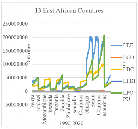
In summary, Figure 1 provides valuable insights into the diversity of responses among 13 East African countries regarding the impact of environmental sustainability and economic development, particularly focusing on the ecological footprint. The observed variability indicates a complex landscape that requires nuanced policy considerations for fostering sustainable practices in the region.
Figure 1. Diversity of responses among 13 East African countries
5.2 Correlation matrix
Table 6. Correlation analysis
|
LEF |
LCO2 |
LGDP |
LBC |
LFDI |
LPopu |
|
|
LEF |
1 |
|||||
|
LCO2 |
0.4386 |
1 |
||||
|
LGDP |
-0.215 |
-0.127 |
1 |
|||
|
LBC |
0.844 |
0.590 |
-0.31 |
1 |
||
|
LFDI |
-0.163 |
-0.067 |
0.101 |
-0.000 |
1 |
|
|
LPopu |
0.794 |
0.819 |
-0.173 |
0.836 |
-0.11 |
1 |
Table 6 shows the dependent variable (ecological footprint). Positive correlation with LCO2 (0.4386) and LPopu (0.794): As the ecological footprint increases, there is a moderately positive correlation with both carbon dioxide levels (LCO2) and population size (LPopu). Negative correlation with LGDP (-0.215): There is a weak negative correlation with gross domestic product (LGDP), suggesting a slight inverse relationship between ecological footprint and economic development.
On the other hand, LCO2 (carbon dioxide levels) Positive correlation with LEF (0.4386) and LPopu (0.819): Carbon dioxide levels have a moderately positive correlation with both ecological footprint and population size. Weak negative correlation with LGDP (-0.127): carbon dioxide levels show a slight negative correlation with gross domestic product. LGDP and other variables Weak negative correlation with LEF (-0.215): GDP and ecological footprint have a slight negative correlation, indicating a potential trend where economic development is associated with a lower ecological footprint. There was no strong correlation with LCO2 (0.127), LBC (-0.310), LFDI (0.101), or LPopu (-0.173). LBC (log biocapacity) and other variables Strong positive correlation with LEF (0.844): There is a strong positive correlation between biocapacity and ecological footprint, suggesting that regions with higher biocapacity tend to have a higher ecological footprint. Moderate positive correlation with LCO2 (0.590) and LPopu (0.836): Biocapacity has moderately positive correlations with both carbon dioxide levels and population.
LFDI and other variables, Weak negative correlation with LFDI (-0.163): Foreign direct investment shows a weak negative correlation with ecological footprint. There was no strong correlation with LCO2 (-0.067), LGDP (0.101), LBC (-0.000), and LPopu (-0.110). population Strong positive correlation with LEF (0.794) and LCO2 (0.819): Population size has strong positive correlations with both ecological footprint and carbon dioxide levels. Weak negative correlation with LGDP (-0.173): Population size has a weak negative correlation with gross domestic product.
5.3 Panel cointegration
To fully modify an ordinary square, we must use the specified dependent and independent variables. So, after we run the panel for Peter Pretonic, we can have three, as we mentioned: pterionic, cow, and fisher. For each one, we must use three types of methods: individual tests, individual intercepts, and no intercept.
Table 7 illustrations that Kao Residual Cointegration Test the test statistic is -3.343, and this is the negative The ADF test statistic suggests that the variables may be stationary after differencing, a crucial condition for cointegration analysis. The p-values associated with residual V and HAC V are both less than 0.05, indicating statistical significance. This provides evidence against the null hypothesis of no cointegration. The low overall p-value (0.0004) for the Kao Residual Cointegration Test further supports the rejection of the null hypothesis, indicating the presence of cointegration among the variables.
Table 7. Kao residual cointegration test
|
DV and IDV |
Ho Cio |
ADF |
Residua V |
HAC V |
|
|
|
-3.343 |
0.002939 |
0.001553 |
|
LEF |
|
|||
|
LBC |
|
|||
|
GDP, LCO2 LFDI, LPop |
P-value 0.0004 |
|||
This Table 8 appears to present the outcomes of the Pedroni panel cointegration test for different specifications, with and without individual intercepts and trends. Panel cointegration test result Ho says that there is no cointegration among the variables. Rejecting this hypothesis implies evidence of cointegration, indicating a long-term relationship among the specified variables.
Table 8. The outcome of the Pedroni panel cointegration
|
|
Co-Integration Test Ho Hypothesis: No Co-Integration |
Individual Intercept |
|
|
Statistic |
Weighted Statistic |
||
|
BC FDI GDP CO2 LPo |
Panel v-Statistic |
-2.314*** |
-2.653** |
|
Panel rho-Statistic |
-3.3028** |
-1.657 |
|
|
Panel pp-Statistic |
-6.46*** |
-7.863*** |
|
|
Panel ADF-Statistic |
-6.135** |
-2.66*** |
|
|
|
Group Rho -Statistic |
0.0544 |
|
|
Group PP -Statistic |
-8.139*** |
||
|
Group ADF -Statistic |
-3.209*** |
||
|
Individual intercept and trend |
|||
|
|
Co-integration test |
Statistic |
Weighted Statistic |
|
|
Panel v-Statistic |
-2.506* |
-3.928* |
|
Panel rho-Statistic |
0.9322 |
-1,0945 |
|
|
Panel pp-Statistic |
-7.30** |
-10.03*** |
|
|
Panel ADF-Statistic |
-5.73** |
-3.5907** |
|
|
BC FDI GDP CO2 LPo |
|
|
|
|
Group Rho -Statistic |
1.011* |
|
|
|
Group PP -Statistic |
-9.58*** |
|
|
|
Group ADF -Statistic |
-3.17*** |
|
|
Statistics and Weighted Statistics: Each test statistic is accompanied by its weighted counterpart, which might have been adjusted for heteroscedasticity or other issues in the panel data. Significance Levels: The asterisks (*) denote the level of statistical significance, with more asterisks indicating higher significance levels.
Table 9. The result of the Fisher (combined Johansen) panel co-integration test
|
Modes |
Hypothesized No of CE(s) |
Fisher Stat. (From Trace Test) |
P-Value |
Fisher Stat.*(From Max-Eigen Test) |
P-Value |
|
|
None |
418.1 |
0.0000 |
256.6 |
0.0000 |
|
L BC |
At most 1 |
200.9 |
0.0000 |
137.2 |
0.0000 |
|
L CO2 |
At most 2 |
91.00 |
0.0000 |
48.71 |
0.0045 |
|
L FDI |
At most 3 |
58.71 |
0.0002 |
35.70 |
0.0973 |
|
L GDP |
At most 4 |
44.26 |
0.0142 |
32.74 |
0.1698 |
|
L Popu |
At most 5 |
50.75 |
0.0026 |
50.75 |
0.0026 |
Author’s Source: WBD, E-views
5.4 Individual intercept co-integration test
Panel v-statistic Biocapacity: -2.314** (significate at the 1% level), while FDI: -2.653** (significate at the 5% level), so that these statistics suggest evidence of cointegration for biocapacity and foreign direct investment. Panel rho-Statistic Biocapacity: -3.302*** (significant at the 5% level), while FDI: -1.65 (not significant); these suggest mixed evidence for cointegration. Panel pp-statistics and panel ADF-statistic Both statistics provide significant evidence of cointegration for BC and FDI. Group Rho, Group PP, and Group ADF: Provide additional group-level statistics supporting the evidence of cointegration. Individual intercept and trend co-integration tests. Panel v-Statistic: BC: -2.506* (significant at the 10% level). FDI: -3.928* (significant at the 5% level). These suggest evidence of cointegration for BC and FDI. Panel rho-statistics: for BC: 0.9322 (not significant). FDI: -1.0945 (not significant). This indicates mixed evidence of cointegration. Panel pp-Statistic and panel ADF-Statistic Both statistics provide significant evidence of cointegration for BC and FDI. Group Rho, Group PP, and Group ADF: Provide additional group-level statistics supporting the evidence of cointegration.
Table 9 presents the results of the Fisher (combined Johansen) panel co-integration test for different hypothesized numbers of co-integrating equations (CEs) for various variables. Non (no co-integration hypothesis): Fisher Stat. (Trace test): 418.1 with a p-value of 0.0000, and Fisher Stat. (Max-eigen test): 256.6 with a p-value of 0.0000. Rejection of the null hypothesis of no co-integration This implies that there is evidence of co-integration among the variables. Hypothesized number of co-integrating equations for each variable. L BC (Biocapacity): At most 1 CE: Fisher Stat. (Trace) = 200.9 (p-value = 0.0000), Fisher Stat. (Max-eigen) = 137.2 (p-value = 0.0000). THE Rejecting the null hypothesis of no co-integration. This suggests that there is evidence of co-integration involving biocapacity. LCO2 (Carbon Dioxide Levels): At most 2 CEs: Fisher Stat. (Trace) = 91.00 (p-value = 0.0000), Fisher Stat. (Max-eigen) = 48.71 (p-value = 0.0045). Rejecting the null hypothesis of no co-integration. There is indication of co-integration involving carbon dioxide levels. LFDI (foreign direct investment) At most 3 CEs: Fisher Stat. (Trace) = 58.71 (p-value = 0.0002), Fisher Stat. (Max-eigen) = 35.70 (p-value = 0.0973). Rejecting the null hypothesis of no co-integration. So that there is evidence of co-integration involving foreign direct investment.
LGDP (gross domestic product): at most 4 CEs: Fisher Stat. (Trace) = 44.26 (p-value = 0.0142), Fisher Stat. (Max-eigen) = 32.74 (p-value = 0.1698). Therefore, there is weak evidence of co-integration (the trace test is significant, the Max-eigen test is not significant). So, there is some evidence of co-integration involving gross domestic product. L pop (population): at most 5 CEs: Fisher Stat. (Trace) = 50.75 (p-value = 0.0026), Fisher Stat. (Max-eigen) = 50.75 (p-value = 0.0026). Rejecting the null hypothesis of no co-integration. So that there is evidence of co-integration involving the population.
Table 10 shows the result of a Fully Modified Least Squares (FMOLS) regression. The biocapacity coefficient is 0.472. Holding other variables constant, a one-unit increase in biocapacity is associated with an increase of 0.4729 units in the ecological footprint. T-statistic: 5.4599 (statistically significant at the 1% level). As biocapacity increases, the ecological footprint tends to increase. The carbon dioxide coefficient is 0.182, which means A one-unit increase in carbon dioxide is associated with an increase of 0.1827 units in the ecological footprint, holding other variables constant. T-statistic: 6.8833 (statistically significant at the 1% level). Therefore, there is a significant positive relationship between carbon dioxide levels and the ecological footprint. The FDI coefficient is 0.0017. The coefficient is small, and the T-statistic (0.2777) indicates that it is not statistically significant. So, the relationship between foreign direct investment and the ecological footprint is not statistically significant in this model. The GDP coefficient is -0.0157. A one-unit increase in gross domestic product is associated with a decrease of 0.0157 units in the ecological footprint. T-statistic: -0.7058 (not statistically significant at conventional levels). The relationship between gross domestic product and the ecological footprint is not statistically significant in this model. Population Coefficient: 0.6211 Holding other variables constant, a one-unit increase in population is associated with an increase of 0.6211 units in the ecological footprint. T-statistic: 10.891 (statistically significant at the 1% level). There is a significant positive relationship between population and ecological footprint.
Table 10. The result of a fully modified least squares (FMOLS) regression
|
Dependent Variable: LEF Method. Panel Modified Least squares (FMOLS) Date: 10/30/23 Time: 18:50 serve (adjusted)1 1991 2020 Periods included: 30 Cross-sections included: 13 Total panel (unbalanced) observations: 383 Panel method- Pooled estimation Cointegrating equation deterministic: C Coefficient covariance computed using the default method Long-run covariance estimates (Bartlett kernel. Newev-West fixed bandwidth) |
||||
|
Variable |
Coefficient |
St. Error |
t-Statistic |
Prob |
|
LBC |
0.472977 |
0.086627 |
5.459931 |
0.000 |
|
LCO2 |
0.182771 |
0. 02655 |
6.883323 |
0.000 |
|
LFDI |
0.001794 |
0.006460 |
0.277719 |
0.781 |
|
LGDP |
-0.015714 |
0. 02226 |
-0. 70587 |
0.480 |
|
LPOPU |
0.621180 |
0. 05703 |
10.89165 |
0.000 |
|
R-squared |
0.993907 |
Mean dependent var 17.152 |
||
|
Adj R-squared |
0.993623 |
SD. dependent var |
||
There are several policy implications that could be considered based on the findings: Integrated Policy Approach: Recognize the interdependence of environmental sustainability and economic growth. Develop and implement policies that integrate environmental concerns into broader economic development strategies. Investment in Sustainable Technologies: Encourage investment in environmentally friendly and sustainable technologies. This may include renewable energy sources, waste management technologies, and eco-friendly agricultural practices that contribute to both economic growth and environmental preservation. Long-Term Planning and Adaptation: Incorporate long-term environmental considerations into national development plans. Recognize that short-term economic gains may lead to long-term environmental costs, and strive for sustainable development that benefits current and future generations.
In the discussion section, the findings of the study on environmental sustainability and economic growth in East Africa are situated within the broader literature on the subject. The research contributes to existing knowledge by highlighting specific relationships between environmental sustainability and economic growth in the East African context. Connections are drawn to established theories and empirical evidence, validating, or challenging existing assumptions. The study's implications for policy and future research are discussed, considering the broader discourse on sustainable development in the region. The analysis underscores the importance of a nuanced understanding of the interplay between environmental considerations and economic progress, offering valuable insights for scholars, policymakers, and stakeholders invested in fostering sustainable development in East Africa.
In conclusion, the research underscores the critical interplay between environmental sustainability and economic growth in East Africa. Key policy recommendations include an integrated policy framework, promotion of sustainable technologies, development of green infrastructure, incentives for sustainable practices, enhanced environmental regulation, educational initiatives, international collaboration, socially inclusive policies, economic diversification, and long-term planning. These recommendations aim to guide policymakers in fostering a harmonious relationship between economic development and environmental preservation in the region.
I am extending My sincere appreciation to all individuals and institutions whose contributions have enriched the study, "Environmental Sustainability and Economic Growth: A Panel Data Analysis in East Africa." Gratitude is expressed to committee of research of faculty of economic and management science at Somali National University for their support, guidance, and valuable insights throughout the research process. Their collective efforts have significantly contributed to the completion and quality of this study.
[1] Ford, N. (2018). What is information behaviour and why do we need to know about it? Introduction to Information Behaviour, 14: 7-28. https://doi.org/10.29085/9781783301843.002
[2] Peng, B., Sheng, X., Wei, G. (2020). Does environmental protection promote economic development? From the perspective of coupling coordination between environmental protection and economic development. Environmental Science and Pollution Research, 27: 39135-39148. https://doi.org/10.1007/s11356-020-09871-1
[3] Beckerman, W. (1992). Economic development and the environment: Conflict of complementarity? The World Bank, 961: 1-50.
[4] Stern, D.I. (2004). Environmental kuznets curve. Encyclopedia of Energy, pp. 517-525. https://doi.org/10.1016/b0-12-176480-x/00454-x
[5] Pacifico, A. (2023). The impact of socioeconomic and environmental indicators on economic development: An interdisciplinary empirical study. Journal of Risk and Financial Management, 16(5): 265. https://doi.org/10.3390/jrfm16050265
[6] Moffatt, I. (2000). Ecological footprints and sustainable development. Ecological Economics, 32(3): 359-362. https://doi.org/10.1016/S0921-8009(99)00154-8
[7] Wang, Z., Bao, Y., Wen, Z., Tan, Q. (2016). Analysis of relationship between Beijing's environment and development based on Environmental Kuznets Curve. Ecological Indicators, 67: 474-483. https://doi.org/10.1016/j.ecolind.2016.02.045
[8] Ahmed, T., Rahman, M.M., Aktar, M., Das Gupta, A., Abedin, M.Z. (2023). The impact of economic development on environmental sustainability: Evidence from the Asian region. Environment, Development and Sustainability, 25(4): 3523-3553. https://doi.org/10.1007/s10668-022-02178-w
[9] Sen, K.K., Abedin, M.T. (2021). A comparative analysis of environmental quality and Kuznets curve between two newly industrialized economies. Management of Environmental Quality: An International Journal, 32(2): 308-327. https://doi.org/10.1108/MEQ-04-2020-0083
[10] Galli, A., Kitzes, J., Niccolucci, V., Wackernagel, M., Wada, Y., Marchettini, N. (2012). Assessing the global environmental consequences of economic growth through the Ecological Footprint: A focus on China and India. Ecological Indicators, 17: 99-107. https://doi.org/10.1016/j.ecolind.2011.04.022
[11] Udemba, E.N. (2020). A sustainable study of economic growth and development amidst ecological footprint: New insight from Nigerian Perspective. Science of the Total Environment, 732: 139270. https://doi.org/10.1016/j.scitotenv.2020.139270
[12] Hassan, S.T., Baloch, M.A., Mahmood, N., Zhang, J. (2019). Linking economic growth and ecological footprint through human capital and biocapacity. Sustainable Cities and Society, 47: 101516. https://doi.org/10.1016/j.scs.2019.101516
[13] Doytch, N. (2020). The impact of foreign direct investment on the ecological footprints of nations. Environmental and Sustainability Indicators, 8: 100085. https://doi.org/10.1016/j.indic.2020.100085
[14] Ali, D.M. (2023). Impact of foreign direct investment on economic growth in Somalia: VAR model analysis. American Journal of Economics, 13(2): 52-59. https://doi.org/10.5923/j.economics.20231302.02
[15] Williams, M., Abu Alrub, A., Aga, M. (2022). Ecological footprint, economic uncertainty and foreign direct investment in South Africa: Evidence from asymmetric cointegration and dynamic multipliers in a nonlinear ARDL approach. Sage Open, 12(2): 21582440221094607. https://doi.org/10.1177/21582440221094607
[16] Bagliani, M., Bravo, G., Dalmazzone, S. (2008). A consumption-based approach to environmental Kuznets curves using the ecological footprint indicator. Ecological Economics, 65(3): 650-661. https://doi.org/10.1016/j.ecolecon.2008.01.010
[17] Ansari, M.A., Ahmad, M.R., Siddique, S., Mansoor, K. (2020). An environment Kuznets curve for ecological footprint: Evidence from GCC countries. Carbon Management, 11(4): 355-368. https://doi.org/10.1080/17583004.2020.1790242
[18] Majeed, M.T., Mazhar, M. (2019). Financial development and ecological footprint: A global panel data analysis. Pakistan Journal of Commerce and Social Sciences (PJCSS), 13(2): 487-514.
[19] Pedroni, P. (2019). Panel cointegration techniques and open challenges. In Panel Data Econometrics, Sweden, pp. 251-287. https://doi.org/10.1016/B978-0-12-814367-4.00010-1
[20] Kao, C., Chiang, M.H. (2001). On the estimation and inference of a cointegrated regression in panel data. In Nonstationary Panels, Panel Cointegration, and Dynamic Panels, Emerald Group Publishing Limited, Leeds, pp. 179-222. https://doi.org/10.1016/S0731-9053(00)15007-8
[21] Del, Q., Di, D. (2006). Economiche e Sociali Panel Cointegration Tests: A Review. Economia.
[22] Ward, J. (001). Quick Start. Engineering (London).
[23] Breitung, J., Das, S. (2005). Panel unit root tests under cross‐sectional dependence. Statistical Norrlandic, 59(4): 414-433. Portico. https://doi.org/10.1111/j.1467-9574.2005.00299.x
[24] Herranz, E. (2017). Unit root tests. Wiley Interdisciplinary Reviews: Computational Statistics, 9(3): e1396. https://doi.org/10.1002/wics.1396
[25] McCoskey, S., Kao, C.D. (1999). A Monte Carlo Comparison of Tests for Cointegration in Panel Data. https://doi.org/10.2139/ssrn.1807953
[26] Lau, L.S., Ng, C.F., Cheah, S.P., Choong, C.K. (2019). Panel data analysis (Stationarity, cointegration, and causality). Environmental Kuznets Curve (EKC), pp. 101-113. https://doi.org/10.1016/B978-0-12-816797-7.00009-6