Cristina Piselli | Carla Balocco* | Ilaria Pigliautile | Claudia Fabiani | Roberta J. Cureau | Fabio Sciurpi | Cristina Carletti | Anna Laura Pisello | Franco Cotana
7th AIGE/IIETA International conference and 16th AIGE Conference-SPECIAL ISSUE
© 2022 IIETA. This article is published by IIETA and is licensed under the CC BY 4.0 license (http://creativecommons.org/licenses/by/4.0/).
OPEN ACCESS
The incoming transformation of urban built-up areas, surroundings morphology, and local climate due to global warming connected to the necessity of renewable energy use maximization is the fundamental to the main aim of the present research. Indeed, urban policies can benefit from the accurate monitoring of microclimate variables in order to ensure fine living standards in cities, while improving the energy performance of the built environment. In this view, a systemic experimental approach was implemented. A monitoring campaign using dynamic experimental measurements under real conditions was carried out at an inter-urban scale taking into account different building-plant systems forms and urban configuration. In detail, two innovative portable monitoring systems were used for monitoring key multi-domain parameters at hyperlocal, urban, and intra-urban scale. The monitoring campaign was carried out in summer and winter in the city center of Florence, Italy. Research findings highlighted that urban microclimate control can be a potential factor for urban heat island (UHI) mitigation and sustainable green energy solutions, which involve social, economic, and energy policy beyond environment. The analysis of real microclimate conditions may support the green energy urban policy development in terms of renewable energy integration and urban areas design and management.
dynamic sol-air temperature, green energy policy, transect environmental monitoring, urban climate monitoring urban heat island mitigation, urban microclimate
Environmental energy sustainability is closely connected to the functional biodiversity of cities and the stability of urban ecosystems that can guarantee the state of well-being of living organisms and people (One-Health) and the ability to respond to different factors of stress.
With a view to sustainability of the entire development of an urban area, it is necessary to reduce energy consumption per capita in absolute terms, contrary to what has happened until today, and therefore, also rethink the city as a metropolis by reflecting and redesigning landscape themes, which affect energy saving interventions on buildings and the integrated production/exploitation of energy from the Solar source. These aspects are strongly connected to the possibilities of mitigation of the urban heat island (UHI). The problem and combined effects due to UHI are well known and widely discussed [1-7]. This phenomenon, by which cities experience higher air temperatures than the surrounding countryside, produces important effects on people’s wellbeing, significant health risks, compromises the balance of the natural ecosystem, affects the ecological connectivity between different contexts (urban, proximity spaces, parks, and protected areas), reduces resilience and self-maintenance capacity of urban biodiversity [3-6]. Many synergic factors are involved in the UHI: i.e. anthropogenic heat release, energy consumption increasing (e.g. due to conditioning plants and higher vehicular traffic) surface cover, microclimatic (local) conditions, air pollutants, building form/geometry, urban density/morphology, green canopy and wind canopy layer, land use, spatial organization, and function, etc. Knowledge of urban microclimate and its variations, i.e. climatic data at urban scale and real conditions, but also seasonal and daily air temperature patterns (i.e. night-time temperatures that can cause higher health risks than daytime temperatures so that heat islands can exist in seasons other than summer), is fundamental for urban air temperature and quality, and surface temperatures control.
There are many pieces of research and operative applications on the microclimate monitoring for UHI assessment, which can be mainly divided into two areas of interest corresponding to two scales of investigation: built up area (neighborhood area) and then at local and hyperlocal scale; urban area (urban territory) and then at macro-scale and intra-urban scale, that highlight the importance of green ecological design for the environmental, social and economic impact reduction [8-10].
Usually, data with high-spatial resolution are collected using remote sensing with satellite data, located weather stations and their networks, equipped vehicles with mobile transects and wearable devices, e.g. two mobile temperature sensors fixed on the roof of a vehicle collecting data whist driving along the streets, then post-processed by means of programming language MicroPython [11]; aspirated radiation shields and thermistor temperature sensors used to study the UHI effect and effectiveness of mitigation solutions combining the remote sensing satellite, Landsat 8, for the synchronization and comparison of the data collected by sensors with those collected by the satellite [12]; standard weather stations with different monitoring instruments and/or mobile traverses (i.e. cars with sensors recording temperatures along a fixed line) [13-15].
However, the above cited methodologies, as well as monitoring networks and traverses typically covering a small portion of the city’s area, are not able to provide a representative picture of urban temperatures trend, they also are quite expensive and time consuming, since they need a consistent protocol for the monitors location, sensors height and direction identification, and shielding systems from sunlight. In the present operative research, an integrated methodology was proposed and findings highlighted its effectiveness for UHI phenomenon monitoring and assessment. The proposed method also exploited the micro-urban-scale analysis capabilities of the two integrated innovative portable monitoring systems. These last are composed of a wearable system consisting of a set of sensors settled on a backpack and a microclimate station mounted on a vehicle capable of monitoring the scalar and directionally dependent variables. The monitoring systems, widely explained, checked, and tested in case studies in recent works [16, 17] can monitor key multi-domain parameters related to the air quality, thermal, and visual domains at a hyperlocal scale from pedestrians’ perspective and at urban and intra-urban scale, respectively in order to investigate the temporal variations of the UHI.
The present research is based on the following phases: i) experimental measurements set-up: definition of data acquisition interval, size of paths, number of measurement series, repetition, and sequence, and identification of non-probabilistic sampling of people (i.e. ad hoc), since the available subjects, in agreement with the confidentiality of personal data, were taken to be involved in the experimental campaign; ii) calibration of two portable monitoring systems and experimental measurements campaign implementation; iii) collected data assessment focusing on the variation of the external air temperature and solar radiation; iv) calculation of the sol-air temperature variation; v) calculation of induced external heat load variations; vi) discussion on the exploitation potential of results obtained using transect urban microclimatic monitoring.
2.1 Monitoring campaign
The experimental campaign consisted of simultaneously repeating predefined paths with two portable systems dedicated to monitoring environmental parameters: a pedestrian and a vehicular transect. A different path was defined for each mobile transect but always starting and finishing at the same spot. Due to traffic limitations within the city center, the pedestrian system monitored the historic inner-city, passing through touristic spots of this area. Its length was about 7.5 km, and it was completed in 80 minutes approximately. The route delineated for the vehicle-based system encircled the city center in periphery areas, passing through some streets of the city center that permits cars passage. The total length of the vehicle route was 25.7 km, completed in about 100 minutes.
The paths were repeated three times per day: at 8:00 am, 12:00 pm, and 4:30 pm. These times were chosen to encompass the peak hours for car traffic, which would allow addressing the effect of this anthropogenic activity in the urban microclimate by the vehicle-based system.
2.2 Experimental set-up
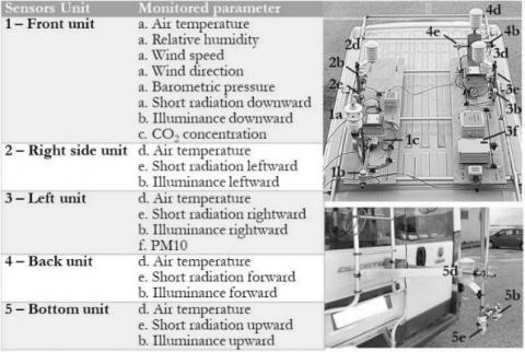
Two different mobile monitoring systems were used simultaneously in this campaign. The first one, the pedestrian transect, is a wearable device specifically designed to monitor outdoor environments on a hyperlocal scale from a pedestrian perspective [17]. This system consists of a set of calibrated sensors joint in a backpack that can be transported to every spot within a city, which is especially useful in historical and protected areas where vehicles sometimes cannot access. This wearable is capable to monitor air temperature, relative humidity, atmospheric pressure, wind velocity and direction, global solar radiation, illuminance, particulate matter concentrations (PM1.0, PM2.5, and PM10), and CO2, O3, and NO2 concentrations. Moreover, it also counts with a GPS to associate a geographic position to each measurement that is made. Data are retrieved every five seconds, guaranteeing spatial and temporal resolution to the monitoring performed with this equipment. The technical specifications of the sensors are summarized in Table 1 and additional details about the wearable monitoring system are described in the studies of ref. [17].
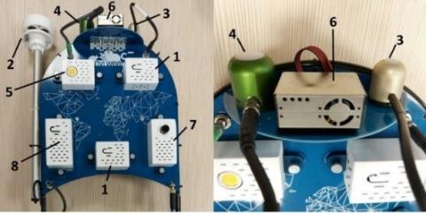
The other monitoring system is a vehicle-based station projected for intra-urban microclimate monitoring. The sensors of this station are positioned in five hosting units. Shortwave radiation and illuminance are measured by different sensors positioned in all the five units and are oriented towards the (1) sky, (2) right, (3) left, and (4) backside of the vehicle, and towards (5) the street pavement. Each unit also has a sensor to measure air temperature. Unit 1 also counts with sensors dedicated to monitoring relative humidity, wind speed and direction, barometric pressure, and CO2 concentration. A sensor to monitor PM10 concentration is positioned in unit 3. Besides this, a GPS antenna is also installed on the vehicle. All measurements are registered every 10 seconds, which ensures temporal and spatial granularity to these data. The technical characteristics of the sensors are reported in Table 2. More technical information related to the vehicle-based monitoring system is presented in the studies of ref. [16, 18].
2.3 Data analysis
The post-processing of the experimentally collected data provided different maps concerning microclimatic parameters’ variation in the investigated areas. These last were identified by morphological and typological features also connected to building form/dimensions. Results of the microclimatic maps comparison showed the different granularity of the parameters measured by the two systems.
Table 1. Sensors in the wearable monitoring equipment and their technical specifications [17]
|
ID (Figure) |
Parameter |
Technical specifications |
|
1 |
Air temperature |
Operation range: -40℃-85℃ Absolute accuracy: ± 1℃ at 0-65℃ |
|
1 |
Relative humidity |
Operation range: 10%-90% at 0-65℃ Absolute accuracy: ± 3% at 20-80% RH Response time: 1 s |
|
1 |
Atmospheric pressure |
Operation range: 300 hPa – 1,100 hPa at 0-65℃ Sensitivity error: ± 0.25% |
|
2 |
Wind velocity |
Operation range: 0.25 Kt – 80 Kt Sensitivity: 0.25 Kt Resolution: 0.1 Kt Output update: 2 per second |
|
2 |
Wind direction |
Sensitivity: ± 1° Resolution: 1° Output update: 2 per second |
|
3 |
Global solar radiation |
Measurement range: 0-2,000 W/m² Calibration uncertainty: ± 5% Detector response time: 0.5 s Spectral range: 385 nm – 2,105 nm |
|
4 |
Illuminance |
Measurement range: 0 – 150,000 lx Calibration uncertainty: ± 5% Response time: 0.6 s |
|
5 |
CO2 concentration |
Accuracy: ± 2% at 20°C, 1 bar pressure, applied gas 2.5% volume CO2 Response Time t90: < 30 s at 20℃ |
|
6 |
Particulate matter concentration (PM1.0, PM2.5 and PM10) |
Effective range (PM2.5 standard): 0 – 500 μg/m³ Resolution: 1 μg/m3 Maximum consistency error (PM2.5 standard): ± 10 μg/m³ at 0–100 μg/m³; ± 10% at 100–500 μg/m³ Total response time: < 10 s |
|
7 |
O3 concentration |
Sensitivity (nA/ppm at 1ppm O3): -200 to -650 Response time (t90 (s) from zero to 1 ppm O3): < 80 s |
|
7 |
NO2 concentration |
Sensitivity (nA/ppm at 2ppm NO2): -175 to -500 Response time (t90 (s) from zero to 2 ppm NO2): < 80 s Range (ppm NO2 limit of performance warranty): 20 ppm |
|
8 |
GPS unit |
Horizontal spatial accuracy: 2.5 m |
Table 2. Sensors in the vehicle-based monitoring equipment and their technical specifications [18]
|
Unit (Figure) |
Parameter |
Technical specifications |
Orientation |
|
1 |
Air temperature |
Accuracy: ±0.3° @ 20° resolution: 0.1° |
- |
|
Relative humidity |
Accuracy: ±2% @ 20° (10–60% RH) resolution: 1% |
- |
|
|
Wind velocity |
Accuracy: ±3% @ 40 m/s resolution: 0.001 m/s |
- |
|
|
Wind direction |
Accuracy: ±3° @ 40 m/s resolution: 1° |
- |
|
|
Barometric pressure |
Accuracy: ±0.5 hPa @ 25° resolution: 0.1 hPa |
- |
|
|
Solar radiation |
Spectral range: 300–3,000 nm 1 W/m2 |
Downward |
|
|
1, 2, 3, 4, 5 |
Illuminance |
Range: 0–10,000 lx |
Downward, leftward, rightward, forward, upward |
|
1 |
CO2 concentration |
Range: 0–2,000 ppm accuracy: ± (50 ppm +2% of measured value) |
- |
|
2, 3, 4 |
Air temperature |
Resolution: 0.1° |
- |
|
2, 3, 4, 5 |
Solar radiation |
Spectral range: 285–3,000 nm calibration uncertainty: < 1.8% |
Leftward, rightward, forward upward |
|
3 |
Particulate matter concentration (PM10) |
Resolution: 1/4,096 Accuracy: < 1% |
- |
Since the paths lasted more than one hour to be completed, an effect of elapsed time on the outdoor air temperature was expected. Therefore, a time-dependency correction was applied before analyzing the variation of the air temperature along the paths. The paths started and finished at the same spot. Thus, the correction consisted in subtracting the air temperature at the beginning of the path by the temperature at the end, and dividing this difference by the time spent to complete the route. Through this, a rate of temperature change in time in [℃/s] was obtained for each path at the three different times of the day they were completed. Then, every measurement made by each monitoring system was corrected according to the respective rate.
The external air temperature and global solar radiation data, collected at the intra-urban scale by using the vehicle-mounted station, allowed the calculation of the sol-air temperature (Tsol-air) variations. The basic formula of Tsol-air as suggested by [19, 20] was applied to the case study taking into account the monitored built environment with a typical canyon shape. Consequently, the sky view factor of any vertical surface/element was lower than 0.5 for most of the measurement time, and assuming precautionary conditions, the F_r value of zero was taken for a preliminary analysis. Therefore, the simplified expression of Tsol-air is provided by Eq. (1) [19, 20]:
$T_{\text {sol-air }}=T_{\text {air,e }}+\left(\alpha \cdot I_{\text {sol }} / h_c\right)\left[{ }^{\circ} \mathrm{C}\right]$ (1)
with Tair,e outdoor air temperature [°C] measured at each point of the path by the thermo-hygrometer in the front unit station mounted on the vehicle, Isol global solar radiation [W/m2] measured by the pyranometer in the front unit station mounted on the vehicle, hc heat transfer coefficient or external liminal adductance [16].
The parameter α (i.e. the hemispheric mean absorption coefficient of different materials detected during the paths with the vehicle [-]) was calculated in each point of the path using the incident global solar radiation measured by the aforementioned pyranometer and differently oriented pyranometers mounted on the two sides of the same vehicle, for the reflected solar radiation measurements due to all the vertical surfaces/walls at the canyon boundaries.
For this calculation, as a precautionary condition, the global solar radiation incident on the vertical surfaces was assumed to be equal the one collected on the horizontal surface of the vehicle roof.
The knowledge of the distribution of the variation (maps and graphs) of the temperature value indicates the local overheating effect of the air but also of the heat input that contributes to the increase of the UHI because it represents the thermal gain of the different opaque surfaces characterized by equally different mean hemispheric absorption coefficients. Therefore, it allows identifying the areas of potential control of the urban albedo with a view to a conscious regeneration and resilience for green sustainable design.
The sol-air temperature values calculated were used for the assessment of the induced external thermal load (∆T) variations, based on the following Eq. (2):
$\Delta T=T_{\text {air }, i, \text { design }}-T_{\text {sol-air }}\left[{ }^{\circ} \mathrm{C}\right]$ (2)
with $\mathrm{T}_{\text {air,i,design }}$ design fixed indoor air temperature for summer, as suggested [21], and Tsol-air, the sol-air temperature in each point of the path [℃] calculated as above mentioned. This analysis provided the quantification of the thermal load due to building air-conditioning released in the urban areas along the investigated path.
The temperature gradient calculation due to the difference between the design internal air temperature and the external one provided the knowledge of the real effects of climatic fluctuations, connected to the UHI, on the acceptability of the internal environment conditions by the users and then the potential cooling demand of buildings.
It also provided indications on how to develop and implement an adaptive management and regulation system of the plants to reduce the thermal gradient by increasing the value of the internal design temperature according to the trend of the external one. For instance, an internal temperature of 28℃ would still allow to guarantee acceptable conditions for users, lower health risks due to lower thermal shocks, but also a significant energy saving linked to a lower environmental impact and, therefore, true energy sustainability. This outcome would be also useful for the evaluation of anthropogenic heat in fostering the UHI phenomenon in different urban environments.
The city center of Florence in Italy was selected as the case study for this experiment. Florence is a relatively large city with high historical value and a vast number of cultural heritage sites. It has around 368,000 inhabitants (Istat 2021 data [22]) and more than ten million tourists visit the city every year, especially in summer. Therefore, this research was focused on the summer period, when the UHI effects are more perceived combined with more crowded areas.
The two mobile monitoring systems followed two different paths within the city center. The vehicle monitored the microclimate around the area of the historic city center to finally cross it (Figure 1a). The wearable station monitored the microclimate inside the historic city center using the paths of the typical touristic flows (Figure 1b, 1c). Crucial findings of a sunny day at the end of summer, i.e. September, 15th 2021, are provided for the three time slots previously mentioned. The average microclimate conditions observed in this day in the city of Florence are summarized in Table 3. These data are provided by a fixed weather station located inside the city center of Florence at Fondazione Osservatorio Ximeniano [23].
Table 3. Average microclimate conditions observed in the city center of Florence on September 15th, 2021
|
Parameter |
Average value |
|
Air temperature [℃] |
23.1 |
|
Relative humidity [%] |
48.4 |
|
Wind velocity [m/s] |
1.8 |
|
Wind direction [°] |
188.5 |
|
Solar radiation [W/m2] |
271.6 |
|
Precipitation [mm] |
0.0 |
During the monitoring campaign a green installation – a greenery spot – was settled by the municipality in the square of the cathedral S. Maria del Fiore, near the Baptistery (Figure 1c). Particular attention was paid to the pedestrian monitoring of microclimatic data in this area to evaluate the potential passive cooling, due to the effect of adiabatic air saturation, provided by the greenery on the local microclimate.
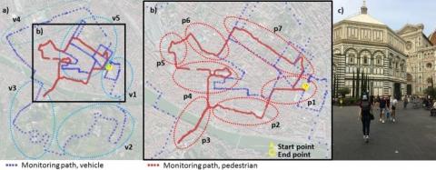
Figure 1. a) Vehicle monitoring path, b) pedestrian monitoring path, and c) monitoring campaign in the city center of Florence
Vehicle and pedestrian paths (Figure 1a, 1b) started and finished at the same spot, a university area (zones v1 and p1 on the map). This a mostly built up area, with large streets and a few small green spots spread around. The vehicle system, then, completed the path passing by an uphill road (v2), up to 130 m a.s.l., in a mainly green area, with plants at the edge of the road that provide some shading and with sparse constructions; a downhill road (v3), down to 50 m a.s.l., as the city center. The latter zone has initially characteristics similar to v2, while in the last part the vehicle passed inside two narrow urban canyons. Thereafter, the path continued in proximity of the main train station of the city in an open area with large streets (v4). Finally, the vehicle crossed the inner city center, a densely built area mainly characterized by narrow streets – except for the main square of the city (v5).
The pedestrian path, after the university area, followed through medieval narrow streets and the open square of Santa Croce in a fully built area (p2); the Ponte Vecchio bridge, i.e. a highly touristic and fully built area (p3); the main square of the city (Santa Maria del Fiore cathedral), through larger streets and open areas (p4). As above-mentioned, a temporary green spot was installed in this area at that time. Therefore, the pedestrian path continues towards the fully built area of the main train station of the city through a large street (p5); the main craft market of the city (S. Lorenzo), i.e. a fully built area with narrow streets (p6); and, finally, historical areas with large streets and gardens (p7).
4.1 Variation of microclimate parameters
This section presents the observed variation in the air temperature (corrected considering the elapsed time of each route) along the paths of both the experimental campaigns.
Regarding the pedestrian path, at 8:00 am, the temperature varied by 1℃ along the route, with the highest temperatures registered in the markets area (p6) and the lowest in the main square area (p4) that is shaded. At 12:00 pm, the highest temperatures were verified in zones p2 and p3 (Figure 1b), and at 4:30 pm in zones p2, p3, and p4. All these areas were the most crowded ones during these periods, then the higher temperatures could be associated with the more intense anthropogenic activities in these places. At 12:00 pm and 4:30 pm, the lowest temperatures were verified nearby an urban park in zone p7. Overall, air temperature varied by 3.3℃ during the 12:00 pm walk and 2.4℃ at 4:30 pm.
The green installation with an area of around 100 m² positioned in the main square (p4) did not have any effect on air temperature. On the other hand, it was observed a cooling effect around the urban park in zone p7, which has an area of approximately 25,000 m². Indeed, it was already stated that greenery has an important role in mitigating urban microclimate, but when it covers a small area, its mitigation capability is lower in comparison to large urban parks [24].
Concerning the vehicle-based monitoring, the temperature range was about 4℃ at 8:00 am. The highest values were measured in the inner region (zone v5), which is more densely built, and in the southern area (v2), which is an open field facing East. On the contrary, at 12:00 pm, the hotter area is zone v2 and the coldest is zone v5. This difference can be associated with solar radiation contribution: the open field makes zone v2 to be more exposed resulting in a temperature increase. Zone v5, characterized by high building density, receives a lower amount of solar radiation, and for this reason, was colder. The range in temperature at this time of the day was around 3.5℃. At 4:30 pm, the temperature was more homogeneous along the path (approximately 2℃ of difference between the hottest and coolest spots), with higher temperatures registered close to the train station (zone v4), which corresponds to the area with more intense anthropogenic activities.
Larger temperature variations were observed along the vehicle-based path in comparison to the pedestrian one. This contrast can be justified by the longer path completed by the vehicle system, which allowed to monitor larger and more diverse areas with this equipment. Another reason seems to be the altitude variation experienced by the system, a factor that influences the air temperature. The path crossed with the pedestrian device, was indeed, flatter. However, even though the variation in the air temperature observed with the pedestrian equipment was smaller, it is still significant considering that the measurements were taken within the same urban environment. This emphasizes the importance of performing environmental monitoring on a hyperlocal scale to address these differences.
4.2 The Sol-air temperature
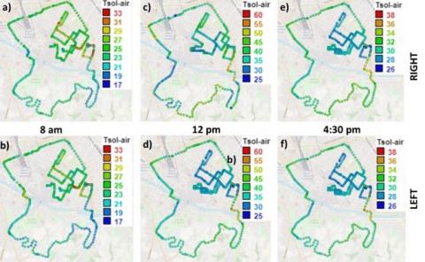
The calculation of sol-air temperature (Tsol-air) was carried out using the vehicle-based monitoring data at 8:00 am, 12:00 pm, and 4:30 pm, to assess the variation in space and during the day (Figure 2). The parameter was calculated for both sides of the monitored urban canyons. A standard value of 23 W/m2 K was considered for the heat transfer coefficient (hc) for external vertical surfaces [19].
Figure 2. Sol-air temperature maps
At 8:00 am, a significant difference between the two sides was observed along the whole path up to about 9.9℃. However, the average difference is equal to about 1.5℃.
Moreover, the Tsol-air rarely corresponds to the outdoor air temperature, with maximum and average differences equal to about 10.5℃ and 3.2℃, respectively.
At 12:00 pm, the highest difference among temperatures was observed, both in space and among sol-air temperatures and outdoor air temperatures. The difference between the two orientations is up to about 20.1℃, with an average value of about 3.1℃. Moreover, the variation with respect to outdoor air temperature is more than 30℃, with an average difference equal to almost 10℃, confirming the role of solar radiation in affecting the heat transfer in summer. At 4:30 pm, a much lower difference was found between the two sides, up to about 4.3℃, and only in the first 30 minutes of monitoring, when the solar radiation was still reaching the vertical surfaces. Thereafter, negligible differences were observed between the two sides with an average difference along the path equal to about 0.4℃. Also, the variation with respect to the outdoor air temperature is the lowest, with minimum values observed after 5:15 pm (average difference equal to about 1.8℃).
4.3 Induced external thermal load
The induced external thermal load ($\Delta \mathrm{T}$) was calculated starting from the values of sol-air temperature at 8:00 am, 12:00 pm, and 4:30 pm for the two sides of the monitored urban canyons. The design indoor air temperature was considered equal to 25℃ in summer [21].
In the morning (at 8:00 am), the sol-air temperature is almost always lower than the design indoor air temperature up to about 5.8℃, stressing the lack of need for cooling and the availability of free-cooling through natural ventilation. This condition was observed up to around 9:30 am when there is the switch of the trend up to 7.8℃, already. At 12:00 pm, the external Tsol-air is always higher that the design indoor air temperature, with peaks up to more than 30℃.
This extreme difference may have been influenced by the assumptions made in the calculations. Anyway, the average difference is equal to about 11.7℃. In the afternoon (4:30 pm), the sol-air temperature is again always higher that the indoor design air temperature. However, the differences – even if non-negligible – are lower and up to about 12.1℃.
Moreover, after around 5:15 pm, when the absence of the effect of solar radiation was observed, the difference is reduced to about 4-3℃.
In this work, we exploit the potential of portable pedestrian and vehicular environmental monitoring systems for providing new insight into the historical city of Florence, where tourism resilience to climate change may report key consequences on the citizenship well-being and the economic prospect of the city – strictly related to the obtained commercial income during the warmest seasons of the year.
Results from the microclimate assessment, allowed to identify local variations in terms of sol-air temperatures and induced external loads within the city pattern, which, in turn, highlighted notable urban areas particularly prone to local overheating phenomena due to a combination of intense anthropogenic activities and elevated solar gains, where UHI mitigation techniques could be exploited.
More in general, the potential applications of the monitored microclimate and the available human centric collected data may be envisaged as follows: i) possibility for hyperlocal mapping of urban microclimate variation in cities according to the variation of geometry, morphology, surfaces thermal performance, density of anthropogenic forcing people, etc., while also comparing different tools characterized by different granularity such as also other monitoring systems (fixed weather stations, satellite measurements, etc.); ii) analysis of citizens’ and tourists’ risk and their health conditions in terms of resilience and morbidities, and correlation of environmental parameters with human behavior and perception, also as a support for the development of information campaigns for tourists and citizens; iii) more granular evaluation of the role of anthropogenic heat on microclimate variation in urban areas and correlation with city GIS database; iv) better precision energy analysis of the built environment, thanks to the sophisticated building physics reconstruction through this hyperlocal reconstruction; v) analysis of solar vulnerability in historic city centers and solar availability for both renewables installation and natural lighting.
This work was supported by the European Union through the founded Project Horizon 2020 innovation programme under the grant agreement No. 792210 (GEOFIT), and the Horizon Europe ERC Grant HELIOS (GA 101041255). The research was further supported by the Italian Ministry by the young researcher PRIN project NEXT.COM (20172FSCH4_002). The authors would like to thank the Italian funding programme Fondo Sociale Europeo REACT EU – Programma Operativo Nazionale Ricerca e Innovazione 2014-2020 (D.M. n.1062 del 10 agosto 2021) for supporting their research through projects “Efficientamento energetico e rinnovabili nella catena del freddo e nel sistema edificio-impianto” and “Red-To-Green”; finally acknowledges are due to the PhD school in Energy and Sustainable Development from the University of Perugia (Italy).
[1] Ravanelli, R., Nascetti, A., Cirigliano, R.V., Di Rico, C., Monti, P., Crespi, M. (2018). Monitoring urban heat island through google earth engine: Potentialities and difficulties in different cities of the United States. International Archives of the Photogrammetry, Remote Sensing and Spatial Information Sciences - ISPRS Archives, XLII-3: 1467-1472. https://doi.org/10.5194/isprs-archives-XLII-3-1467-2018
[2] Kaloustian, N., Diab, Y. (2015). Effects of urbanization on the urban heat island in Beirut. Urban Climate, 14: 154-165. https://doi.org/10.1016/j.uclim.2015.06.004
[3] Okwen, R., Pu, R., Cunningham, J. (2011). Remote sensing of temperature variations around major power plants as point sources of heat. International Journal of Remote Sensing, 32(13): 3791-3805. https://doi.org/10.1080/01431161003774723
[4] Polydoros, A., Cartalis, C. (2015). Assessing the impact of urban expansion to the state of thermal environment of peri-urban areas using indices. Urban Climate, 14: 166-175. https://doi.org/10.1016/j.uclim.2015.10.004
[5] Nuruzzaman, M. (2015). Urban heat island: Causes, effects and mitigation measures - a review. International Journal of Environmental Monitoring and Analysis, 3(2): 67-73. https://doi.org/10.11648/j.ijema.20150302.15
[6] Chen, X., Zhang, Y. (2017). Impacts of urban surface characteristics on spatiotemporal pattern of land surface temperature in Kunming of China. Sustainable Cities and Society, 32: 87-99. https://doi.org/10.1016/j.scs.2017.03.013
[7] Ashtiani, A., Mirzaei, P.A., Haghighat, F. (2014). Indoor thermal condition in urban heat island: Comparison of the artificial neural network and regression methods prediction. Energy and Buildings, 76: 597-604. https://doi.org/10.1016/j.enbuild.2014.03.018
[8] Wang, G.Q., Zheng, B.H., Yu, H.W., Peng, X.G. (2019). Green space layout optimization based on microclimate environment features. International Journal of Sustainable Development and Planning, 14(1): 9-19. https://doi.org/10.2495/SDP-V14-N1-9-19
[9] Meignen, F., Martínez, A., Martí, N. (2020). Greenery in intermediate spaces of the dwellings in the city of Barcelona. International Journal of Sustainable Development and Planning, 15(6): 801-811. https://doi.org/10.18280/ijsdp.150602
[10] Omodero, C.O. (2021). Fiscal decentralization and environmental pollution control. International Journal of Sustainable Development and Planning, 16(7): 1379-1384. https://doi.org/10.18280/ijsdp.160718
[11] Lam, Y.F., Ong, C.W., Wong, M.H., Sin, W.F., Lo, C.W. (2021). Improvement of community monitoring network data for urban heat island investigation in Hong Kong. Urban Climate, 37: 100852. https://doi.org/10.1016/j.uclim.2021.100852
[12] Levinson, R., Ban-Weiss, G., Chen, S., Gibert, H., Goudy, H., Ko, J., Mohegh, A., Rodriguez, A., Slack, J., Taha, H., Tang, T., Zang, J. (2019). Monitoring the urban island effect and the efficacy of future countermeasures heat. In: FINAL PROJECT REPORT Monitoring the Urban Heat Island Effect and the Efficacy of Future Countermeasures. Lawrence Berkeley National Laboratory. Report #: CEC-500-2019-020. http://dx.doi.org/10.20357/B7DW2D
[13] Halder, B., Bandyopadhyay, J., Banik, P. (2021). Monitoring the effect of urban development on urban heat island based on remote sensing and geo-spatial approach in Kolkata and adjacent areas, India. Sustainable Cities and Society, 74: 103186. https://doi.org/10.1016/j.scs.2021.103186
[14] Sismanidis, P., Keramitsoglou, I., Kiranoudis, C.T. (2015). A satellite-based system for continuous monitoring of Surface Urban Heat Islands. Urban Climate, 14: 141-153. https://doi.org/10.1016/J.UCLIM.2015.06.001
[15] Xu, H., Chen, Y., Dan, S., Qiu, W. (2011). Dynamical monitoring and evaluation methods to urban heat island effects based on RS&GIS. Procedia Environmental Sciences, 10: 1228-1237. https://doi.org/10.1016/J.PROENV.2011.09.197
[16] Kousis, I., Pigliautile, I., Pisello, A.L. (2021). A mobile vehicle-based methodology for dynamic microclimate analysis. International Journal of Environmental Research, 15: 893-901. https://doi.org/10.1007/s41742-021-00349-7
[17] Cureau, R.J., Pigliautile, I., Pisello, A.L. (2022). A new wearable system for sensing outdoor environmental conditions for monitoring hyper-microclimate. Sensors, 22(2): 502. https://doi.org/10.3390/s22020502
[18] Kousis, I., Pigliautile, I., Pisello, A.L. (2021). Intra-urban microclimate investigation in urban heat island through a novel mobile monitoring system. Scientific Reports, 11: 9732. https://doi.org/10.1038/s41598-021-88344-y
[19] Holman, J.P. (2010). Heat Transfer. McGraw-Hill, New York.
[20] O’Callaghan, P.W., Probert, S.D. (1977). Sol-air temperature. Applied Energy, 3(4): 307-311. https://doi.org/10.1016/0306-2619(77)90017-4
[21] CEN 2019 EN 16798-1:2019 – Energy performance of buildings - Ventilation for buildings - Part 1: Indoor environmental input parameters for design and assessment of energy performance of buildings addressing indoor air quality, thermal environment, lighting and acoustics - Module M1-6.
[22] Italian National Institute of Statistics (ISTAT) Istat. https://www.istat.it/en/, accessed on Jul. 15, 2022.
[23] Fondazione Osservatorio Ximeniano di Firenze. https://ximeniano.it/, accessed on Jul. 25, 2022.
[24] Rosso, F., Pioppi, B., Pisello, A.L. (2022). Pocket parks for human-centered urban climate change resilience: Microclimate field tests and multi-domain comfort analysis through portable sensing techniques and citizens’ science. Energy and Buildings, 260: 111918. https://doi.org/10.1016/j.enbuild.2022.111918