Ruslan Omirgaliyev | Nurkhat Zhakiyev* | Nazym Aitbayeva | Yerbol Akhmetbekov
© 2022 IIETA. This article is published by IIETA and is licensed under the CC BY 4.0 license (http://creativecommons.org/licenses/by/4.0/).
OPEN ACCESS
The environmental situation in the capital city is always in the focus of attention of the municipal authorities of the city and is one of the most important factors influencing the decisions. The capital of Kazakhstan, Nur-Sultan, consumes heat energy generated from fossil fuel, and one of the major problems is an extremely cold and long winter. The GHG emissions and particle matters from the coal-based Combined Heat and Power plant have a significant impact on the environment as smog, particularly in the heating season. This work analyses spatial high-resolution Big Data collected from the metering points of 385 houses and 62 heat transmission contours across a city during the heating season. The temporary resolution was 10 minutes i.e., 8754 rows for 5 months (Jan-May). There are shown the findings of the correlation rates analysis between heat energy consumption by zones of Nur-Sultan and ambient temperature, as well as non-efficient zones with substantial losses. In this paper for developing the prediction tools for the Smart City heat consumption there were used mixed modelling methods and machine learning approaches, such as Linear Regression, K-neighbours Regressor, and Random Forest Regressor models. These obtained results could be helpful for predicting optimal pumping pressure for each distribution network using machine learning technologies and finding overheated contours in real time.
machine learning method, heat energy, heat network, Random Forest Regressor, Kazakhstan
According to reports [1, 2] by 2050, urbanization is expected to increase to 70%, respectively. The rapid development in the transition to renewable energy sources and higher energy efficiency encourages researchers to look for new solutions from different fields of science, including IT. The effective use of information and communication technologies (ICT) is urgently needed to adequately manage data analysis, data transmission, and the effective implementation of complex strategies to ensure the smooth and safe operation of the city [3].
Digitalization can become a key element in solving several issues related to ecology, management, and legislation. Global warming is a major ecological concern for humanity, and one of its causes is the rapid increase in energy consumption. To address this issue, it is crucial to change the attitude and behaviour toward the environment and the use of natural resources, including energy [4]. Various innovative measures in the field of climate protection are currently being implemented. An innovative way of analysing heat consumption data is used for the decision-making process at the level of urban planning. Types of heat supply and their application are displayed after an in-depth analysis of the thermal energy [5]. An analysis of key literature sources on this issue helps to conclude that the main obstacles to the successful implementation of IT technologies are problems associated with efficient access to data, their collection, and exchange. For example, Danish researchers identify several barriers: strategic, economic, legal, conceptual, technical: usability, discoverability and accessibility [6]. Concerning the technical side of the issue, the researchers state that a large amount of data is difficult to process, and slowdown causes losses by having to wait for data from some producers before making heating plans [7].
The urgency of the topic is based on the initiative “Development of Energy-Saving Policy” under the Strategic Development Program of Nur-Sultan 2050 approved in 2019 [8]. According to this policy, it is planned to implement the regulation in the field of energy-saving; a continuous audit of engineering networks will be carried out using a complex of predictive analytics based on digital technologies to reduce losses and prevent unauthorized consumption. As a result of this policy, utility costs are expected to be reduced by energy-efficient buildings, utility bills for households will be reduced, and the health status of low-income residents will improve. The average indoor temperature will increase during the cold season. Reducing the basic heating requirement in verified rooms to one-quarter of the current level can be realized by modernizing buildings using passive design concepts. In all cases, it is necessary to use insulation of exterior walls and combine it with the concepts of natural ventilation and shading of openings [9].
The relevance of this work stems from the necessity to develop and implement technical methods for modelling and analysing energy resource consumption processes in order to effectively manage energy supply to buildings and structures. This requires the analysis of a large amount of data in real-time with the use of modern information technologies, intelligent decision support systems, and energy management of buildings. The computer-aided power supply control system allows for a complete and objective analysis of the consumption of heat and electricity by buildings and structures, considering weather and climate conditions. Monitoring the heat consumption of a particular object includes the process of constant comparison of data on heat consumption with meteorological and other data, such as the number of people, the state of pipeline insulation, etc. This procedure analyses the efficiency of heat supply systems to determine potential savings in heat energy costs [10, 11]. This article considers machine learning methods to predict the consumption of thermal energy by city zones and its correlation with the uncertainties of ambient temperature and wind. Three types of regression models (Linear Regression, K-Neighbours Regressor, Random Forest Regressor) were used to determine the correlation and compare the training and testing results.
In 2011, the Smart Energy System was developed. This concept plays an important role for 100% renewable energy systems for the synergy of energy storage and low-cost heat sources. This project explored options for scenarios with a particular focus on renewable energy in transportation in the context of limited access to bioenergy [12].
The use of formalized system description for the analysis of energy and environmental policy issues is carried out with the help of modeling of energy systems. In the modeling of electric power systems, it is necessary to understand the importance of complete data collection and analysis for entering into the model [13].
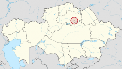
Nur-Sultan city is located in the center of the Eurasian continent. The climate is extreme continental and winter duration is 6 months with severe conditions. The average temperature in January is 16-18℃ below zero, in July -plus 19-21℃ which means that this city is the second coldest capital in the world after Mongolia Republic (Ulaanbaatar).
The wind regime of Nur-Sultan is stable. According to the analysis of wind vector data of Astana International Airport weather station, the average annual wind speed is 5 m/s for both heating and non-heating seasons. The prevailing winds are mostly to the northwest. The analysis of the frequency of wind direction shows that from South-West direction for a non-heating season and from East-North direction for a heating season were the most frequent directions correspondingly.
For providing heat based on coal energy there are two CHPP sources of heat energy. The centralized heating system in Nur-Sultan, which provides heat through the centralized heating network by zone and has a total installed heat capacity of 2840 Gcal/h and an available capacity of 2580 Gcal/h, includes almost all multi-storey residential and public buildings and primarily uses coal as a fuel.
The total length of heating networks is 882,6 km (Table 1), including ~240 km of main heating network, ~490 km of district heating network, ~152 km of the steam pipeline network (Table 1).
Heat consumption for municipal needs of enterprises has almost doubled (by 44%) and in 2020 amounted to 9.3 million GСal of heat energy. Such an increase in volumes is associated with several factors: the early start of the heating season, climatic conditions of the city, an increase in heating loads due to newly connected consumers, steam consumption increase by industrial enterprises. Since 2011, the average daily supply of heat energy per 1000 inhabitants has grown from 8.2 to 9.4 GСal.
Over the past eight years, the volume of heat consumption through centralized heat and steam pipelines has grown by 40.4% and amounted to 8.48 million Gcal in 2021 (Figure 1). The increase in the level of heat consumption is due to the high rates of population growth and intensive housing constructions. With an increase in the length of the heating networks, heat losses increase, which is due to the outdated infrastructure. The actual amount of heat losses is about 12%.
Data Sources: Bureau of National Statistics of the Republic of Kazakhstan www.stat.gov.kz and the municipally government: www.a-tranzit.kz.
*Data for 2021 not devided by categories yet.
Figure 1. The current state of heat energy consumption by categories, thousand GCal
The consumption of heat energy for heating $Q_{h.nor}$ for a certain period of time and the calculated maximum heat load for heating $Q_{h.max}$, are determined by the following Equations:
$\mathrm{Q}_{\mathrm{hrs}}^{\mathrm{h}}=\alpha * \mathrm{~V}_{\mathrm{out}} * \mathrm{q}_{\mathrm{h}} *\left(\mathrm{t}_{\mathrm{in}}-\mathrm{t}_{\mathrm{out}}\right) *\left(1+\mathrm{K}_{\mathrm{inf}}\right) * 10^{-6}[\mathrm{MWt}]$ (1)
$\mathrm{Q}_{\mathrm{h} . \max }=\mathrm{Q}_{\mathrm{hrs}}^{\mathrm{h}}=* 0.8598 \quad[\mathrm{GCal} / \mathrm{h}]$ (2)
$Q_{h . n o r}=Q_{h . \max } * \frac{\left(t_{\text {in }}-t_{a v}\right)}{\left(t_{\text {in }}-t_{\text {out }}\right)} * 24 * Z_{0} \quad[\mathrm{GCal} / h]$ (3)
where, Z0 – duration of the period under consideration, day; tin – average internal air temperature of heated premises, ℃ (Celsius degree); tout–calculated outdoor temperature, ℃; Vout– external construction of a building, m3; qh- specific heating characteristic of residential and public buildings at -30℃, Wt/(m3*℃); α– correction factor; tav– average outside air temperature for the period under consideration, ℃; Kinf - the calculated coefficient of infiltration due to thermal and wind pressure.
The estimated infiltration coefficient Kinf is determined by the Eq. (4):
$K_{\mathrm{inf}}=10^{-2} \sqrt{\left[2 g L\left(1-\frac{273+t_{\text {out }}}{273+t_{i n}}\right)+w_{0}^{2}\right]}$ (4)
where, g = 9.81 m/s2- acceleration of gravity; L - height of the building, m; w0- calculated wind speed [m/s].
Table 1. Total length of heating networks in Nur-Sultan city
|
|
Heating season (years) |
|||||||
|
2010 |
2014 |
2015 |
2016 |
2017 |
2018 |
2019 |
2020 |
|
|
The length of heating networks, km |
520 |
550 |
571 |
583 |
687 |
737 |
816 |
882,6 |
Eq. (3) can be represented as:
$\mathrm{Q}_{\text {h.nor }}=\alpha * \mathrm{~V}_{\text {out }} * \mathrm{q}_{\mathrm{h}} *\left(\left(\mathrm{t}_{\text {in }}-\mathrm{t}_{\mathrm{av}}\right) *\left(1+\mathrm{K}_{\text {inf }}\right) * \mathrm{Z}_{0} * 24 * 0.8598 * 10^{-6}\right.$ (5)
Eq. (5) makes it possible to estimate the dependence of heat losses on the average outside air temperature for the period under consideration and the average wind speed w0. The specific heating characteristic of a building with existing methods is determined by reference data, based on the volume and purpose of the building [14, 15] without considering the individual characteristics of the building.
Based on Eq. (5), it is possible to estimate the consumption of thermal energy for a certain period of time with a minor error, but it is preferable to measure it using metering devices built into the automatic control system.
The actual thermal power of the hot water heating system depends on the flow rate and temperatures of the direct and return supply water:
$Q_{h}=G c\left(t_{dir }-t_{i n d}\right)$ (6)
where, G is the water flow in the heating system; c-heat capacity of water; tdir-temperature of the direct supply water entering the heating system; tind-temperature of the return water from the heating system.
With a constant water flow, the actual heat output of the hot water heating system is directly proportional to the temperature difference between the supply and return water. By increasing or decreasing the temperature of the coolant at the heat supply source at a constant flow rate, high-quality heating control is carried out. The data of the devices of modern metering units allows to determine the flow and temperature values of the direct and return network water in real time, as well as the actual thermal power of the building heat supply system:
$Q_{a . c t}=c\left(G_{dir} t_{dir}-G_{i n d} t_{i n d}\right)$ (7)
where, Gdir- consumption of the direct network water entering the metering unit; Gind is the flow rate of return water from the metering unit.
To create comfortable conditions as well as minimal heat consumption and money costs for paying for energy carriers, it is necessary that the heat released in the room fully compensates for the heat losses. Since heat comes to residential buildings and budgetary institutions from the heating system, the equality of the daily heat consumption ($Q_{h.nor}$) and the actual power of the heating system ($Q_{a c t}$) should be met: $Q_{h.nor}=Q_{act.}$. If $Q_{h.nor}<Q_{a c t}$, then there is an overheating - excessive consumption of heat energy, in this case the temperature in the rooms is higher than the set one and is regulated by opening windows and vents. In cases for $Q_{h.nor}>Q_{a c t}$, is an undersupply, to maintain a comfortable temperature in the premises, electric heating devices are used, which is accompanied by excessive consumption of electricity.
Distributions of wind direction frequency for 2020-2021 is shown in Figures 2a and 2b. Wind data used for correlation analyses in the section 4. During the heating season, the wind direction is more often directed from the southwest to the northeast. For this reason, the CHP is located in the northeast of the city. Due to the ubiquity of coal-fired heating in CHPs and in the private sector, there are days with stagnant smog without wind or moderate wind towards the southwest.
(a) Analysis of wind direction frequency, % for 2020 in Nur-Sultan
(b) Analysis of wind direction frequency, % for 2021 in Nur-Sultan
Figure 2. Distributions of wind direction frequency for 2020-2021 (Source: Wolfram Mathematica 12.3)
3.1 Linear regression
Linear regression is a model of the dependence of variable x on one or more other variables (factors, regressors, independent variables) with a linear dependence function [16, 17].
For a given set of m pairs of $\left(x_{i}, y_{i}\right), i=1, \ldots, m$, values of the free and dependent variable, it is required to define a dependence. Linear model assigned as:
$y_{i}=f\left(w, x_{i}\right)+\varepsilon_{i}$ (8)
with an additive random variable $\varepsilon$. Variables x,y take values on the number line $\mathbb{R}$. It is assumed that the random variable is normally distributed with fixed variance $\sigma_{\varepsilon}^{2}$, which does not depend on the variables x,y. Under these assumptions, the parameters w of the regression model are calculated using the least squares method.
The dependency model defines as follows:
$y_{i}=w_{1}+w_{2} x_{i}+\varepsilon_{i}$ (9)
According to the least square’s method, the required vector of parameters $w=\left(w_{1}, w_{2}\right)^{T}$ is a solution to the normal equation:
$w=\left(A^{\mathrm{T}} A\right)^{-1} A^{\mathrm{T}} y$ (10)
where, y-vector consisting of the values of dependent variable $y=\left(y_{1}, \ldots, y_{m}\right)$. The columns of matrix A are substitutions of the values of free variable $x_{i}^{0} \rightarrow a_{i 1}$ and $x_{i}^{1} \rightarrow a_{i 2}, i=1, \ldots, m$. The matrix has the form:
$A=\left(\begin{array}{cc}1 & x_{1} \\ .. & .. \\ 1 & x_{m}\end{array}\right)$ (11)
The dependent variable is restored from the obtained weights and the specified values of the free variable:
$y_{i}^{*}=w_{1}+w_{2} x_{i}$, (12)
Or
$y^{*}=A w$ (13)
To assess the quality of the model, the criterion of the sum of squares of regression residuals, SSE - Sum of Squared Errors is used in Eq. (14):
$S S E=\sum_{i=1}^{m}\left(y_{i}-y_{i}^{*}\right)^{2}=\left(y-y^{*}\right)^{T}\left(y-y^{*}\right)$ (14)
3.2 The K-Neighbors Regressor
The compactness hypothesis reinforces the K Neighbors Regressor model, which is the method's foundation: if the metric of distance between examples is successfully introduced, similar examples are much more likely to belong to the same class than others [18, 19].
In the case of using the classification method, the object is assigned to the most common class among the k-neighbors of the given element, the classes of which are already known. If the method is used for regression, the object is assigned to the average of the k nearest to its objects whose values are already known. The KNN algorithm can be divided into two simple phases: training and classification. The algorithm recollects the observation feature vectors and their class labels during training (i.e., examples). In addition, the algorithm parameter k, which sets the number of "neighbours" to be used in classification, is set. At the classification phase, a new object, for which the class label is not given, is presented. It is determined that k is the nearest in the sense of some metric pre-classified observations. The class to which the majority of the k nearest-neighbor examples belong is then chosen, and the object being classified belongs to the same class.
Table 2. Advantages and Disadvantages of chosen 3 models
|
Model type |
Advantages |
Disadvantages |
Reference |
|
Linear Regression |
1. Interpretability of the model. The linear model is transparent and understandable for the analyst. Based on the obtained regression coefficients, it is possible to assess how this or that factor influences the outcome, and draw additional useful conclusions. |
1. Models only direct linear dependencies, while it is often necessary to create a model of other types of relationships between data. |
[22] |
|
2. Speed and ease of obtaining a model. |
2. The algorithm assumes that the input functions are mutually independent (without collinearity). |
[22] |
|
|
3. Wide applicability. A large number of real processes in the economy and business can be described with sufficient accuracy by linear models. |
3. The algorithm assumes that the input residuals (error) are distributed normally, but cannot always be fulfilled. |
[23] |
|
|
4. Typical problems and their solutions are known for linear regression, tests for evaluating the static significance of the resulting models have been developed and implemented. |
4. Applicable only if the solution is linear. In many real-world scenarios, this may not be the case. |
[24] |
|
|
K-Neighbors Regressor |
1. Resistance to emissions and abnormal values |
1. Does not create any models that summarize previous experience |
[25] |
|
2. The results of the algorithm are easy to interpret. The logic of the algorithm can be understood by experts in various fields. |
2. High labor intensity due to the need to calculate the distances to all examples |
[26] |
|
|
3. The software implementation of the algorithm is relatively simple |
3. Quite computationally expensive because of the use of all available data for classification |
[27] |
|
|
Random Forest Regressor |
1. The ability to efficiently process data with many features and classes. |
1. Large size of the resulting models. |
[28] |
|
2. Insensitivity to scaling (and generally to any monotonic transformations) of feature values. |
2. More computing resources are required. |
[29] |
|
|
3. Internal assessment of the generalizability of the model (test on unselected samples). |
3. Time consuming compared to other algorithms. |
[30] |
|
|
4. High parallelizability and scalability. |
4. The algorithm is prone to overfitting on some tasks, especially on noisy |
[31] |
The problem characteristic of most classification methods is the different importance of features in terms of determining the class of objects. Considering the importance of features in the algorithm may allow for increased classification accuracy. The following formula is used to determine the importance of the feature:
$D_{E}=\sqrt{s_{1} *\left(x_{1}-a_{1}\right)^{2}+s_{2} *\left(x_{2}-a_{2}\right)^{2}+\ldots+s_{p} *\left(x_{p}-a_{p}\right)^{2}}$ (15)
where, si (i = 1...p) is significance factor for the ith attribute and p is the number of features of the original data set.
The KNN algorithm is useful for almost all classification tasks, particularly while estimating the parameters of the probability distribution of data is difficult or impossible.
3.3 Random Forest Regressor
Random Forest Regressor is a machine learning algorithm that uses numerous decision trees on solutions conceived by Leo Breiman and Adele Cutler. Since its invention, it has never undergone changes and is in its original form. Stands out among other classification algorithms by its multipurposeness. The multipurposeness stems from the capacity to solve classification, regression, clustering, anomaly search, and feature selection problems [20, 21].
Each tree should be built in accordance with the following strategy: First, it must take a subsample with the size of the sample from the training sample and, according to this, build trees with individual subsamples; second, a maximum feature from random features is browsed in order to model each splitting; and finally, the most accurate splitting and feature can be selected based on the arranged in advance criterion. The classification of objects is carried out by voting: each tree in the committee assigns the object to one of the classes, and the class with the most votes is the more dominant option.
The optimal number of trees is selected in such a way as to minimize the classifier error on the test sample. If it is not present, the error estimation on samples that are not part of the set is minimized.
Two things are required to get more precise predictions. Firstly, it is crucial to have features with explanatory value. Secondly, predictions of trees and forest itself should not be correlated with each other.
Table 2 represents advantages and disadvantages of 3 different machine learning models.
The dataset contains 8754 lines. Values of min are always 0 when a node is not operational. Values of 0 on the sensors appear in cases of failure of the equipment itself or in cases when the weather conditions are unfavourable (either very cold or very hot). The average is different for each, as these are different contours. There are no null values in this dataset, but there are strings where the value is 0. Therefore, replacing them with null values is the correct method. Figure 3 shows information about this dataset more precisely.
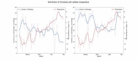
Figure 4 illustrates the changes of an enthalpy with outdoor temperature over 5 months. In this case, Contour-1 – the closest contour to TPP (thermal power plant), while Contour-2 – the farthest.
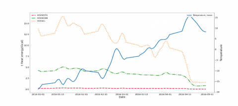
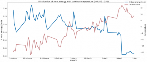
Applying the same logic to the consumers (hereafter Homes), results in the graph shown in Figure 5 (а). House-1 is the farthest consumer from Contour-1, House -251 is the closest one, and House-384 has medium distance from Contour-1. Figure 5 (a) visually indicates that Heat consumption by House-251 is zero, but in Figure 5 (b) it is shown as zoomed correlation.
Enthalpy- 1 decreases with increasing temperature. There is a fluctuation in outdoor temperature in the months of February and March. In general, increasing Enthalpy values affects decreasing outdoor temperatures and vice versa.
$q=\frac{M_{c w} c_{w}\left(t_{o u t}-t_{i n}\right)}{M_{h w}}$ (16)
where, q is the specific amount of heat, kJ / kg; Mcw- the mass of indirect water, kg; cw- specific heat capacity of water, equal to 4.19 kJ / (kg⋅K); tout- water temperature at the output of a contour, ℃;tin- water temperature at the input to the contours, ℃; Mhw- the mass of condensate, kg.
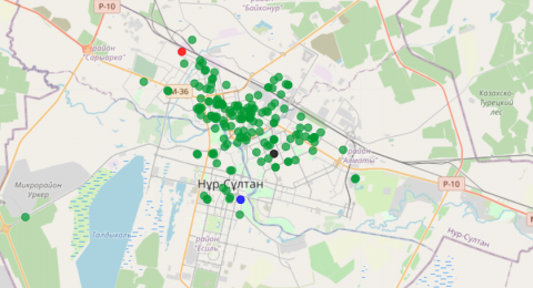
The visualization in Figure 6 shows the dependence of the average hourly temperature and the time of day. The highest rates are observed in the morning from 5 to 10 hours, the lowest in the daytime from 10 to 15 hours. The temperature at the entrance and exit, which is associated with an increase in air temperature. Moreover, Figure 7 depicts the location of houses in Nur-Sultan from the dataset.
The target variable at this point is "Thermal Energy in GCal". Additionally, it is necessary to use the ambient temperature of Nur-Sultan as one of the features.
Figure 8 shows distributions of values for different variables, namely Thermal Energy in Gcal (or Heat Consumption), maximum temperature, minimum temperature on that specific day and speed of the wind. The frequency can be seen on the vertical axis.
From Figure 8 it is seen that 5 m/s wind speed has been repeated 4 times and so on. Figure 9 shows the correlation between these variables. As it is visible from the figure there are more or less good correlations between them.
Figure 3. Descriptive statistics of 4 parameters for each 62 heating contours.
Figure 4. Direct Temperature Changing profile in 24 hours
(a) Distribution of Heat Energy with outdoor temperature for 3 different consumers
(b) Distribution of Heat Energy with outdoor temperature (House-251)
Figure 5. Distribution of Heat Energy
Figure 6. Direct Temperature Changing profile in 24 hours
(a) Nur Sultan on the map of Kazakhstan
(b) The location of 385 metering points in a map of Nur-Sultan city
Figure 7. Map of Nur-Sultan city
Figure 8. Distribution of values: heat consumption in GCal, maximal and minimal outdoor temperatures in Celsius degree
Figure 9. Correlations between input features (heat consumption, temperatures, and wind speed)
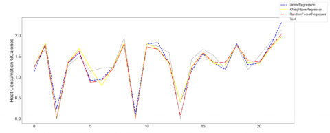
Firstly, it is necessary to use the maximum temperature of the day and the wind speed as input features and predict the target variable using the Linear Regression model, K neighbours Regressor, and Random Forest Regressor, and compare the results. Figure 10 depicts the visualization.
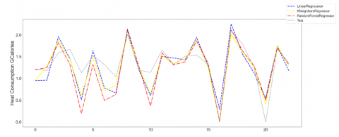
Secondly, the minimum temperature of each day and the speed of the wind were used to predict Thermal Energy (Figure 11).
Thirdly, maximum, minimum temperatures and speed of wind have been taken as input features illustrated in Figure 12.
Then, these 3 models are averaged with a full dataset, which was trained and tested.
Table 3 indicates the comparison of these three models for training and test sets. When predicting the target variable, the dataset was split into training and test sets, namely 80% and 20% respectively. In Table 3, for Linear Regression approach the maximal value of the prediction factor below than 83% of accuracy with or without wind factor. When K-neighbours Regressor or Random Forest Regressor models were used, it is necessary to conclude that the predicted future values increased to 89-90 percent accuracy (green boxes), indicating that ML model algorithms work well for K-neighbours Regressor and Random Forest Regressor models.
Figure 10. Predicting Models with maximum temperature
Table 3. Comparison of prediction accuracies of 3 models (colored focusing results)
|
Model type |
With wind |
Without wind |
Input features |
||
|
Train |
Test |
Train |
Test |
||
|
Linear Regression |
0.81 |
0.54 |
0.79 |
0.58 |
Minimum temperature |
|
0.84 |
0.74 |
0.84 |
0.77 |
Maximum temperature |
|
|
0.83 |
0.82 |
0.82 |
0.83 |
Max and Min temperatures |
|
|
K-neighbours Regressor |
0.89 |
0.53 |
0.83 |
0.90 |
Minimum temperature |
|
0.84 |
0.71 |
0.87 |
0.72 |
Maximum temperature |
|
|
0.87 |
0.77 |
0.87 |
0.81 |
Max and Min temperatures |
|
|
Random Forest Regressor |
0.98 |
0.42 |
0.85 |
0.89 |
Minimum temperature |
|
0.96 |
0.70 |
0.92 |
0.62 |
Maximum temperature |
|
|
0.96 |
0.65 |
0.93 |
0.78 |
Max and Min temperatures |
|
Figure 11. Predicting models with minimum temperature
Figure 12. Predicting models with minimum and maximum temperatures
This paper provides a substantial review of heat energy consumption in general, including the derivation of thermodynamics formulas and the application of machine learning algorithms to forecast future heat energy consumption. The article used machine learning methods to predict the consumption of thermal energy by city zones and its correlation with the uncertainties of ambient temperature and wind. The correlation was determined using training and regression models. These predictions can be useful for analysing heat consumption in Nur-Sultan city and reducing heat losses by minimizing overheating of heat transmission network zones. In addition, spatial high-resolution data collected from the metering points of 385 houses and 62 heat transmission contours across a city during the heating season, were analysed in the work. The results of analysing correlation rates between heat energy consumption by Nur-Sultan zones and an ambient temperature, as well as estimating a minor impact of wind speed, defined the ML model to identify inefficient high-loss zones and overheated zones. In the analysis of the correlation between heat energy consumption by zones and ambient temperature there were used mixed modelling methods and machine learning approaches. These findings might aid in the implementation of Smart City concepts, such as forecasting the optimal pumping pressure for each distribution network using machine learning technologies. In Kazakhstan, this area has not been studied thoroughly and is expected to become a relevant topic in the near future, as global concern about energy is growing and many countries are making efforts to regulate energy- consuming industries, especially buildings and construction. Moreover, these ML-model algorithms can solve any other heat consumption problems for different cities around the world.
This research has been funded by the Science Committee of the Ministry of Education and Science of the Republic of Kazakhstan (Grant No. BR10965311 "Development of the intelligent information and telecommunication systems for municipal infrastructure: transport, environment, energy and data analytics in the concept of Smart City").
[1] O’Dwyer, E., Pan, I., Acha, S., Shah, N. (2019). Smart energy systems for sustainable smart cities: Current developments, trends and future directions. Applied Energy, 237: 581-597. https://doi.org/10.1016/j.apenergy.2019.01.024
[2] Liu, Y., Yang, C., Jiang, L., Xie, S., Zhang, Y. (2019). Intelligent edge computing for IoT-based energy management in smart cities. IEEE Network, 33(2): 111-117. https://doi.org/10.1109/MNET.2019.1800254
[3] Ullah, Z., Al-Turjman, F., Mostarda, L., Gagliardi, R. (2020). Applications of Artificial Intelligence and Machine learning in smart cities. Computer Communications, 154: 313-323. https://doi.org/10.1016/j.comcom.2020.02.069
[4] Bishoge, O.K., Kombe, G.G., Mvile, B.N. (2021). Energy consumption efficiency behaviours and Attitudes among the Community. International Journal of Sustainable Energy Planning and Management, 31: 175-188. https://doi.org/10.5278/ijsepm.6153
[5] Knies, J. (2018). A spatial approach for future-oriented heat planning in urban areas. International Journal of Sustainable Energy Planning and Management, 16: 3-30. http://orcid.org/0000-0003-2944-9285
[6] Jetzek, T. (2016). Managing complexity across multiple dimensions of liquid open data: The case of the Danish Basic Data Program. Government Information Quarterly, 33(1): 89-104. https://doi.org/10.1016/j.giq.2015.11.003
[7] Ben Amer, S., Hjøllund, T., Nielsen, P.S., Madsen, H., Bergsteinsson, H.G., Liu, X. (2021). Energy data: mapping, barriers and value creation. https://orbit.dtu.dk/en/publications/energy-data-mapping-barriers-and-value-creation, accessed on April 1, 2022.
[8] The Strategic Development Program of Nur-Sultan 2050, approved in 2019. https://maslihat01.kz/ru/news/strategiya-razvitiya-2050 (in Russian), accessed on June 1, 2022.
[9] Schelbach, S. (2016). Developing a method to improve the energy efficiency of modern buildings by using traditional passive concepts of resource efficiency and climate adaptation. International Journal of Sustainable Development and Planning, 11(1): 23-38. https://doi.org/10.2495/SDP-V11-N1-23-38
[10] Bogner, K., Pappenberger, F., Zappa, M. (2019). Machine learning techniques for predicting the energy consumption/production and its uncertainties driven by meteorological observations and forecasts. Sustainability, 11(12): 3328. https://doi.org/10.3390/su11123328
[11] Bujalski, M., Madejski, P. (2021). Forecasting of heat production in combined heat and power plants using generalized additive models. Energies, 14(8): 2331. https://doi.org/10.3390/en14082331
[12] Østergaard, P.A., Johannsen, R.M., Lund, H., Mathiesen, B.V. (2021). Latest developments in 4th generation district heating and smart energy systems. International Journal of Sustainable Energy Planning and Management, 31: 1-4. https://doi.org/10.5278/ijsepm.6432
[13] Omirgaliyev, R., Salkenov, A., Bapiyev, I., Zhakiyev, N. (2021). Industrial application of machine learning clustering for a combined heat and power plant: A Pavlodar case study. In 2021 IEEE Int. Conf. on Information and Telecommunication Technologies and Radio Electronics (UkrMiCo), pp. 51-56. https://doi.org/10.1109/UkrMiCo52950.2021.9716605
[14] Chun, B., Guldmann, J.M. (2014). Spatial statistical analysis and simulation of the urban heat island in high-density central cities. Landscape and Urban Planning, 125: 76-88. https://doi.org/10.1016/j.landurbplan.2014.01.016
[15] Fumo, N., Biswas, M.R. (2015). Regression analysis for prediction of residential energy consumption. Renewable and Sustainable Energy Reviews, 47: 332-343. https://doi.org/10.1016/j.rser.2015.03.035
[16] Lei, F., Hu, P.F. (2009). A baseline model for office building energy consumption in hot summer and cold winter region. International Conference on Management and Service Science, pp. 1-4. https://doi.org/10.1109/ICMSS.2009.5301031
[17] Wang, R., Lu, S., Feng, W. (2020). A novel improved model for building energy consumption prediction based on model integration. Applied Energy, 262: 114561. https://doi.org/10.1016/j.apenergy.2020.114561
[18] Parhizkar, T., Rafieipour, E., Parhizkar, A. (2021). Evaluation and improvement of energy consumption prediction models using principal component analysis based feature reduction. Journal of Cleaner Production, 279: 123866. https://doi.org/10.1016/j.jclepro.2020.123866
[19] Ahmad, T., Chen, H. (2019). Nonlinear autoregressive and random forest approaches to forecasting electricity load for utility energy management systems. Sustainable Cities and Society, 45: 460-473. https://doi.org/10.1016/j.scs.2018.12.013
[20] Guo, Z., Zhou, K., Zhang, X., Yang, S. (2018). A deep learning model for short-term power load and probability density forecasting. Energy, 160: 1186-1200. https://doi.org/10.1016/j.energy.2018.07.090
[21] Kafazi, I.E., Bannari, R., Abouabdellah, A., Aboutafail, M.O., Guerrero, J.M. (2017). Energy production: A comparison of forecasting methods using the polynomial curve fitting and linear regression. International Renewable and Sustainable Energy Conference (IRSEC), pp. 1-5. https://doi.org/10.1109/IRSEC.2017.8477278
[22] Ahmed Al-Imam. (2020). A novel method for computationally efficacious linear and polynomial regression analytics of big data in medicine. Modern Applied Science, 14(5): 1-10. https://doi.org/10.5539/mas.v14n5p1
[23] Kwon, S.J., Park, J., Choi, J.H., Lim, J.H., Lee, S.E., Kim, J. (2019). Polynomial regression method-based remaining useful life prediction and comparative analysis of two lithium nickel cobalt manganese oxide batteries. IEEE Energy Conversion Congress and Exposition (ECCE), pp. 2510-2515. https://doi.org/10.1109/ECCE.2019.8912625
[24] Lim, H.I. (2019). A linear regression approach to modeling software characteristics for classifying similar software. IEEE 43rd Annual Computer Software and Applications Conference (COMPSAC), pp. 942-943. https://doi.org/10.1109/COMPSAC.2019.00152
[25] Li, S., Shen, Z., Xiong, G. (2012). A k-nearest neighbor locally weighted regression method for short-term traffic flow forecasting. Intelligent Transportation Systems (ITSC), 15th International IEEE Conference on. IEEE, pp. 1596-1601. https://doi.org/10.1109/ITSC.2012.6338648
[26] Cover, T.M., Hart, P. (1967). Nearest neighbor pattern classification. IEEE Transactions on Information Theory, 13(1): 21-27. https://doi.org/10.1109/TIT.1967.1053964
[27] Zhang, S. (2021). Challenges in KNN classification. IEEE Transactions on Knowledge & Data Engineering, 1:1-1. https://doi.org/10.1109/tkde.2021.3049250
[28] Jaiswal, J.K., Samikannu, R. (2017). Application of random forest algorithm on feature subset selection and classification and regression. 2017 World Congress on Computing and Communication Technologies (WCCCT), pp. 65-68. https://doi.org/10.1109/WCCCT.2016.25
[29] Xiao, Y., Huang, W., Wang, J. (2020). A random forest classification algorithm based on dichotomy rule fusion. 2020 IEEE 10th International Conference on Electronics Information and Emergency Communication (ICEIEC), pp. 182-185. https://doi.org/10.1109/ICEIEC49280.2020.9152236
[30] Dengju, Y., Yang, J., Zhan, X. (2013). A novel method for disease prediction: Hybrid of random forest and multivariate adaptive regression splines. Journal of Computers, 8(1): 170-177. https://doi.org/10.4304/jcp.8.1.170-177
[31] Sutong, W., Yuyan, W., Dujuan, W., Yunqiang, Y., Yanzhang, W., Yaochu, J. (2020). An improved random forest-based rule extraction method for breast cancer diagnosis. Applied Soft Computing, 86: 105941. https://doi.org/10.1016/j.asoc.2019.105941