Atheer M. Al-Saady* | Sedqi E. Rezouki
© 2022 IIETA. This article is published by IIETA and is licensed under the CC BY 4.0 license (http://creativecommons.org/licenses/by/4.0/).
OPEN ACCESS
One of the most critical factors in the implementation of wastewater projects is the development of a plan for the implementation of the project as well as the optimal project delivery method and contract strategy that suits it, which may affect the success of the project. This research aims to explore the joint planning between the project delivery system and contract strategy, with the aim of providing a conceptual framework for designing an appropriate project delivery method and contract strategy. The researcher identified seven basic delivery methods based on a review of previous studies and a questionnaire that were conducted with a group of experts working in sewage projects in Wasit Governorate / Iraq. This research designs PDCS through the analytical hierarchical process This technique has been used for several reasons, including the ease of application and its ability to identify any quality problem, as well as allowing diversity between viewpoints and its ability to bring different opinions together. It can also be applied with many applications such as linear programming and targeted programming, where the main and sub-factors that affect the choice of PDCS are studied. The design process is divided into two stages, the preliminarily design and the detailed design.
project delivery system, contract strategy, multi criteria decision making, AHP
This paper deals with choosing the appropriate method for project delivery. Selection is the key step in defining the overall strategy for project delivery. Project delivery systems refer to the overall processes by which a project is designed, constructed, and/or maintained. Seven project delivery methods have been taken: the design built method (DB), the construction bid design method (DBB), the construction management method (CM), the separate initial contracts (SPC), the turnkey method (T), and the public-private partnership method (PPP) and the method of force account (F.A). To determine which methods are the most appropriate, the owner must take into account several factors related to the decision. Several studies have discussed these methods and presented the advantages and disadvantages of each of them. Gordan [1] suggested using a method to eliminate inappropriate methods. Molenaar et al. [2] develop a web-based selection management system for selecting projects appropriate for a delivery method. Spink [3] discuss the special circumstances that make a delivery system suitable for a given project.
The process hierarchy AHP defines a multi-criteria decision-making method developed by Saaty [4] that is applied to solve unstructured problems in a variety of decision-making situations. The process of hierarchical analysis can be also defined as a method for arranging decision alternatives and choosing the best alternative when the decision maker has multiple goals or criteria on which the decision is based. It is also known as a decision-making tool that analyzes and dismantles the complex problem into a multi-level hierarchical structure of objectives, criteria, sub-criteria and alternatives. Makes an integration of the different quantitative and qualitative measures to combine them in one degree that expresses the arrangement of the alternative among a group of decision alternatives.
AHP is implemented in two phases: hierarchical design and evaluation [4]. In the evaluation stage, the items at the hierarchical level are compared in pairwise comparisons. With respect to each of the elements at the level directly above, a rating scale is used for pairwise comparisons. The comparison process results in a relative order of priorities with respect to the element of the factor with which it was compared. The final order of the elements at the lowest level of the alternatives is obtained by aggregating the contribution of the elements on all the levels in each of the alternatives are carefully discussed in the computational procedure in Satty [4].
This research presents analytical hierarchy process model to determine the appropriate project delivery method. AHP model developed by the paper depends on several factors that can be grouped into the three main categories of project objectives, namely owner requirements, external conditions and administrative aspects.
AHP method was chosen in this research because of the ability of this method to integrate tangible and intangible factors that are difficult to take into account. The second reason is the hierarchical structure. The problem is divided into its component parts through a hierarchy of large elements to small elements.
This research is divided into several sections, where the seven delivery methods are explained, followed by AHP model, the use of the model, and finally the conclusion.
There are many approaches to select PDS and classified into four major groups on the basis of their underlying concepts. Table 1 shows the approaches within each group that will be discussed in this section along with their reference sources. Presentation of the specific methods will focus on their fundamental concepts, merits and limitations [5].
Table 1. Available PDS approach Ibbs and Chih [5]
|
Category |
Approach |
|
Guidance |
Individual PDSs |
|
Alternative comparison of PDS |
|
|
Guidelines and Formalized framework |
|
|
Decision charts |
|
|
Multi-attribute Analysis |
Weighted sum approach |
|
Multi-attribute utility/value theory (MAUT/MAVT) |
|
|
Analytical hierarchical process (AHP) |
|
|
Fuzzy logic approaches |
|
|
Knowledge-/experience based Methods |
case-based reasoning approach (CBR) |
|
Decision support system |
|
|
Mix-method approaches |
AHP/value engineering (VE)/Multi criteria multi screening |
|
AHP/mean utility values |
|
|
MAUT/project database |
|
|
A qualitative assessment/a weighted score approach |
The researcher depends on Multi-attribute Analysis using analytical hierarchical process (AHP) to select an optimal PDS in wastewater projects.
This research attempts to explore the joint planning between PDS and contract strategy (CS), aiming to put forward a conceptual framework for the design of PDCS. In terms of the PDS, the researcher maintain that (DBB, DB, CM-R, SPC, Turnkey, PPP and force account) are the seven fundamental PDS based on the review of previous studies and personal interviews.
This research tries to set up a conceptual framework for the PDCS design by analytical hierarchy process AHP in terms of main and sub factors affecting the PDCS selection. The design process is divided into two stages, preliminary design and detailed design. DBB, DB, CM-R, SPC, Turnkey, PPP and force account, as a fundamental PDS, will be selected in the preliminary design stage, as a basis for the detailed design. In the detailed design, the most proper variant will be selected or a new variant will be designed based on selecting optimal PDS according to the result of the first stage, and the contract strategy will be determined to match with the PDS. When selecting PDS in the first stage and determining the variant of them in the detailed design, the AHP technique is conducted to make the decisions.
The analytic hierarchy process AHP is a simply and flexible decision- making tool for complex, multi-criteria problems where both qualitative and quantitative aspects of a problem need to be incorporated. The AHP helps decision- makers by reducing complex decision to a series of sample pairwise comparison, and synthesizing the result, and help decision makers to achieve the best decision. AHP formalized by Thomas, L Saaty in the 1970 and continues to be the most highly regarded and widely used. In other words, the AHP is an analytical tool, supported by simple mathematics that enables decision makers to explicitly rank tangible and intangible factors against each other for the purpose of resolving conflict or setting priorities.
The process involves the problem identification as a primary objective to secondary levels. Pairwise comparison conduct for each element within each level. The result is a clear priority statement of an individual or group.
Despite of simplicity and widely used of AHP technique, it raised a wide debate among researchers, and the frequent of its applications has increased importance. Saaty [6], Jankowski [7] and Winston [8] pointed out several issues showing the characteristics of AHP.
1. Easy of application and its ability to determine any quality problem.
2. Can make individual and collective decision and find the difference between experience and knowledge of individuals.
3. It allows variant among point of views and the ability to approximate between different opinions.
4. It can be applied with many applications such as linear programming or target programming.
The application of AHP include of many of simplified systematic steps that identified in four steps Tam and Tummala [9] (decision problem structured, measure and data collection, weights identification and problem solving), while AHP approaches are describe by three steps such as [8, 10, 11]. That presented by (solve or break down the problem, comparison provision and Setting priorities). Figure 1 describe the application of AHP technique that requires the development of a hierarchical structure of the given problem factors, making judgments about the relative importance of each of these factors, and ultimately prioritizing each decision alternative.
Figure 1. Steps of AHP application (researcher)
5.1 Preparation of hierarchical structure
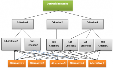
The development of hierarchical structure of hierarchical process is one of the important components that facilitates the analysis of complex problems, as the problem is structured to form a pyramid of multiple levels that includes the overall goal, factors, sub-factors and alternatives by development of problem diagram [7]. Figure 2 clarify the structure of hierarchical process that consist of four levels, level (1) represent the goal or optimal alternative, level (2) represent the main factors, level (3) represent sub-factors, and the level (4) represent the alternatives.
Figure 2. Hierarchical structure Naji [11]
5.2 Pairwise comparisons
AHP technique enabled decision-makers to make pairwise comparisons of importance between decisions elements with respect to the scale describe in Table 2.
For example, comparing objective i and objective j (where i was assumed to be at least as important asj), gave a value a ij as shown in the same table. “Saaty has shown that we can use the entier numbers 1 through 9 to represent approximately the homogenies element comparisons, to indicate smaller differences, decimals are added to these numbers.”
Table 2. Saaty’s fundamental scale Saaty [6]
|
Comparative importance |
Description |
|
1 |
Equally important |
|
3 |
Moderate importance |
|
5 |
Strong importance |
|
7 |
Very strong important |
|
9 |
Extreme important |
|
2,4,6,8 |
Intermediate values |
5.3 Composition
This step starts after the development of the pairwise comparison matrix where the priority of each elements that were compared with each other as substitutes can be determined based on the factors. The mathematical procedure required to complete the fitting includes calculating the eigenvalues and eigenvectors. Eigenvectors mean relative weights, that is, the degree of relative importance of an element among a group of elements. The installation steps for the first level, which includes comparisons of alternatives according to each factor, as follows [7, 10]:
Determine the geometric mean (GM) for each pairwise comparison by Eq. (1):
$G M_{i}=\sqrt[n]{a_{11} * a_{12} * a_{1 n}}$ (1)
where:
GMi: Geometric mean of first raw.
n: No. of criteria or alternatives.
a1n: Element of matrix.
Determine the relative importance or priority by apply Eq. (2):
$R I_{i}=G M_{i} / \sum G M_{i}$ (2)
where:
RIi: Relative importance or priority of first raw, i=1, 2.n.
5.4 Consistency
Consistency indicates to the validity of the judgments made by the decision makers involved in the decision-making process, and these judgments are represented by preferential binary comparisons of alternatives and factors in the AHP. Although the literary writings divided the application steps into three stages, the researcher decided to separate the installation step from stability instead of merging them into one step due to the importance of this step.
In many cases, it is difficult for the decision maker to estimate the correct weights for alternatives, as it is expected that binary comparisons are subject to random error. Therefore, AHP technique allows a certain range of instability and provides a measurement for this case and for each set of judgments, as Saaty found it difficult to find complete and continuous stability.
The reason for the lack of consistency in judgments is due to a lack of information that the individual possesses, a lack of focus during the decision-making process, written errors, or a defect in the structuring of the model for the problem. Therefore, when the order of the matrix is greater than 2 i.e. n ≥ 2 the Consistency Ratio must be extracted for each binary comparisons matrix. The stability of the decision-maker’s comparisons at the first level is checked as follows [10]:
1. Determine (ƛmax) by using Eq. (3):
ƛmax$=\sum \boldsymbol{R} \boldsymbol{I}_{\boldsymbol{i}} * \boldsymbol{W} \boldsymbol{j}$ (3)
where:
RIi: Relative importance of first raw.
Wj: Sum of RI in each column.
2. Determine the constancy index (CI) using Eq. (4):
CI=ƛmax-n/(n-1) (4)
where:
CI: Consistency index.
n: No. of factors or alternatives.
3. Determine consistency ratio (CR) using Eq. (5):
$C R=C I / R C$ (5)
where:
CR: Consistency ratio.
RC: Random consistency it will determine by Table 3:
Table 3. Random index to test the consistency
|
N |
RC |
|
1 |
0 |
|
2 |
0 |
|
3 |
0.58 |
|
4 |
0.90 |
|
5 |
1.12 |
|
6 |
1.24 |
|
7 |
1.32 |
|
8 |
1.41 |
|
9 |
1.45 |
Finally, after ensuring the stability of all matrices, the Synthesis of priority is implemented by calculating the total score for each Si alternative by taking all the vectors for the criteria alternatives and the criteria vectors as follows:
$\boldsymbol{S i}=\sum w i \boldsymbol{RI} \boldsymbol{i} \boldsymbol{j}$ (6)
where:
Si: Priority, i=1, 2… N.
RIij: The relative importance of alternative i and factor j.
Wi: Relative importance of factor j.
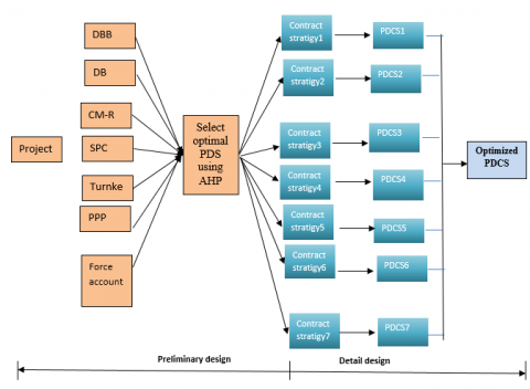
The researcher regards DBB, DB, CM-R, SPC, Turnkey, PPP and force account as the seven fundamental PDS according to the environmental work of wastewater project in Wasit governorate. The researcher proposed that the design process of PDCS can be similar to that of an engineering structure, which usually includes the conceptual design, preliminary design, and detailed design. Accordingly, the PDCS design is divided into two stages, namely, preliminary design and detailed design. During the preliminary design, the optimal PDS will be selected by AHP technique as the framework or template for the next stage, detailed design, in which PDS will be optimized for a wastewater project, and the PDS will be combined together with contract strategy and formed into different options that can be selected. A general design model is clarified in Figure 3.
Figure 3. General design model (researcher)
6.1 Preliminary design
The major task of the preliminary design is to determine which of PDS will be selected, namely, (DB or DB or CM-R or SPC or turnkey or PPP or force account), and one of them will be selected based on main and sub factors that effect on select PDS on wastewater projects, using AHP technique.
6.1.1 AHP model results
Close questionnaire form No. (2) Clarify in Appendix, aim to extent interrelations in the AHP. According to the questionnaire, 10 experts’ knowledge and information in Iraqi construction sector. As a result, AHP can developed as a decision-making provision means. Figure 4 shows the academic certification for the second sample questionnaire of the experts.
Figure 4. Academic certification
The years of experience for the second questionnaire form illustrated in the Figure 5, and we note that more than half of the respondents have more than 20 years of experience.
Figure 5. No. of experience years
The workplace of second questionnaire sample illustrated in Figure 6, we note that respondent from government institutions which has the main role in decisions making in choosing the projects delivery system.
Figure 6. Workplace
Figure 7 clarify the scientific background of for the second questionnaire sample, include many disciplines such as civil, mechanical, and electrical engineering.
Figure 7. Responder’s specialization
The next step of AHP it’s create a pairwise comparison between main factors, as shown in Table 4:
By apply Eq. (1) and Eq. (2) for each row, it will determine the geometric mean (GM) and relative importance as shown in Table 7:
Geometric Mean $(\mathrm{GM})=\sqrt[n]{\mathrm{a}_{11} * \mathrm{a}_{12} * \mathrm{a}_{1 \mathrm{n}}}$
For example: $(\mathrm{GM})=\sqrt[4]{1 * 3 * 9 * 5}=3.409$
RI = GM / total GM, for example: RI = 3.409/6.132 = 0.556.
Table 4. Pairwise comparison between main factors
|
Main factors |
P.O |
O.R |
E.C |
A.A |
GM |
RI |
|
P.O |
1 |
3 |
9 |
5 |
3.409 |
0.556 |
|
O.R |
1/3 |
1 |
8 |
5 |
1.911 |
0.312 |
|
E.C |
1/9 |
1/8 |
1 |
5 |
0.513 |
0.084 |
|
A.A |
1/5 |
1/5 |
1/5 |
1 |
0.299 |
0.049 |
|
Total |
1.644 |
4.325 |
18.2 |
16 |
6.132 |
- |
By apply Eqns. (3), (4) and (5) it will determine the (ƛmax, CI and CR) respectively:
ƛmax =$=\sum R I$*total column
ƛmax= 0.556*1.644 + 0.312*4.325+0.084*18.2+0.049*16 = 4.576
CI= (ƛ_max-n)/ (n-1), CI= (4.576-4)/ (4-1) = 0.192
CR= CI/ RC, CR=0.192/0.90 = 0.213
And Eqns. (1) and (2) will determine the (GM) and (RI) as shown in Table 5:
Table 5. Pairwise comparison between sub factors under P.O
|
P.O |
Q.L |
P.V |
C.P.T |
D.P.C |
V.C |
GM |
RI |
|
Q.L |
1 |
4 |
5 |
5 |
8 |
3.807 |
0.525 |
|
P.V |
1/4 |
1 |
1/2 |
1 |
1/3 |
0.529 |
0.073 |
|
C.P.T |
1/5 |
2 |
1 |
5 |
1 |
1.149 |
0.158 |
|
D.P.C |
1/5 |
1/5 |
1/5 |
1 |
1/4 |
0.684 |
0.094 |
|
V.C |
1/8 |
3 |
1 |
4 |
1 |
1.084 |
0.149 |
|
Total |
1.775 |
10.2 |
7.7 |
16 |
10.58 |
7.253 |
|
ƛmax= 5.973, CI= 5.973-5/5-1 = 0.243, CR=CI/RC= 0.243/1.12=0.22
By apply Eqns. (1) and (2) it will determine the (GM) and (RI) respectively as shown in Table 6:
Table 6. Pairwise comparison between sub factors under O.R
|
O.R |
D.C |
R |
M.T.T |
GM |
RI |
|
D.C |
1 |
1/5 |
1/5 |
0.342 |
0.091 |
|
R |
5 |
1 |
1 |
1.71 |
0.455 |
|
M.T.T |
5 |
1 |
1 |
1.71 |
0.455 |
|
Total |
11 |
2.2 |
2.2 |
3.762 |
|
By apply Eqns. (3), (4) and (5), it will determine (ƛmax, CI, and CR) respectively:
ƛmax= 3.003, CI= 3.003-3/ 3-1 = 0.0015
CR= 0.0015/0.58=0.0025
Eqns. (1) and (2) will determine the (GM) and (RI) respectively as shown in Table 7:
Table 7. Pairwise comparison between sub-factors under E.C
|
E.C |
F.R |
U.M |
C.R.C |
GM |
RI |
|
F.R |
1 |
9 |
3 |
2.999 |
0.594 |
|
U.M |
1/9 |
1 |
1/9 |
0.605 |
0.119 |
|
C.R.C |
1/3 |
9 |
1 |
1.442 |
0.286 |
|
Total |
1.444 |
19 |
4.111 |
5.046 |
|
By apply Eqns. (3), (4) and (5), it will determine (ƛmax, CI, and CR) respectively:
ƛmax=4.29, CI=4.29-3/3-1=0.647, CR= 0.647/0.58 = 1.116
Eqns. (1) and (2), will determine the (GM) and (RI) respectively as shown in Table 8:
Table 8. Pairwise comparison between sub-factors under A.A
|
O.R |
A.S.Q |
S.S.M |
D.C.W |
GM |
RI |
|
A.S.Q |
1 |
3 |
9 |
2.999 |
0.655 |
|
S.S.M |
1/3 |
1 |
7 |
1.326 |
0.289 |
|
D.C.W |
1/9 |
1/7 |
1 |
0.251 |
0.054 |
|
Total |
1.444 |
4.143 |
17 |
4.576 |
|
By apply Eqns. (3), (4) and (5), it will determine (ƛmax, CI, and CR) respectively: ƛmax= 3.061, CI= 0.031, CR= 0.052
Eqns. (1) and (2), will determine the (GM) and (RI) respectively as shown in Table 9:
Table 9. Pairwise comparison between delivery systems under P.O
|
P.O |
DBB |
DB |
CM-R |
SPC |
T |
PPP |
F.A |
GM |
RI |
|
DBB |
1 |
1/7 |
7 |
3 |
1/5 |
7 |
7 |
1.622 |
0.157 |
|
DB |
7 |
1 |
9 |
9 |
3 |
5 |
7 |
4.817 |
0.467 |
|
CM-R |
1/7 |
1/9 |
1 |
7 |
9 |
7 |
3 |
1.546 |
0.15 |
|
SPC |
1/3 |
1/9 |
1/7 |
1 |
5 |
7 |
7 |
1.038 |
0.101 |
|
T |
5 |
1/3 |
1/9 |
1/5 |
1 |
1 |
1/3 |
0.533 |
0.052 |
|
PPP |
1/7 |
1/5 |
1/7 |
1/7 |
1 |
1 |
1/7 |
0.261 |
0.025 |
|
F.A |
1/7 |
1/7 |
1/3 |
1/7 |
3 |
7 |
1 |
0.489 |
0.047 |
|
Total |
13.76 |
2.04 |
17.73 |
20.49 |
22.2 |
35 |
25.48 |
10.306 |
|
By apply Eqns. (3), (4) and (5), it will determine (ƛmax, CI, and CR) respectively:
ƛmax= 11.07, CI= 0.678, CR=0.51
Eqns. (1) and (2), will determine the (GM) and (RI) respectively as shown in Table 10:
Table 10. Pairwise comparison between delivery systems under O.R
|
O.R |
DBB |
DB |
CM-R |
SPC |
T |
PPP |
F.A |
GM |
RI |
|
DBB |
1 |
1/9 |
1/7 |
7 |
1/7 |
5 |
1/3 |
0.594 |
0.05 |
|
DB |
9 |
1 |
5 |
9 |
3 |
9 |
3 |
4.424 |
0.38 |
|
CM-R |
7 |
1/5 |
1 |
7 |
1/5 |
5 |
5 |
1.745 |
0.15 |
|
SPC |
1/7 |
1/9 |
1/7 |
1 |
1/9 |
1 |
1/7 |
0.231 |
0.01 |
|
T |
7 |
1/3 |
5 |
9 |
1 |
9 |
3 |
3.117 |
0.26 |
|
PPP |
1/5 |
1/5 |
1/5 |
1 |
1/9 |
1 |
1/7 |
0.277 |
0.02 |
|
F.A |
3 |
1/3 |
1/5 |
7 |
1/3 |
7 |
1 |
1.184 |
0.1 |
|
Total |
27.34 |
2.28 |
11.68 |
41 |
4.89 |
37 |
12.61 |
11.572 |
|
By apply Eqns. (3), (4) and (5), it will determine (ƛmax, CI, and CR) respectively:
ƛmax= 7.66, CI=0.111, CR=0.084
Eqns. (1) and (2), will determine the (GM) and (RI) respectively as shown in Table 11:
Table 11. Pairwise comparison between delivery systems under E.C
|
E.C |
DBB |
DB |
CM-R |
SPC |
T |
PPP |
F.A |
GM |
RI |
|
DBB |
1 |
1/9 |
1/7 |
5 |
1/9 |
1/9 |
1/9 |
0.271 |
0.02 |
|
DB |
9 |
1 |
1 |
7 |
1 |
7 |
1/7 |
1.808 |
0.17 |
|
CM-R |
7 |
1 |
1 |
7 |
1/9 |
1/7 |
7 |
1.274 |
0.12 |
|
SPC |
1/5 |
1/7 |
1/7 |
1 |
1/9 |
1/9 |
1/5 |
0.192 |
0.02 |
|
T |
9 |
1 |
9 |
9 |
1 |
5 |
9 |
4.424 |
0.40 |
|
PPP |
9 |
1/7 |
7 |
9 |
1/5 |
1 |
9 |
2.039 |
0.19 |
|
F.A |
9 |
7 |
1/7 |
5 |
1/9 |
1/9 |
1 |
0.919 |
0.08 |
|
Total |
44.2 |
10.39 |
18.43 |
43 |
2.64 |
13.48 |
26.45 |
10.927 |
|
By apply Eqns. (4- 3), (4-4) and (4-5), it will determine (ƛmax, CI, and CR) respectively:
ƛmax=11.455, CI=0.74, CR= 0.563
Eqns. (1) and (2), will determine the (GM) and (RI) respectively as shown in Table 12:
Table 12. Pairwise comparison between delivery systems under A.A
|
A.A |
DBB |
DB |
CM-R |
SPC |
T |
PPP |
Force account |
GM |
RI |
|
DBB |
1 |
1/9 |
1/7 |
9 |
1/9 |
1/7 |
1/7 |
0.317 |
0.02 |
|
DB |
9 |
1 |
9 |
9 |
1/3 |
3 |
3 |
3 |
0.26 |
|
CM-R |
7 |
1/9 |
1 |
3 |
1/7 |
1/7 |
1/7 |
0.489 |
0.04 |
|
SPC |
1/9 |
1/9 |
1/3 |
1 |
1/7 |
1 |
1/5 |
0.274 |
0.02 |
|
Turnkey |
9 |
3 |
7 |
7 |
1 |
7 |
7 |
4.876 |
0.42 |
|
PPP |
7 |
1/3 |
7 |
1 |
1/7 |
1 |
1/7 |
0.855 |
0.07 |
|
Force account |
7 |
1/3 |
7 |
5 |
1/7 |
7 |
1 |
1.876 |
0.16 |
|
Total |
40.11 |
5 |
31.5 |
35 |
2.02 |
19.28 |
11.62 |
11.687 |
|
By apply Eqns. (3), (4) and (5), it will determine (ƛmax, CI, and CR) respectively as shown:
ƛmax=8.1194, CI= 0.186, CR=0.141
The final step is to prepare a matrix, this matrix consists of 7 alternatives (delivery systems) in the columns, and 4 main factors in the rows as shown in Table 13. The RI adopted for each factor and each alternative, and then the researcher applied Eq. (6) in order to select the optimal delivery system (optimal alternative).
Table 13. Delivery systems and main factors
|
|
DBB |
DB |
CM-R |
SPC |
T |
PPP |
F.A |
RI |
|
P.O |
0.157 |
0.467 |
0.15 |
0.101 |
0.052 |
0.025 |
0.047 |
0.556 |
|
O.R |
0.05 |
0.38 |
0.15 |
0.01 |
0.26 |
0.02 |
0.1 |
0.312 |
|
E.C |
0.02 |
0.17 |
0.12 |
0.02 |
0.4 |
0.19 |
0.08 |
0.084 |
|
A.A |
0.02 |
0.26 |
0.04 |
0.02 |
0.42 |
0.07 |
0.16 |
0.049 |
By apply Eq. (6), it will determine the optimal PDS as shown in Table 14.
Table 14. Optimal PDS
|
|
DBB |
DB |
CM-R |
SPC |
T |
PPP |
F.A |
RI |
|
P.O |
0.157 |
0.467 |
0.15 |
0.101 |
0.052 |
0.025 |
0.047 |
0.556 |
|
O.R |
0.05 |
0.38 |
0.15 |
0.01 |
0.26 |
0.02 |
0.1 |
0.312 |
|
E.C |
0.02 |
0.17 |
0.12 |
0.02 |
0.4 |
0.19 |
0.08 |
0.084 |
|
A.A |
0.02 |
0.26 |
0.04 |
0.02 |
0.42 |
0.07 |
0.16 |
0.049 |
|
Priority (Si) |
0.104 |
0.405 |
0.142 |
0.062 |
0.16 |
0.039 |
0.072 |
|
The researcher concluded from the results the optimal project delivery system is a design-build (DB), that take maximum priority as (0.405), and the stage of preliminary design has been done, then will be started and start the next step it known (detail design).
6.2 Detailed design
The detailed design is based on the result of the preliminary design. In the detailed design stage, the optimal PDS will matching in contract strategies, the contract strategy should be include (lump sum, unit price, cost plus affixed fee, guaranteed max price and target price incentive contract) then a decision should be made to choose the best one (optimized PDCS). The researcher depends on Likert scale to analyze and compute the arithmetic mean (AM), Table 15 describe the 4-point Likert scale.
Table 15. Four-point Likert scale
|
Interval |
Deference |
Description |
|
1.00-1.74 |
0.74 |
Not suited (N.S) |
|
1.75-2.49 |
0.74 |
Not often use (N.O) |
|
2.50-3.24 |
0.74 |
Fairly suited (F.S) |
|
3.25- 4.00 |
0.75 |
Well suited (W.S) |
The researcher collect and analyze the data that clarify in appendix form NO.10, using SPSS V.20 to measure the suitability of each contract with delivery system, as follow.
6.2.1 DBB and Contract Strategy (PDCS1)
Table 16 clarify the DBB and type of contracts the result shows, the unit price contract is well suited by (AM=3.5), then lump sum and cost plus a fixed fee are fairly suited by (AM= 2.9 and 3) respectively, while guaranteed max price and target price incentive contract it’s not suite.
Table 16. PDCS1
|
Details |
Lump sum |
Unit price |
Cost plus affixed fee |
guaranteed max price |
target price incentive contract |
|
N (valid) |
10 |
10 |
10 |
10 |
10 |
|
N (missing) |
0 |
0 |
0 |
0 |
0 |
|
mean |
2.90 |
3.50 |
3.00 |
1.70 |
1.60 |
|
St. deviation |
.568 |
.707 |
.667 |
.483 |
.516 |
Table 17. PDCS2
|
Details |
Lump sum |
Unit price |
Cost plus affixed fee |
guaranteed max price |
target price incentive contract |
|
N (valid) |
10 |
10 |
10 |
10 |
10 |
|
N(missing) |
0 |
0 |
0 |
0 |
0 |
|
Mean |
2.00 |
1.70 |
2.90 |
3.00 |
3.40 |
|
St. Deviation |
.667 |
.823 |
.568 |
.667 |
.843 |
Table 18. PDCS3
|
Details |
Lump sum |
Unit price |
Cost plus affixed fee |
guaranteed max price |
target price incentive contract |
|
N(valid) |
10 |
10 |
10 |
10 |
10 |
|
N(missing) |
0 |
0 |
0 |
0 |
0 |
|
Mean |
2.00 |
1.60 |
3.00 |
3.20 |
3.30 |
|
St. Deviation |
.667 |
.699 |
.667 |
.632 |
.823 |
|
variance |
.444 |
.489 |
.444 |
.400 |
.678 |
Table 19. PDCS4
|
Details |
Lump sum |
Unit price |
Cost plus affixed fee |
guaranteed max price |
target price incentive contract |
|
N(valid) |
10 |
10 |
10 |
10 |
10 |
|
N(missing) |
0 |
0 |
0 |
0 |
0 |
|
Mean |
2.00 |
3.50 |
3.00 |
2.10 |
2.10 |
|
St. Deviation |
.667 |
.707 |
.667 |
.568 |
.738 |
Table 20. PDCS5
|
Details |
Lump sum |
Unit price |
Cost plus affixed fee |
guaranteed max price |
target price incentive contract |
|
N(valid) |
10 |
10 |
10 |
10 |
10 |
|
N(missing) |
0 |
0 |
0 |
0 |
0 |
|
Mean |
2.20 |
1.30 |
3.00 |
3.00 |
3.70 |
|
St. Deviation |
.632 |
.483 |
.667 |
.667 |
.483 |
Table 21. PDCS6
|
Details |
Lump sum |
Unit price |
Cost plus affixed fee |
guaranteed max price |
target price incentive contract |
|
N(valid) |
10 |
10 |
10 |
10 |
10 |
|
N(missing) |
0 |
0 |
0 |
0 |
0 |
|
Mean |
2.00 |
1.50 |
1.70 |
3.50 |
2.40 |
|
St. Deviation |
.667 |
.707 |
.823 |
.707 |
.516 |
Table 22. PDCS7
|
Details |
Lump sum |
Unit price |
Cost plus affixed fee |
guaranteed max price |
target price incentive contract |
|
N(valid) |
10 |
10 |
10 |
10 |
10 |
|
N(missing) |
0 |
0 |
0 |
0 |
0 |
|
Mean |
2.00 |
2.90 |
3.00 |
1.60 |
3.40 |
|
St. Deviation |
.667 |
.738 |
.667 |
.843 |
.843 |
Table 23. Matching matrix of PDS and CS
|
PDS |
Types of Contracts |
||||
|
Lump sum |
Unit price |
Cost plus a fixed fee |
Guaranteed maximum price (GMP) |
Target price incentive contract |
|
|
DBB |
F.S |
W.S |
F.S |
N.S |
N.S |
|
DB |
N.O |
N.S |
F.S |
F.S |
W.S |
|
CM-R |
N.O |
N.S |
F.S |
F.S |
W.S |
|
SPC |
N.O |
W.S |
F.S |
N.O |
N.O |
|
T |
N.O |
N.S |
F.S |
F.S |
W.S |
|
PPP |
N.O |
N.S |
N.S |
W.S |
N.O |
|
F.A |
N.O |
F.S |
F.S |
N.S |
W.S |
|
Note: DBB = design-bid-build; DB= design-build; CM-R= construction management; SPC =separate prime contracts; T= turnkey; PPP = public privet partnership; F.A=force account |
|||||
6.2.2 DB and Contract Strategy (PDCS2)
The result shows target price incentive contract is well suited in design build delivery system by (AM= 3.4) then guaranteed max price and cost plus are fairly suited but unit price and lump sum are not often use, as shown in Table 17.
6.2.3 CM-R and contract strategy (PDCS3)
The construction manager at risk delivery system is adequate with target price incentive contract by (AM= 3.3) but guaranteed max price and cost plus is fairly suited by (AM=3.2 and 3) respectively, while the lump sum is not often use finally the unit price is not suited by (AM=1.6) as shown Table 18.
6.2.4 SPC and Contract Strategy (PDCS4)
According to the result in Table 19 the separate prime contract (SPC) is well suited with unit price contract by (AM=3.5) also the cost plus fee is fairly suited and each of lump sum guaranteed max price, target price are not often used by (AM=2.00 and 2.10) respectively.
6.2.5 Turnkey and Contract Strategy (PDCS5)
Table 20 shows the turnkey and contract strategy, the result analysis specify that target price incentive contract is well suited by AM=3.7 while cost plus a fixed fee and guaranteed max price are fairly suited by AM=3, and lump sum is not often use, then the unit price not suited.
6.2.6 PPP and Contract Strategy (PDCS6)
The result shows the guaranteed max price is a well suited with the public privet partnership by AM=3.5, while target price incentive contract and lump sum are not often use by AM= 2.4 and 2 respectively, then unit price and cost plus a fixed fee are not suited in this type of PDS, as shown Table 21.
6.2.7 Force Account and Contract Strategy (PDCS7)
Table 22 shows the force account and type of contracts, and the output indicate the target price incentive contract is well suited by AM=3.4, while cost plus and unit price are fairly suited by AM (3 and 2.9) respectively, then lump sum is not often use by AM = 2, finally the guaranteed max price is not suited.
According to the results above the researcher can be create a matching matrix between all projects delivery systems and all types of contracts, in order to select optimal PDCS in wastewater projects, this matrix describe in Table 23.
Seven basic delivery methods for wastewater projects were identified which are DB, DBB, CM, SPC, T, PPP and F.A. and the relative importance of each of the factors adopted in choosing the optimal delivery system was determined and evaluated using pairwise comparison. The influencing factors were divided into main factors and sub factors according to the relative importance. The main factors are the objectives of the project, owner requirements, and the external conditions. And the sub-factors are the level of quality, the size of the project, the completion of the project within the specified period, the degree of complexity of the project. The relative importance of each delivery system was also evaluated within each of the factors adopted in the evaluation and selection of the optimal delivery system. The researcher was able to create a matching matrix between all project delivery systems and all types of contracts suitable for them in order to choose the optimal PDCS for wastewater projects. The result shows that the most appropriate delivery method for wastewater projects is the design built (DB) method, implementation of DB, and that the target price incentive contract is quite suitable for DB by (AM= 3.4), then the guaranteed maximum price and the additional cost are appropriate to some extent, but the unit price and the total amount are not used in many times.
This research represents the researcher's point of view in terms of the factors that have been studied and identified through a questionnaire and a review of previous studies. But there may be factors that have not been discussed that researchers may address in future studies.
|
P.O |
Project objectives |
|
O.R |
Owner requirements |
|
E.C |
External condition |
|
A.A |
Administration aspects |
|
Q.L |
Quality level |
|
P.V |
Project volume |
|
C.P.T |
Complete project in specific time |
|
D.P.C |
Degree of project complex |
|
V.C |
Variance in cost |
|
GM |
Geometric mean |
|
RI |
Relative importance |
|
D.C |
Disputes and claims |
|
R |
Risk |
|
M.T.T |
Modern tools and techniques |
|
F.R |
Finance references |
|
U.M |
Unstable market state |
|
C.R.C |
Contractor resources and capabilities |
|
A.S.Q |
Administration staff and qualification |
|
S.S.M |
Safety and security management |
|
D.C.W |
Difficult of current work |
|
DBB |
Design bid built |
|
DB |
Design built |
|
CM-R |
Construction manager at risk |
|
SPC |
Separated prime contract |
|
T |
Turnkey |
|
PPP |
Privet public partnership |
|
F.A |
Force account |
|
PDS |
Project delivery system |
|
CS |
Contract strategy |
[1] Gordon, C.M. (1994). Choosing appropriate construction contracting method. Journal of Construction Engineering and Management, 120(1): 196-210. https://doi.org/10.1061/(ASCE)0733-9364(1994)120:1(196)
[2] Molenaar, K.R., Songer, A.D., Barash, M. (1997). An automated prediction tool for design-build projects. In Construction Congress V: Managing Engineered Construction in Expanding Global Markets, pp. 582-589.
[3] Spink, C.M. (2014). Choosing the right delivery system. In: Proceedings of the 1997 ASCE Construction Conference, pp. 663-671.
[4] Saaty, T.L. (1996). Multicriteria decision making: The analytic hierarchy process. RWS Publ.
[5] Ibbs, W., Chih, Y.Y. (2011). Alternative methods for choosing an appropriate project delivery system (PDS). Facilities, 29(13/14): 527-541. https://doi.org/10.1108/02632771111178418
[6] Saaty, T.L. (1995). Transport planning with multiple criteria: the analytic hierarchy process applications and progress review. Journal of Advanced Transportation, 29(1): 81-126. https://doi.org/10.1002/atr.5670290109
[7] Jankowski, P. (1995). Integrating geographical information systems and multiple criteria decision-making methods. International journal of Geographical Information Systems, 9(3): 251-273. https://doi.org/10.1080/02693799508902036
[8] Winston, G.C. (1999). Subsidies, hierarchy and peers: The awkward economics of higher education. Journal of Economic Perspectives, 13(1): 13-36. https://doi.org/10.1257/jep.13.1.13
[9] Tam, M.C., Tummala, V.R. (2001). An application of the AHP in vendor selection of a telecommunications system. Omega, 29(2): 171-182. https://doi.org/10.1016/S0305-0483(00)00039-6
[10] Janic, M., Reggiani, A. (2002). An application of the multiple criteria decision making (MCDM) analysis to the selection of a new hub airport. European Journal of Transport and Infrastructure Research.
[11] Naji, H.A. (2006). Building integration model between risk management and value engineering for predicting of construction projects costs, thesis. University of Technology.