Adedayo F. Adedotun* | Olanrewaju K. Onasanya | Abass I. Taiwo | Olumide S. Adesina | Oluwole A. Odetunmibi | Onuche G. Odekina
© 2022 IIETA. This article is published by IIETA and is licensed under the CC BY 4.0 license (http://creativecommons.org/licenses/by/4.0/).
OPEN ACCESS
The use of hard drugs (Alcohol, cocaine and Nicotine) has remained the censorious issue globally and in Nigeria. The use of hard drugs and tobacco smoking is common in the stage of adolescence and youth life, which is a deterrent to education and career advancement. Hence, this study looks into socio-demographic factors that influence the use of hard drugs and tobacco smoking among teenagers between the ages of 15 years to 19 years. To achieve this objective, a cross-sectional data was used and a secondary data was obtained from DHS - National Demographic and Health Surveys (NDHS) from the survey year 2018. Some Bayesian models were developed and Conditional Autoregressive (CAR) model with random walk 1 (RW1) was the best model. The study unveiled a positive significant association of settlement, previous place of residence, education attainment, religion, ethnicity, literacy with reported use of hard drugs amongst teenagers of reproductive age.
Bayesian, spatial model, hard drugs, CAR models, random walk
There has been a significant increase in the use of drugs and the habit of smoking globally and in Nigeria in recent times [1]. Drug use refer to the unlawful use of drugs such as Hallucinogens, barbiturates, heroin, amphetamines, cannabis, opioids and - codeine and cocaine and these have been since as one of the most health, socio–economic and maturity challenges across reproductive ages in the universe and this, in turn, will lead to specific problems and obstacles for addicts, the people or community, and respective families [2-4]. There have been some sex discrepancies in the use of drugs and smoking in society and the fare at which the use of the drug among reproductive teenage men has been noteworthy excessively higher than reproductive teenage women and at that, this breach has continuously declined [5].
Recent studies show clearly that the male and female gender between the ages ten (10) to twenty-nine (39) years or above are involved in the use of drugs [6]. The study showed that it was pronounced between ages 25 and 39. There are high chances of having commercial sex hawkers known as “Prostitute” and shortened as (CSW), law coercion or enforcement consortium, business drivers and some vehicle park scalpers within ages outlined [7-9]. In the light of this, this study investigates the hard drug among Nigerian youths across all states in Nigeria.
In Nigeria, drug use such as cocaine, nicotine and alcohol and smoking are highly prevalent among reproductive and this is due to reasons of sharing of borders with Cameroon, Benin republic [10]. According to World Health Organization, Nigeria is ranked one of the highest intakes of drug and smoking habits in the universe. Drug intake and smoking among Nigerians is almost 2 times the universe average. The 2018 survey from United Nations showed that about 20 million Nigerians use drugs illegally or unlawfully constituting about 3.9% of the world's population users of drug intake [11].
Statistics relating to drug use (cocaine, nicotine and alcohol) and smoking in Nigeria show that approximately 14.4% of the population in Nigeria in the middle of 18 to 54 years of age had been in the use of drugs and smoking but ignoring tobacco and alcohol in the year 2017. Abuse of drugs among Nigerian teenagers' is so rampant, drugs such as opioids (pharmaceutical opioids - codeine, tramadol, and morphine) and amphetamines (methamphetamine and amphetamine). Poly-drug use is also common in the extensive population of Nigeria and also in high users of the drug; details can be found in ref. [11]. The following Table 1 describes the Annual prevalence of drug use in Nigeria among the population 15-54 years of age, 2017.
According to the geopolitical zone, the extent of drug use among teenagers of reproductive age is described as follows; Nigeria which belongs to the continent of Africa comprises six (6) geo-political zones and 37 directorial states. The following are the geopolitical zones - North-Central, South-West, North-East, South-South, North-West, and South-East. According to ref. [11] survey on the research of drug intake in Nigeria, the survey unveiled that southwest zone had a higher previous year chance of drug use than southern geopolitical zones (the gap between 13.8% to 22.4%) in comparison with the Northern geopolitical zones (the gap between 10% to 13.6%). The report also gathered that this increase in the chance of drug use in the southern geopolitical zones is propelled in essence by Lagos and also Oyo states. Varieties of scientific notepaper, as well as published in the peer-reviewed, well-ordered review have shown a good alliance between odds of drug intake and spirituality or religiosity i.e., elevated religious collaboration, religion annexing and religion operation have been widely correlated with slighter use of tobacco, alcohol and further drugs in distinct cultural surroundings. But similarly, scientific writings have also presented that developed areas and various features of the developed societies, including aggregate collective successes such as population density, built society and poverty–stricken neighborhood, possibly correlated with drug use or intake. But in the case of Nigeria, the fact still remains unclear on how unrelated culture, religious authority, social and urbanization impress drug use or intake among the extensive population inside these varieties of geopolitical zones.
Table 1 highlights the use of hard drugs among teenagers of reproductive age according to geopolitical zones in Nigeria:
In comparison with other countries, Nigerian teenagers do not have prevalence on the use of soft drugs such as DMT – “Dimethytryptamine”, Mescaline, LSD – lysergic acid diethylamide and Psiloocylin as compared with hard drugs (Alcohol, cocaine and Nicotine) accross all the states in Nigeria.
Smoking is one of the major causes of avoidable demise and disease or ailment, which is been associated with an elevated burden of chronic unhelpful pulmonary diseases also called (COPD), lung cancer, heart diseases, and partial or chronic stroke [12-14]. Smoking has given a record of over seven million deaths in a year with around ten percent of this follows from severe stroke [15]. Approximately, there are 1.1 billion smokers in the universe and out of this figure; eight percent of them live in middle countries and low-income countries where an extra $\frac{2}{3}$ of smoking associated death happened [15].
Nigeria, the most populous in Africa takes the prime of selling tobacco in the Africa market, having sold at least 18billion tobacco (cigarettes) yearly, and fetching citizens of Nigeria the value of $931 million [15, 16]. Based on WHO conventional program in 2003 on tobacco standards, Nigeria confirms the convention concord in the year 2005, and in that year, Nigeria signed into law for this board to hold (National Tobacco Control) act which is major or primarily to balance all tobacco sway or standards which includes smoking free regions, packaging and advertisement [15]. Despite this advantage, the chance of smoking in Nigeria rises to about 4% in a year [16]. 13 million smokers were estimated in Nigeria in the year 2012 [12], causing sixteen thousand deaths allotted to smoking [17]. Cosmopolitan tobacco establishment has increased tobacco trade and the most important character they played in the growth of nations’ economy may have resulted in the rise of smoking [18, 19]. Though, some federal or public estimates of smoking chance have been announced or described [20, 21], for example, some studies have reported the chance of smoking to be between 3.4% and 17.1% in Nigeria [18] and while the chance of smoking among teenagers is approximately 9% and a mean lifetime of smoking chance of seven percent (7%) to forty-two percent (42%) [16]. The fact remains that the approximate number of smokers is still being debated, which in turn hamper health blueprints. The great concern for this contemporary guess includes poor study plan, representatives of samples and diversities of case definitions.
Table 1. Use of hard drugs (Alcohol, cocaine and Nicotine) among teenagers of reproductive age according to geopolitical zones in Nigeria
|
Annual prevalence of drug use by drug type in North-Central zone |
||||
|
Drug type/Class |
Estimated Prevalence |
Low estimate |
High estimate |
Estimate numbers |
|
Benue |
8.0 |
7.7 |
8.0 |
236,000 |
|
Kogi |
9.2 |
8.9 |
9.2 |
212,000 |
|
Kwara |
13.0 |
12.7 |
13.0 |
213,000 |
|
Nasarawa |
11.8 |
11.4 |
11.8 |
152,000 |
|
Niger |
11.6 |
11.2 |
11.6 |
330,000 |
|
Plateau |
11.0 |
10.8 |
11.1 |
240,000 |
|
FCT (Abuja) |
10.0 |
9.7 |
1 |
180,000 |
|
Annual prevalence of drug use by drug type in North-East zone |
||||
|
Adamawa |
17.0 |
17.0 |
17.0 |
370,000 |
|
Bauchi |
16.0 |
16.0 |
16.0 |
530,000 |
|
Borno |
12.0 |
11.0 |
12.0 |
350,000 |
|
Gombe |
21.2 |
20.7 |
21.2 |
350,000 |
|
Taraba |
14.0 |
13.0 |
14.0 |
213,000 |
|
Yobe |
18.0 |
18.0 |
18 |
300,000 |
|
Annual prevalence of drug use by drug type in North -West zone |
||||
|
Jigawa |
7.0 |
6.8 |
7.0 |
211,000 |
|
Kaduna |
10.0 |
10.6 |
10.0 |
462,000 |
|
Kano |
16.0 |
15.6 |
16.0 |
1,070,000 |
|
Kastina |
12.0 |
11.6 |
12.0 |
481,000 |
|
Kebbi |
12.6 |
12.2 |
12.6 |
286,000 |
|
Sokoto |
9.0 |
8.7 |
9.0 |
230,000 |
|
Zamfara |
13.5 |
13.1 |
13.5 |
312,000 |
|
Annual prevalence of drug use by drug type in South – East Central zone |
||||
|
Abia |
11.3 |
11.0 |
11.3 |
216,000 |
|
Anambra |
1.2 |
10.9 |
11.2 |
317,000 |
|
Ebonyi |
12.8 |
12.4 |
12.8 |
188,000 |
|
Enugu |
16.3 |
15.9 |
16.3 |
370,000 |
|
Imo |
18.1 |
17.7 |
18.1 |
500,000 |
|
Annual prevalence of drug use by drug type in South - West zone |
||||
|
Ekiti |
11.9 |
11.6 |
11.9 |
200,000 |
|
Lagos |
33.0 |
32.0 |
33.0 |
2,117,000 |
|
Ogun |
17.0 |
16.0 |
17.0 |
440,000 |
|
Ondo |
17.0 |
17.0 |
17.0 |
401,000 |
|
Osun |
14.0 |
14.0 |
14.0 |
336,000 |
|
Oyo |
23.0 |
23.0 |
23 |
930,000 |
|
Annual prevalence of drug use by drug type in South-South zone |
||||
|
Akwa – Ibom |
12.5 |
12.2 |
12.5 |
352,000 |
|
Bayelsa |
14.0 |
14.0 |
14.0 |
163,000 |
|
Cross River |
11.8 |
10.4 |
11.8 |
233,000 |
|
Delta |
18.0 |
17.0 |
18.0 |
513,000 |
|
Edo |
15.0 |
15.0 |
15.0 |
330,000 |
|
Rivers |
15.0 |
15.0 |
15.0 |
580,000 |
Source: (United Nations, Department of Economic and Social Affairs, Population Division).
All the aforementioned background information gathered on this study focuses on the prevalence of the use of hard drugs and smoking of tobacco across all states in Nigeria and the prevalence of smoking in Nigeria as a whole but without considering the fact of what are the factors that could lead to the use of hard drugs among citizens of Nigeria from the angle of Bayesian inference. Hence, this research is in pursuance of finding the socio-demographic factors that influence smoking and the use of hard drugs among teenagers of reproductive age between 15-19 years from a parametric Bayesian technique called Bayesian Spatial Model (Bayesian spatial logistic regression) and addressing this question – what is or are the residual geographical residuals at the plain levels? The essence of using this model is to capture the association between these socio-demographic features and the influence of smoking, use of hard drugs and also to model the non – linear effects of the control variables while we give the record of the spatial correlation at plain levels. The findings of this study will assist the national tobacco council which was established by the federal government from the result of WHO congress in 2005 in readjusting their rules and regulations guiding the use or the abuse of hard drugs and tobacco as well. It will also serve as an insight to many researchers on the look for different outcome diversity based on the same topic.
The rest of the paper is presented thus: Section 2 is the literature review, while material and methods are in Section 3, theory and calculations is in section 4, result and discussion is in section 5 and conclusion is section 5. At the end of the paper are the lists of references and an appendix.
Much transnational research has highlighted some selected socio-demographic factors that could associate with the use of hard drugs and smoking or in a nutshell, the use of psychoactive substances, for example in a country like Finland, where a coast to coast survey was carried out on the adult populace by using a self-questionnaire; Kotunla [22] unveiled that by comparing his own country with other European countries, the use of drug and smoking habit among the Finns is less chance to occur but there was a high chance of plenty use of drugs and smoking habit among the population was understudied. In the United States of America, a survey was conducted and reports showed that almost thirty-seven (37%) of the residents use one or something greater than one drug in their days and while in the past twelve months, only 13% had used hard drugs plus in addition with smoking and also before the report was presented, only six (6%) had used them in the month. The report also includes that, for the aged twelve to twenty-five (12-25) years, only sixty – six (66%) had used one of the psychoactive drugs such as cannabis, India-hemps and other drugs, and more excess of 15% of all United States residents aged than eighteen years of age have had some curious solidity use problems. Some reports of the use of hard drugs in the United States of America can be found in the study by Jaffe [23].
In North Africa, popular drug use is cannabis and this is very common and it serves as the traditional drug for members of the Sufi sect but in the East side of Africa, the most common drug used is called the “Khat” as this drug is a culture drug and which is taken among their religious leaders. Similarly, an inflated occurrence of the use of Khat had been revealed also in the life of school teachers, university lecturers and parents as well and other echelon places in the region. In the southern part of Africa, cannabis is widely well informed and used [24].
A nationwide study on adults in five of the geo-political zones in Nigeria shows that the chance of use of tobaccos and cannabis was estimated to be 17% and 3% respectively. Nevertheless, the report was restricted to self–report evaluation of the use of hard drugs among the interviewee [25].
According to Adeyemi and Adeponle [8], and Ahmed [26] adults over the ages of 31 years shows that the joint use of cannabis with alcohol is higher than the joint use of amphetamines and cannabis.
In Nigeria, the following studies relating to students and the use of psychoactive drugs. It was reported that the chance of the use of hard drugs is high [27, 28]. The occurred use of hard drugs among students in higher institutions is salicylate analgesics, constituting 78% and the drug that follows is alcohol, constituting 42% and cigarettes accounted for 11% [29]. In support of the result of [29], varieties of studies have confirmed that the prevalence use of drugs among the students' population is high [30-32]. In the Southern part of Nigeria, a study on the prevalence of drug use among secondary schools was reported to be 24% for tobacco and 65% for alcohol intake and the report also identified that the usage of cannabis, benzodiazepines and amphetamines were all less familiar in the southern part.
A great effort and contribution from many authors on the prevalence of the use of hard drugs and tobacco smoking are highly appreciated and remembered forever. Well, all the aforementioned authors- didn’t consider the fact of the factors that resulted in to use of hard drugs and smoking and hence, this research fills the gap, by applying the Bayesian spatial class model to critically examine the factors that result in to use of hard drugs and smoking and also defining the geographical residual variation at different levels of the control variables identified [33].
3.1 Study design
The study relied on the secondary data obtained from National Demographic and Health Surveys (NDHS) for the survey year 2018. Now a total of one thousand four hundred and sixty-one (1461) teenagers of reproductive age between the age of 15 years to 19. The data includes the socio-demographic description and use of smoking and drug intake data (cocaine, nicotine and alcohol) as our classification drugs. At the administrative states, Nigeria has 36 states and one federal capital territory and the total number of local governments is 774 LGAs in total and six (6) geopolitical zones. The six (6) geopolitical zones examine the spatial variation of the use of hard drugs (cocaine, nicotine and alcohol) and smoking. Software by Team [34] was used for the analysis, the package “rgdal” in R by Bivand et. al. [35] was used to determine the nature of the shapefile of geopolitical zones and while package "ggplot2" by Wickham [36] was in usage to give rise to the maps after following the regression examination.
3.2 Controlled variable
The response variables used in this research are the use of drugs (Alcohol, cocaine and Nicotine) and smoking and which was gotten from the many questions such as: “Have you used illicit drug?” and the result is coded 0 = “No” and 1 = “yes”. And for smoking; the question asked was: “Do you smoke?” and the response was also coded as “Yes” or “No”.
3.3 Control variables
The control variables considered in this research were identified from the literature and they are as follows: age, sex, occupation of respondents' parents, level of respondents' parents' education, level of respondents' parent smoking, age of first abuse, number of siblings in the family, respondents' perception about drug, upbringing, level of initiation, respondent types of place of residence, respondents' childhood place of residence, respondents' region of the previous residence, highest education level, religion, education in a single year, ethnicity, education attainment, literacy, participation of literacy program outside primary, frequency of listening to the radio, frequency of watching television, owns a mobile telephone, sex of the respondent and state of the respondents.
The first diagnostics test on the dataset is to carry out mutlicollinearity test among the control variables by using the generalized variance inflation factor (GVIF) which is the generalization of variance inflation factor called (VIF). The essence of GVIF is to capture the collinearity among the control variables and these include the dummy regressors from many categorical variables all in all the size of the confidence region for associated coefficients. In creative writing, reporting the generalized variance inflation factor raised to the power of half the degree of freedom i.e. $G V I F^{{\frac{1}{2}} d f}$ and where df signifies the degree of freedom for the number of dummy variables in categorical variable corresponds to the $\sqrt{V I F}$, which is applicable for only single coefficient. Based on the rule of thumb, a variance inflation factor of the value 2.5 is a conviction for logistic regression [37].
Preceding inspection on the use of drugs and smoking are majorly based on logistic regression without considering the fact or taking record of geographical groups. Now if the residual or errors obtained from the regression model are unconventional or independent but not spatially correlated, then the model can be fit by using the long run or the generalized additive mixed model. So in this research study, teenagers of reproductive age inhabiting in closest regions were similarly unmeasured and as they are exposed to the social environment, so we hope that there might exist a spatial correlation over different geopolitical zones. The research employed the use of Integrated Nested Laplace Approximation (INLA) Bayesian methodology which has been the most principal option to capture spatial correlation. An alternative but not efficient to capture spatial correlation is the use of Monte Carlo Bayesian method. So to assess the prospective spatial dependence of the use of drugs and smoking, we applied the INLA Bayesian method using the 74 distribution to serve as district of the geopolitical zones to constitute the area unit called the strata. Using the definition of the convolution random – effect model which constitute two random effect term, independent and unstructured random effect $h_{k}$ set aside for each district k and a spatial structured random effect $b_{k}$. The INLA is modeled as a conditional auto- regression for each district, borrowing information from nearby neighbors to result in more efficient values beyond all the districts. The essence of considering a neighborhood shape is that they will both share boundaries with each other. The spatial logistics regression model is modeled as:
$\operatorname{logit}\left(p_{i k}\right)=Z_{i k}^{T} \beta+S\left(t_{i k}\right)+\varphi\left(t_{i k}^{\prime}\right)+b_{k}+h_{k}$ (1)
where, $p_{i k}$ means the probability of the use of hard drugs and same again for smoking for the $i^{t h}$ individual inhabiting in district k, is the structured matrix from the fixed effects control variables, β stands for the vector of regression coefficients, $t_{i k}$ simply denotes the age of teenagers of reproductive age at time and $t_{i k}^{\prime}$ denotes the age of teenagers of reproductive age at first cohabitation for the $i^{t h}$ individual inhabiting in district k.
Following a random walk (RW) which is used prior for the age of teenagers at survey time $S\left(t_{i j}\right)$ is described also. The random walk earlier defined for the teenager’s age of cohabitation $\varphi\left(t_{i j}^{\prime}\right)$ is also defined. For clarity of annotation, let $s_{t}$ means $s\left(t_{i j}\right)$. Random walk of 1st order is then modeled as undisclosed smooth function of the $j^{t h}$ echelon estimate of t in ascending sequence, then $t_{j}, j=1,2,3, \ldots J$. Then we assume that:
$p\left(s_{t 1}\right) \propto$ const (2)
$\left(s_{t j} \mid s_{t_{j-1}}\right) \sim \operatorname{Normal} \cdot\left(s_{t_{j-1}}, \tau_{s}\right)$
$j=1,2,3, \ldots, J$ (3)
For (RW2) i.e. random walk of second order, we presume that:
$p\left(s_{t_{1}}\right)=p\left(s_{t_{1}}\right) \cdot \propto$ const (4)
$\left(s_{t j} \mid s_{t_{j-1}}, s_{t_{j-2}}\right) \sim \operatorname{Normal} \cdot\left(2 s_{t_{j-1}}-s_{t_{j-2}}, \tau_{s}\right)$
$j=3,4, \ldots, J$ (5)
Now where $\tau_{s}$ is called the precision parameter and is known as the inverse of variance parameter. The lofty the precision, the smoother the guess parameter. We assume at default, the logGamma prior distribution is presumed on the log. Of the precision and this is equal to Gamma prior on the precision. This means that $\operatorname{Gamma}\left(c_{1}, c_{2}\right)$, having mean of $\frac{c_{1}}{c_{2}}$ and its variance $\frac{c_{1}}{{c^{2}}_2}$. In this study, we set the prior value of INLA as $c_{1}=1$ and $c_{2}=10^{-6}$. The option of setting $c_{1}=1$ is for the shape parameter of Gamma distribution to minimize this prior to an exponential distribution. The value of $c_{2}$ simply means that the prior precision tends to a large variance and mean.
CAR prior distribution on the shape of spatial random effect is being used to capture the spatial dependence and it is defined as
$\left(b_{k} \mid b_{k \prime_{j}}\right) \sim N O R M A L\left(\bar{b}_{k}, \sigma_{b}{ }^{2} \mid m_{k}\right)$ (6)
$\bar{b}_{k}$ simply denotes the mean of the spatial random effects of the locale or the neighborhood, and $m_{k}$ simply denotes the no. of districts k. We modeled the $h_{k}$ i.e. the spatial unstructured random effect, which is identically and independently normally distributed with mean of 0 and variance of $\sigma_{k}^{2}$. The essence of drawing up spatial model is to allow us, at the same to estimate or guess the residual spatial dependence and check its influence on series of controlled variables related to use of hard drugs and smoking. The interpretation of random effect is that: it shows the effect of the district of residence on the use of hard drugs and smoking on each teenager of reproductive age.
The precision prior $\tau_{b}=1 / \sigma_{b}^{2}$ and $\tau_{h}=1 / \sigma_{h}^{2}$ are allotted to Gamma prior i.e., $\operatorname{Gamma}\left(1,10^{-5}\right)$ and while a hazy prior for $\beta \sim \operatorname{Normal}\left(0,10^{6}\right)$ was assigned. We also selected a non – instructive prior for the boundary and the variance components, which accepts the consideration data to have the substantial affection on the posterior distribution having not been affected by the program of the priors.
The study used the R package and version R.3.5.0, R 3.5.3 to perform all the analysis. The package R-INLA gives a reliable estimate or guesses by a slow computation time to describe the spatial model from the view of Bayesian points. Each respondent has a survey weight which was provided by NDHS to report for the different likelihood nonresponse and selection.
To ascertain that our findings are truly emblematic of the Nigerian population, each sample weight were integrated into the analysis by setting out the option "weight" as our sampling weight in the R function (inla) which scales the log- likelihood of individual and sampling weight [38]. It is important to note that, the sampling weight increases as the individual likelihood function increases.
In the selection of the model, we first included all the control variables in the model, and then choose the best covariance structure among models without considering the district levels random effect, and which is denoted as "NO". The model with only independent and identical random effect $\left(h_{k}\right)$ with lone $C A R\left(b_{i}\right)$ was also considered and the model with both IID random effect and $C A R\left(b_{i}\right)$ is $\left(b_{i}+h_{k}\right)$. Now, once a covariance structure is established, a backward model selection was done in essence of selecting the best put covariance structure. In addition, all the controlled variables were tested for important interchanges. In the regression analysis, any individual variable with missing data points in the selected covariates is removed.
The WAIC [39] was used for model selection criterion. The WAIC is consistent for parameterization and so good for singleton models and is defined as:
$W A I C=p D+L P D$ (7)
where, pD is called the guess effective number of parameters and LPD is called the long run log pointwise predictive density [40]. Models having a smaller value of WAIC are chosen because they are the best combination of meanness and fitness. A model with WAIC within 2 units of the best model have the same model and a model with a large WAIC have a worse model fit [40].
5.1 Descriptive analysis of variables studies
Table 2 shows that 80.2% of teenagers of reproductive age are well concentrated in the rural areas than in the urban areas constituting only 19.8%.
Table 3 shows that across each geopolitical zones, North West is more spread than any other geopolitical zones, having a higher concentration of teenagers of reproductive age 38.8%, and then followed by North East 27.7%. The least spread zone is the South West having a proportion of 3.5% (of teenagers of reproductive age).
Table 4 shows that, out of 1171 teenagers of reproductive age that settles in the rural areas, only 577 used hard drugs constituting 49.3%, while in the urban areas, only 143 out of 290 used hard drugs. But reverse is in the case of teenagers of reproductive age that smokes in both rural and urban areas. The table above indicates that, out of 1171 teenagers, 1170 do not smokes in the rural areas meaning that in all the rural areas, teenagers do not smoke or simply the chance or the likelihood of smoking among teenagers of reproductive age is slim or critically low. Similarly, in the urban residence, all teenagers in the area do not smoke at all i.e., the chance of this occurrence (smoking among urban areas) is zero.
From the research, 172 teenagers of reproductive age that lived in the countryside "do use" hard drugs as compared with 204 teenagers of reproductive age that do not use hard drugs but also lived in the countryside. The odd ratio is reported to be 0.84 $\left(\frac{172}{204}\right)$ meaning that teenagers of reproductive age that lived in the countryside and do use hard drugs is 0.84 times the number of teenagers that do not use hard drugs. Similarly, 376 teenagers of reproductive age do not smoke at all in comparison with teenagers that have settled in a large city, towns and not smoking as well. This connotes that teenager of reproductive age that do not smoke are concentrated in the countryside.
Table 5 revealed that; mostly male and female teenagers of reproductive age were born in the year 1999 as compared with same-gender following other years of births. These male and female teenagers of reproductive age are averagely 19 years of old and reside mostly in the rural areas of Northwest geopolitical zones of Nigeria possessing a "no education".
Table 2. Frequency distribution of teenagers across the rural and urban residence
|
Stratification by residence |
Frequency |
% |
|
Rural |
1171 |
80.20 |
|
Urban |
290 |
19.80 |
|
Total |
1461 |
100.0 |
Table 3. Frequency distribution of teenagers across the geopolitical zones
|
Stratification by Geopolitical Zones |
Frequency |
% |
|
North Central |
226 |
15.5% |
|
North East |
404 |
27.7% |
|
North West |
567 |
38.8% |
|
South East |
94 |
6.4% |
|
South-South |
118 |
8.1% |
|
South West |
52 |
3.5% |
|
Total |
1461 |
100.0 |
5.2 Collinearity test among the controlled variables under studies
Mutlicollinearity test was so important to test to know the actual variables to be needed in the Bayesian model to build. Table 6 above presents the multicollinearity test on the control variables studied. The table reveals that Respondent parents’ education, Respondent parents’ smoking/use of drug, Number of siblings and Respondent perception were all in concern because the $G V I F^{\frac{1}{2(V I F)}}$ values of these controlled variables are greater than 2.5 which is beyond the rule of thumb. Hence the variables are deleted and are not given further concern.
Table 4. Descriptive statistics of demographic characteristics of smoking and use of hard drugs among teenagers of reproductive age in Nigeria
|
Controlled variables |
Use of Drug |
Smoke cigarettes |
|||
|
Yes |
No |
Yes |
No |
||
|
According to residence |
Rural |
577 |
594 |
1 |
1170 |
|
Urban |
143 |
147 |
0 |
290 |
|
|
Type of place of previous residence (rtpr) |
Capital |
- |
- |
|
- |
|
Large city |
- |
- |
- |
- |
|
|
City |
32 |
26 |
- |
58 |
|
|
Town |
68 |
51 |
- |
119 |
|
|
Country side |
172 |
204 |
- |
376 |
|
|
Abroad |
- |
- |
- |
- |
|
|
Highest level of Education |
No education |
411 |
427 |
1 |
837 |
|
Primary |
84 |
103 |
- |
187 |
|
|
Secondary |
224 |
208 |
- |
432 |
|
|
Tertiary |
1 |
3 |
- |
4 |
|
|
Religion |
Catholic |
47 |
35 |
- |
82 |
|
Other Christian |
157 |
159 |
- |
316 |
|
|
Islam |
510 |
540 |
1 |
1049 |
|
|
Traditionalist |
1 |
1 |
- |
2 |
|
|
Other |
5 |
6 |
- |
11 |
|
|
Ethnicity |
Ekoi |
3 |
4 |
- |
7 |
|
Fulani |
92 |
112 |
- |
204 |
|
|
Hausa |
307 |
312 |
1 |
618 |
|
|
Ibibio |
9 |
15 |
- |
24 |
|
|
Igala |
14 |
11 |
- |
25 |
|
|
Igbo |
54 |
49 |
- |
103 |
|
|
Ijaw |
15 |
22 |
- |
37 |
|
|
Kanuri |
16 |
18 |
- |
34 |
|
|
Tiv |
17 |
17 |
- |
34 |
|
|
Yoruba |
25 |
21 |
- |
46 |
|
|
Other |
168 |
160 |
- |
328 |
|
|
Don’t Know |
- |
- |
- |
- |
|
|
Education Attainment |
No education |
411 |
427 |
1 |
837 |
|
Incomplete primary |
31 |
40 |
- |
71 |
|
|
Complete primary |
53 |
63 |
- |
116 |
|
|
Incomplete secondary |
149 |
127 |
- |
276 |
|
|
Complete secondary |
75 |
81 |
- |
156 |
|
|
Higher |
1 |
3 |
- |
4 |
|
|
Literacy |
Can’t read at all |
510 |
529 |
1 |
|
|
Able to read only part of sentence |
117 |
124 |
- |
1038 |
|
|
Able to read whole sentence |
93 |
88 |
- |
241 |
|
|
No card with required language |
- |
- |
- |
181 |
|
|
Blind/visually impaired |
- |
- |
- |
- |
|
|
Listening to Radio |
Not at all |
453 |
483 |
1 |
935 |
|
Less than once a week |
141 |
129 |
- |
270 |
|
|
At least once a week |
126 |
129 |
- |
255 |
|
|
Almost every day |
- |
- |
- |
- |
|
|
Owns a mobile phone |
No |
492 |
510 |
1 |
1001 |
|
Yes |
228 |
231 |
- |
459 |
|
|
Level of respondents’ parent education |
Primary |
227 |
235 |
- |
462 |
|
Secondary |
254 |
240 |
1 |
493 |
|
|
Tertiary |
239 |
266 |
- |
505 |
|
|
Level of respondents’ parents use of drugs and smoking |
Low |
227 |
235 |
- |
462 |
|
Mild |
254 |
240 |
1 |
493 |
|
|
High |
239 |
266 |
- |
505 |
|
|
Sex of respondents Male Female |
Male |
370 |
368 |
- |
738 |
|
Female |
350 |
373 |
1 |
722 |
|
5.3 Comparison of model selection based on WAIC
The researchers tried various Bayesian model, originally the researchers proposed CAR, CAR + IID, IID - linear models alongside with random walk of order 1 and random walk of order 2 by considering CAR, CAR +IID and IID respectively but later introduced BYM model, LEROUX and SAC model and found out that CAR random effect was the best covariance structure among other Bayesian models because it gave the lowest WAIC value of “9021.23 [12.89]”. The next thing we did is to select the best of the best fixed effect controlled variables once the covariance structure has been defined or found out. These fixed effect control variables were selected using the backward model selection and the following variables were selected level of respondents’ parent education, owns a mobile phone, listening to radio, literacy, education attainment, ethnicity, religion, highest level of education, type of place of previous place of residence and according to residence as control variables as indicated in Table 8 displaying the selected Bayesian model used “CAR”. Now in other to check the aftermath of wrong specifications of district size random effect and also the disorderliness of this variable "current age of the respondents", hence we, therefore, incorporated the selected control variables after model choice and also, we consider modeling the numeric – continuous control variable i.e., the age of the respondent, possessing non – linear effect and linear effect using RW 2 and RW 1.
Table 5. Cross tabulation of sex of respondent across some demographic characteristics
|
Demographic characteristics |
Sex of the respondent |
||
|
Male |
Female |
||
|
Year of respondent born |
1998 |
25 |
25 |
|
1999 |
286 |
274 |
|
|
2000 |
255 |
270 |
|
|
2001 |
134 |
114 |
|
|
2002 |
32 |
30 |
|
|
2003 |
6 |
10 |
|
|
Respondent current age |
15 years |
7 |
11 |
|
16 years |
37 |
32 |
|
|
17 years |
136 |
126 |
|
|
18 years |
274 |
273 |
|
|
19 years |
286 |
281 |
|
|
Geopolitical Zones |
North central |
121 |
105 |
|
North East |
218 |
186 |
|
|
North West |
264 |
303 |
|
|
South East |
50 |
44 |
|
|
South - South |
56 |
62 |
|
|
South West |
29 |
23 |
|
|
Region |
Rural |
586 |
585 |
|
Urban |
152 |
138 |
|
|
Highest level of education |
No education |
407 |
431 |
|
Primary |
100 |
87 |
|
|
secondary |
229 |
203 |
|
|
tertiary |
2 |
2 |
|
Table 6. Generalized variance inflation factor of all control variables
|
Controlled variables |
GVIF |
DF |
$G V I F^{\frac{1}{2(V I F)}}$ |
|
Type of place of residence |
2.099 |
6 |
1.0637 |
|
Type of place of previous residence |
1.673 |
4 |
1.066 |
|
Highest education level |
3.892 |
3 |
1.254 |
|
Religion |
2.762 |
3 |
1.185 |
|
Ethnicity |
1.984 |
5 |
1.071 |
|
Education in single year |
2.563 |
3 |
1.169 |
|
Education attainment |
1.993 |
4 |
1.09 |
|
Literacy |
2.884 |
4 |
1.142 |
|
Ever participated in a literacy program outside primary |
1.466 |
2 |
1.1 |
|
Listening to radio program |
2.102 |
2 |
1.204 |
|
Watching television |
1.984 |
2 |
1.1868 |
|
Owns a mobile phone |
2.002 |
2 |
1.189 |
|
State of resident |
4.847 |
36 |
1.022 |
|
Respondent parents’ education |
1302 |
3 |
3.3044 |
|
Respondent parents’ smoking/use of drug |
1498 |
2 |
6.2213 |
|
Number of siblings |
58290 |
6 |
2.495 |
|
Respondent perception |
9880 |
3 |
4.632 |
Comparison of model selection based on WAIC, which connotes that there exists a "within district" correlation in the use of hard drugs among teenagers of reproductive age in Nigeria according to the population data because the model “NO” yielded a higher value of WAIC as indicated in the bold figure. In the middle of other participated models, now modeling the current age of the teenagers following linear effect performs unpleasantly than the other models despite impressive random walk of order 1 or random walk of order 2. By considering RW 1 for this current age of teenagers of reproductive ages, this model is more preferable to RW 2. In checking across all the models, the CAR + RW 1 model was the best because it yields the smallest WAIC and hence, it is being selected as the final Bayesian method and also the reason for picking is that it will include the spatial structures of all the control variables and predicting the model will be accurate.
Table 7. Comparison of model selection to have a good covariance structure
|
Model studied |
WAIC value obtained |
|
|
Linear effect model |
NO |
11893.58 [120.47] |
|
CAR |
19021.23 [12.89] |
|
|
CAR + IID |
16098.144 [34.78] |
|
|
IID |
13.8938.092 [39.281] |
|
|
RW1 |
NO |
19902.289 [56.188] |
|
CAR |
*10384.53 [11.902]* |
|
|
CAR + IID |
19535.90 [18.18] |
|
|
IID |
19536.28 [198.28] |
|
|
RW2 |
NO |
19027.4732 |
|
CAR |
14753.9029 [19.384] |
|
|
CAR + IID |
16384.28 [89.38] |
|
|
IID |
13026.892 [78.27] |
|
|
OTHER BAYESIAN MODEL INTRODUCED IN “INLA” BAYESIAN METHODS |
||
|
BYM |
18672.29 [234.903] |
|
|
LEROUX |
12936.027 [169.374] |
|
|
SAC |
18647.37 [189.273] |
|
|
SEM |
20546.28 [145.56] |
|
|
SDM |
13930.289 [49.944] |
|
|
SLM |
16974.902 [239.938] |
|
5.4 Factors influencing the use of Hard drugs (Alcohol, cocaine and Nicotine)
The parameter estimates for the CAR, IID and no models with the current age of the teenagers’ reproductive age which is modeled with RW 1 is reported in Table 8. As mentioned in section 6.3, the findings from IID + CAR are absent because IID + CAR model yielded the same result as IID as revealed in the table under section 5.3. Also, this means that the control variable effects of CAR models and IID were all the same and this connotes that at the district level, the estimation or the guess of the control variable is not affected by the correlation edifice or structure of the random effect. Nonetheless, the significant effect of the highest level of education, literacy, education attainment, level of respondents' parent education and religion of the respondents were more conspicuous under the CAR models and IID in juxtaposition to the model minus the district linear random effects, which means model “NO”. Under the model “NO”, the covariate effect – under the model “NO”, both large city and city were highly positively, significantly related with the use of drugs and while in other models like CAR, only capital was positively related with the use of hard drugs. This simply means that there was a significant correlation in the district with the use of hard drugs; this should help to assess the qualities of the controlled variable effects.
Table 8. Odds Ratio (OR) adjustment and its 95% confidence intervals (CI)
|
|
CAR MODEL |
IID MODEL |
NO MODEL |
||||
|
CONTROLLED VARIABLES |
ODD RATIO (OR) |
95% CI |
ODD RATIO (OR) |
95% CI |
ODD RATIO (OR) |
95% CI |
|
|
According to residence |
Rural |
|
|
|
|
|
|
|
Urban |
1.189 |
[0.99, 1.2] |
1.29 |
[0.69, 1.5] |
1.13 |
[0.87, 1.4] |
|
|
Type of place of previous residence (rtpr) |
Capital |
|
|
|
|
|
|
|
Large city |
|
|
1.19 |
[1.99, 1.2] |
2.189 |
[0.79, 2.2] |
|
|
City |
|
|
1.4 |
[2.489, 2.5] |
2.304 |
[0.49, 2.4] |
|
|
Town |
|
|
1.9 |
[1.99, 2.2] |
1.589 |
[0.19, 1.6] |
|
|
Country side |
1.114 |
[0.29, 1.2] |
1.414 |
[1.89, 1.5] |
1.804 |
[0.59, 1.9] |
|
|
abroad |
|
|
1.29 |
[1.89, 1.4] |
1.289 |
[0.89, 1.4] |
|
|
Highest level of Education |
No education |
1.041 |
[0.59, 1.3] |
1.043 |
[0.89, 1.3] |
1.044 |
[0.59, 1.3] |
|
Primary |
|
|
|
|
|
|
|
|
Secondary |
|
|
1.043 |
[0.69, 1.3] |
1.043 |
[0.59, 1.3] |
|
|
tertiary |
|
|
1.299 |
[0.49, 1.5] |
1.292 |
[0.49, 1.5] |
|
|
Religion |
Catholic |
|
|
1.674 |
[0.89, 1.8] |
|
|
|
Other Christian |
2.181 |
[0.79, 2.2] |
2.189 |
[0.79, 2.2] |
2.189 |
[0.79, 2.2] |
|
|
Islam |
2.314 |
[0.43, 2.4] |
2.389 |
[0.40, 2.4] |
2.318 |
[0.43, 2.4] |
|
|
Traditionalist |
|
|
1.582 |
[0.17, 1.6] |
1.532 |
[0.49, 1.6] |
|
|
other |
|
|
1.828 |
[0.56, 1.9] |
1.819 |
[0.69, 1.9] |
|
|
Ethnicity |
Ekoi |
|
|
1.104 |
[0.99, 1.4] |
1.214 |
[0.68, 1.6] |
|
Fulani |
1.289 |
[0.69, 1.2] |
1.219 |
[0.69, 1.5] |
|
|
|
|
Hausa |
3.084 |
[2.39, 3.3] |
|
|
1.214 |
[0.68, 1.6] |
|
|
Ibibio |
1.229 |
[0.99, 1.4] |
1.229 |
[0.69, 1.5] |
1.123 |
[0.87, 1.4] |
|
|
Igala |
1.024 |
[0.49, 1.3] |
1.134 |
|
1.234 |
[0.68, 1.6] |
|
|
Igbo |
1.139 |
[0.69, 1.2] |
1.219 |
[0.69, 1.5] |
|
|
|
|
Ijaw |
|
|
1.114 |
[0.99, 1.4] |
1.24 |
[0.68, 1.6] |
|
|
Kanuri |
|
|
1.29 |
[0.69, 1.5] |
1.13 |
[0.87, 1.4] |
|
|
Tiv |
|
|
|
|
1.24 |
[0.68, 1.6] |
|
|
Yoruba |
|
|
1.29 |
[0.69, 1.5] |
1.13 |
[0.87, 1.4] |
|
|
Other |
|
|
1.114 |
[0.99, 1.4] |
|
|
|
|
Don’t Know |
|
|
|
|
1.13 |
[0.87, 1.4] |
|
|
Education Attainment |
No education |
1.274 |
[0.89, 1.8] |
1.674 |
[0.89, 1.8] |
1.674 |
[0.89, 1.8] |
|
Incomplete primary |
1.392 |
[1.18,1.42] |
|
|
1.19 |
[0.49, 2.1] |
|
|
Complete primary |
|
|
1.304 |
[0.49, 2.4] |
1.314 |
[0.61, 2.2] |
|
|
Incomplete secondary |
1.471 |
[1.2, 1.5] |
2.589 |
[0.19, 2.6] |
|
|
|
|
Complete secondary |
|
|
|
|
0.804 |
[0.22, 1.6] |
|
|
Higher |
|
|
0.289 |
[0.89, 1.4] |
|
|
|
|
Literacy
|
Can’t read at all |
2.289 |
[0.40, 2.4] |
2.381 |
[0.40, 2.4] |
2.356 |
[0.40, 2.4] |
|
Able to read only past of sentence |
|
|
1.582 |
[0.17, 1.6] |
1.502 |
[0.17, 1.6] |
|
|
Able to read whole sentence |
|
|
1.828 |
[0.56, 1.9] |
|
|
|
|
No card with required language |
1.204 |
[0.99, 1.4] |
|
|
1.114 |
[0.99, 1.4] |
|
|
Blind/visually impaired |
|
|
2.389 |
[0.40, 2.4] |
|
|
|
|
Listening to Radio |
Not at all |
1.214 |
[0.68, 1.6] |
1.354 |
[0.68, 1.6] |
2.181 |
[0.79, 2.2] |
|
Less than once a week |
|
|
1.203 |
[0.87, 1.4] |
2.314 |
[0.43, 2.4] |
|
|
At least once a week |
|
|
1.302 |
[0.68, 1.6] |
|
|
|
|
Almost every day |
|
|
1.293 |
[0.87, 1.4] |
1.819 |
[0.56, 1.9] |
|
|
Owns a mobile phone |
No |
0.220 |
[0.08, 0.3] |
1.214 |
[0.68, 1.6] |
1.214 |
[0.68, 1.6] |
|
Yes |
1.123 |
[0.47, 1.4] |
1.123 |
[0.87, 1.4] |
1.123 |
[0.87, 1.4] |
|
|
Level of respondents’ parent education |
Primary |
1.225 |
[1.89, 2.3] |
2.314 |
[0.43, 2.4] |
1.304 |
[0.99, 1.4] |
|
Secondary |
2.219 |
[1.99, 2.4] |
1.582 |
[0.13, 1.6] |
1.229 |
[0.69, 1.5] |
|
|
Tertiary |
1.39 |
[1.07, 2.5] |
1.819 |
[0.56, 1.9] |
1.184 |
[0.99, 1.4] |
|
|
Standard error estimate of random effect(s) |
|||||||
|
$\operatorname{CAR}\left(\sigma_{b}\right)$ |
0.47 |
[0.32, 0.48] |
|
|
|
|
|
|
$\operatorname{IID}\left(\sigma_{h}\right)$ |
|
|
0.27 |
[0.21, 0.38] |
|
|
|
|
Current age of the respondent |
0.17 |
[0.12, 0.39] |
0.26 |
[0.22, 0.32] |
0.19 |
[0.28, 0.39] |
|
Under the model "CAR" and "NO" the controlled effects of "Highest level of education” – No education, primary and secondary and “Ethnicity levels” such as Ekoi, Fulani, Hausa, Ibibio, Igala, Igbo, Ijaw, Kanuri, Tiv and Yoruba all had a less positive relationship on the use of hard drugs but as in the models “CAR, IID and NO”, the covariate effect of Religion - other Christians and Islam gives a high report of positive statistical relationship on the use of drugs. Under the model “CAR” both complete education and attainment of higher education factor is highly positive and significantly related with the use of hard drugs as compared with IID model where only levels – “Incomplete primary” and “Incomplete secondary” are farthest positive related to use of hard drugs. Under the model “CAR, IID and NO” the levels of literacy – “Can’t read at all” is farthest related to the use of hard drugs as compared to other levels of literacy and finally under the model “CAR, IID, NO” the categorical controlled effects – listening to radio, owns a mobile phone have a low or minute positive relationship on the use of hard drugs.
The control variables’ effect estimated based on the best-fitted model CAR, with the current age of the teenagers of reproductive ages, which is model as random walk of order 1, are explained as follows:
5.5 Check of sensitivity Analysis (Re estimating the posterior Mean)
A sensitivity analysis was controlled to check for the peppiness of the Bayesian induction. Now assuming the posterior distribution is dynamic and when the prior parameters are changed then the Bayesian induction or inference is not consistent and dependable. So the research pursued further to make some changes and the following changes are: the parameters $c_{1}=1, c_{2}=10^{-6}$ of Gamma prior for the precision parameter τ was changed to $c_{1}=0.004, c_{2}=10^{-3}$ and then the prior distribution for the precision parameters were changed to so many distributions and these distributions are Penalized complexity known as (PC), Half Cauchy, Half Normal, Half t and Uniform distributions as indicated in Table 9. It is important to note that the estimates for the control variables when the prior specification of the precision parameter was used is the same as when the hyperparameters are changed. Hence for the sake of clarity, their results were not reported.
Table 9. Sensitivity analysis
|
Distribution used |
Mean |
95% CI |
|
|
Half – Cauchy
(WAIC – 12406.34) |
Respondent current age |
0.056 |
[0.05, 0.8] |
|
Respondent year of Birth |
0.089 |
[0.08, 0.10] |
|
|
District (74 district) |
0.012 |
[0.005, 0.05] |
|
|
Half – Normal
|
Respondent current age |
0.17 |
[0.085, 0.3] |
|
Respondent year of Birth |
0.189 |
[0.05, 0.308] |
|
|
District (74 district) |
0.11 |
[0.03, 0.3] |
|
|
Half – t
|
Respondent current age |
0.486 |
[0.15, 0.8] |
|
Respondent year of Birth |
0.228 |
[0.1, 0.3] |
|
|
District (74 district) |
0.192 |
[0.05, 0.4] |
|
|
Uniform |
Respondent current age |
0.14 |
[0.08, 0.2] |
|
Respondent year of Birth |
0.19 |
[0.02, 0.28] |
|
|
District (74 district) |
0.13 |
[0.09, 0.4] |
|
|
Penalized complexity |
Respondent current age |
0.102 |
[0.08, 0.18] |
|
Respondent year of Birth |
0.127 |
[0.07, 0.2] |
|
|
District (74 district) |
0.129 |
[0.08, 0.3] |
|
5.6 Residual Geographical Variation i.e., spatial disparity in Use of Drugs
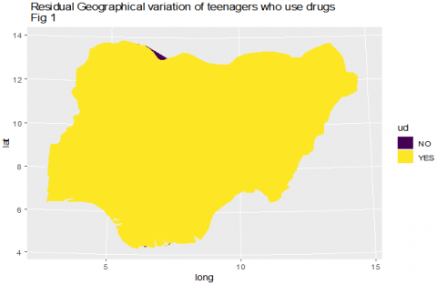
Figure 1 shows the posterior means for the Nigeria districts' random effects from the CAR model fitted as shown in Table 8, which adjusted all the control variables studied. Figure 1 indicates that there is a higher residual concentration in the use of hard drugs among teenagers in all states of Nigeria i.e., no state is left out. All teenagers of reproductive age across all Nigeria geopolitical zones do use hard drugs and it means that no state is widely dispersed more than other states.
Figure 1. Residual geographical variation of teenagers who use drugs
The main objective of the study was to develop a Bayesian method to determine the socio-demographic factors that could influence smoking and the use of hard drugs (Alcohol, cocaine and Nicotine) and find the residual geographical variations or the states with a high concentration on the use of drugs. A cross-sectional data was used and secondary data was obtained from DHS - National Demographic and Health Surveys (NDHS) from the survey year 2018. One thousand four hundred and sixty-one (1461) teenagers of reproductive age were considered between the ages 15 years to 19 years. Different Bayesian models were proposed to capture the socio-demographic factors. It was found out that CAR random effect had the best covariance structure to identify these socio–demographic factors among other Bayesian models because it gave the lowest WAIC value of "9021.23 [12.89]”. Such factors identified from the CAR model after considering the current age of all teenagers of reproductive age which is modeled as random walk 1 (RW1) were areas of concentration – the use of hard drugs did not differ among teenagers that reside in rural and urban areas, and these teenagers are widely spread in the area of settlements such as large city, city and towns and these teenagers that use hard drugs had no education among the northern hemisphere of Nigeria. The study showed that Christian teenagers use more hard drugs than teenagers in Northern Nigeria and other parts of Nigeria.
The study unveiled a positive significant association of settlement areas or residence, previous place of residence, education attainment, the highest level of education, religion, ethnicity, literacy with reporting on the use of hard drugs among teenagers of reproductive age. The identified socio-demographic factors and districts are at an increase in the likelihood of the use of hard drugs and prevention is strictly needed especially education, which is to be shared equally among all teenagers of reproductive age in Nigeria. It is important to conclude that as the age of teenagers is increasing, the use of hard drugs is being reduced. The geographical residual variations on the use of hard drugs are widely spread across Nigeria's geographical zones indicating that about 95% of teenagers of reproductive age do use hard drugs irrespective of their tribes.
The research study investigated unobserved spatial variation in use of hard drugs especially - alcohol, nicotine and cocaine and smoking while studying the impact of a range of socio and demographic factors. Our study accounted for the geographical clustering and flexible modeling the non-linear effects of the continuous covariates for drawing a valid statistical inference, now the question that may arise is: if there is a linear effect in the continous covariates, what best statistical bayesian approach would be preferred as this to serve as the future research direction?
I hereby acknowledge Covenant University Centre for Research, Innovation and Discovery (CUCRID) for their support toward the completion of this research.
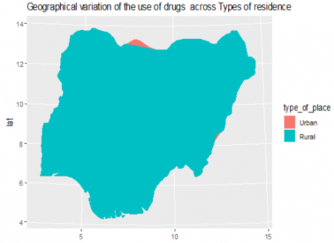
Figure 2. Geographical variation of the use of drugs across types of residence
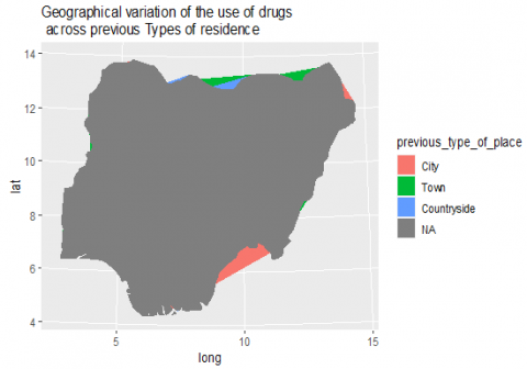
Figure 3. Geographical variation of the use of drugs across previous types of residence
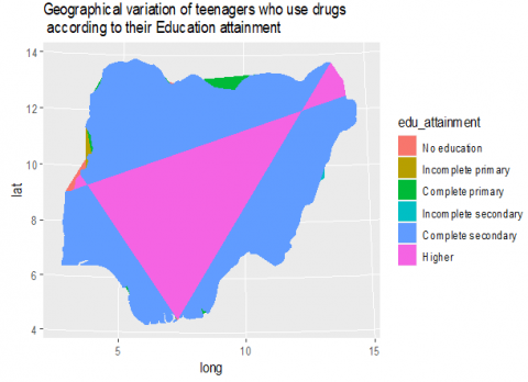
Figure 4. Geographical variation of teenagers who use drugs according to their highest level of education
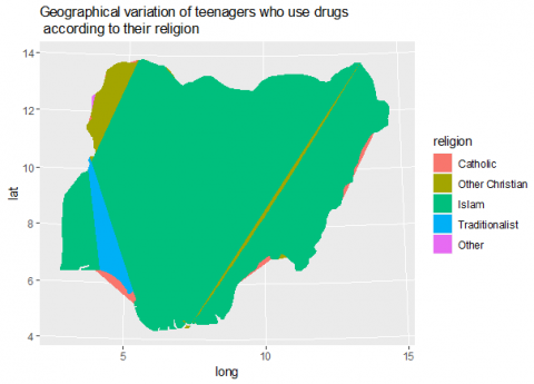
Figure 5. Geographical variation of teenagers who use drugs according to their religion
Figure 6. Geographical variation of teenagers who use drugs according to their education attainment
[1] Adeloye, D., Auta, A., Fawibe, A., et al. (2019). Current prevalence pattern of tobacco smoking in Nigeria: a systematic review and meta-analysis. BMC Public Health, 19, 1719. https://doi.org/10.1186/s12889-019-8010-8
[2] Compton, W.M., Boyle, M., Wargo, E. (2015). Prescription opioid abuse: Problems and responses. Prev Med., 80: 5-9. https://doi.org/10.1016/j.ypmed.2015.04.003
[3] Ahmadpanah, M., Mirzaei-Alavijeh, M., Allahverdipour, H., Jalilian, F., Haghighi, M., Afsar, A., Gharibnavaz, H. (2013). Effectiveness of coping skills education program to reduce craving beliefs among addicts referred to addiction centers in Hamadan: A randomized controlled trial. Iran J Public Health, 42(10): 1139-1144.
[4] Surwani, Akhmetshin, E.M., Okagbue, H.I., Laxmi Lydia, E., Shankar, K. (2020). Digital economic challenges and economic growth in environmental revolution 4.0. Journal of Environmental Treatment Techniques, 8(1): 546-550.
[5] Lal, R., Deb, K.S., Kedia, S. (2015). Substance use in women: Current status and future directions. Indian J Psychiatry, 57(Suppl 2): S275-85. https://doi.org/10.4103/0019-5545.161491
[6] United Nations Office on Drugs and Crime. (2006). page 25.
[7] United Nations Drug Control Programme (2006) Country Profile on Nigeria.www.unodc.org/unodc/undcp, accessed on July 5, 2021.
[8] Adeyemi, G.T., Adeponle, A.B. (2006). An overview of psychoactive substance use and misuse in northern Nigeria. Nigerian Journal of Psychiatry, 4(1): 9-19. https://doi.org/10.4314/njpsyc.v4i1.39884
[9] Gureje, O., Degenhardt, L., Olley, B., Uwakwe, R., Udofia, O., Wakil, A., Adeyemi, O., Bohnert, K.M. and Anthony, J.C. (2007) A descriptive epidemiology of substance use and substance use disorder in Nigeria during the early 21st century. Drug and Alcohol Dependence, 91(1): 1-9. http://dx.doi.org/10.1016/j.drugalcdep.2007.04.010
[10] Adebiyi, A.O., Faseru, B., Sangowawa, A.O., Owoaje, E.T. (2010). Tobacco use amongst out of school adolescents in a local government area in Nigeria. Substance Abuse Treatment, Prevention, and Policy, 5: 24. http://dx.doi.org/10.1186/1747-597X-5-24
[11] United Nations Office on Drugs and Crime. (2018). page 25.
[12] World Health Organization. WHO Report on the Global Tobacco Epidemic, 2019. Geneva: World Health Organization; 2019. https://apps.who.int/iris/bitstream/handle/10665/326043/9789241516204-eng.pdf, accessed on 3 Nov. 2019.
[13] Hecht, S.S. (2003). Tobacco carcinogens, their biomarkers and tobacco-induced cancer. Nat Rev Cancer., 3(10):733. https://doi.org/10.1038/nrc1190
[14] Drope J, Schluger N, Cahn Z, et al. (2018). The Tobacco Atlas. Atlanta: American Cancer Society and Vital Strategies.
[15] World Health Organization. WHO global report on trends in tobacco smoking 2000 –2025. Geneva: World Health Organization; 2015. https://www.who.int/tobacco/publications/surveillance/reportontrendstobaccosmoking/en/, accessed on 21 Jan. 2019.
[16] Ake A. (2018). Nigeria: Tobacco Consumption Contributes 12% Deaths from Heart Diseases - NHF. THISDAY.
[17] The Tobacco Atlas. Nigeria. https://tobaccoatlas.org/country/nigeria/, accessed on 28 Dec. 2018.
[18] Oyewole, B.K., Animasahun, V.J., Chapman, H.J. (2018). Tobacco use in Nigerian youth: A systematic review. PloS One, 13(5): e0196362. https://doi.org/10.1371/journal.pone.0196362
[19] Ibidunni, S., Olawande, T., Olokundun, M., Iruonagbe, C., Adelekan, I. (2019). Diversity issues in Nigeria’s healthcare sector: Implications on organizational commitment. A cross-sectional study. F1000Research, 8: 1-8. https://doi.org/10.12688/f1000research.19350.1
[20] Adeniji, F., Bamgboye, E., van Walbeek, C. (2012). Smoking in Nigeria: Estimates from the Global Adult Tobacco Survey (GATS) 2012. Stroke.
[21] Mbulo, L., Kruger, J., Hsia, J., Yin, S., Salandy, S., Orlan, E.N., Agaku, I., Ribisl, K.M. (2018). Cigarettes point of purchase patterns in 19 low-income and middle-income countries: Global adult tobacco survey, 2008-2012. Tobacco Control, 28(1): 117-120. https://doi.org/10.1136/tobaccocontrol-2017-054180
[22] Kontula, O. (1995). The prevalence of drug use with reference to drug use in Finland. The International Journal of Addictions, 30(8): 1053-1066. https://doi.org/10.3109/10826089509055827
[23] Jaffe, M. (1995) Amphetamine Use in USA. The International Journal of Addiction, 856-990.
[24] ICNB Annual Report. (2004). Vienna, Austria.
[25] Fatoye, F.O., Marakinyo, O. (2002). Substance use among secondary school students in rural urban communities in Southwestern Nigeria. East African Medical Journal, 79(6): 299-305. https://doi.org/10.4314/eamj.v79i6.8849
[26] Ahmed, M.H. (1986). Drug abuse as seen in the university department of psychiatry, Kaduna, Nigeria, in 1980-1984. Acta Psychiatrica Scandinavica, 74(1): 98-101. http://dx.doi.org/10.1111/j.1600-0447.1986.tb06234.x
[27] Lambo, T.A. (1960). Further neuro-psychiatric observation in Nigeria. British Medical Journal, 2: 1696-1714. http://dx.doi.org/10.1136/bmj.2.5214.1696
[28] Asuni, T. (1964). Socio-psychiatric problem of cannabis in Nigeria. U.N. Bulletin on Narcotics, 16: 17-28.
[29] Adelekan, M.L., Abiodun, O.A., Obayan, R.O. (1992) Prevalence and pattern of substance use among undergraduate in a Nigerian University. Drug and Alcohol Dependence, 29(3): 255-261. http://dx.doi.org/10.1016/0376-8716(92)90100-Q
[30] Adelakun, M.L., Odejide, O.A. (1989). The reliability and validity of the WHO student drug use questionnaire among Nigerian Students. Drug and Alcohol Dependence, 24(3): 245-249. http://dx.doi.org/10.1016/0376-8716(89)90062-8
[31] Akinhanmi, O.A. (1996). Drug Abuse among Medical Student in a State University in Nigeria. A Dissertation Submitted to West African College of Physicians.
[32] Ibidunni, S. Abiodun, J., Ibidunni, O., Olokundun, M. (2019). Using explicit knowledge of groups to enhance firm productivity: A data envelopment analysis application. South African Journal of Economic and Management Sciences, 22(1): 1-9 http://dx.doi.org/10.4102/sajems.v22i1.2159
[33] Chinonye, L.M., Olokundun, M., Falola, H., Ibidunni, S., Amaihian, A., Inelo, F. (2016). A review of the challenges militating against women entrepreneurship in developing nations. Mediterranean Journal of Social Sciences MCSER Publishing, Rome-Italy, 7: 64-69. http://doi.org/10.5901/mjss.2016.v7n1p64
[34] Team, R.C. (2020). R: A language and environment for statistical computing. R Foundation for Statistical Computing, Vienna, Austria. https://www.R-project.org/.
[35] Bivand. R, Keitt. T, Rowlingson. B (2021). Package ‘rgdal’, Bindings for the 'Geospatial' Data Abstraction Library.
[36] Wickham. H. ggplot2: Elegant Graphics for Data Analysis. Springer-Verlag New York, 2016.
[37] Fox, J., Monette, G. (1992). Generalized collinearity diagnostics. J Am Stat Assoc., 87(417): 178-183. http://dx.doi.org/10.1080/01621459.1992.10475190
[38] Rue, H., Martino, S., Chopin, N. (2009). Approximate Bayesian inference for latent gaussian models by using integrated nested Laplace approximations. J R Stat Soc Ser B Stat Methodology, 71(2): 319-392. http://dx.doi.org/10.1111/j.1467-9868.2008.00700.x
[39] Watanabe, S. (2010). Asymptotic equivalence of Bayes cross validation and widely applicable information criterion in singular learning theory. J Mach Learn Res., 11: 3571-3594.
[40] Bishop, S.A., Okagbue, H.I., Odukoya, J.A. (2020). Statistical analysis of childhood and early adolescent externalizing behaviors in a middle low-income country. Heliyon, 6(2): e03377. http://dx.doi.org/10.1016/j.heliyon.2020.e03377