Carlos Matovelle
© 2021 IIETA. This article is published by IIETA and is licensed under the CC BY 4.0 license (http://creativecommons.org/licenses/by/4.0/).
OPEN ACCESS
Using models of organic matter degradation and dissolved oxygen consumption, the concentrations of these compounds are analyzed in two stretches of a river after a discharge of raw sewage. The analyzed river has low drafts and widths, so the velocity is high and the aeration coefficient kr calculated with the Covar method is high, this indicates a rapid recovery of oxygen from the water consumed by the organic matter degradation processes, the river has been instrumented to measure flows and organic matter at various points to calibrate the model. The hydraulic parameters of the river section are analyzed in three control points, in each one sample are taken to analyze oxygen consumption by organic matter and nitrification through laboratory tests to determine and adjust the kinetics of the processes (kd; knit). This kinetics have been used in the development of a water quality model to verify its adjustment, obtaining higher RMSE results than with kinetics from secondary sources. It is observed that the river has an excellent capacity for self-purification due to the high income of dissolved oxygen, with a kr > 9 d-1.
water quality, water quality models, water resource, organic matter
The water resource contamination problems have different origins, from natural contamination and the other anthropogenic processes that end up with their wastewater discharged without adequate purification processes. One of the activities that are of particular interest is livestock since its waste contains a high pollutant load with organic matter and fecal matter. Within this problem, mathematical models as an analysis tool of the system have an outstanding contribution to the development of scientific knowledge of specific areas.
Within a body of water, the physical, chemical, and biological variables can change in a short period, even in hours [1], such as the variations of dissolved oxygen between day and night [2], the variations due to the border entries they have greater importance within the analysis of the water body [3], when studying dynamic systems such as Andean rivers due to their flow and the loads of pollutants that enter them, these variations should be considered to evaluate the scenario.
Water quality models can predict and simulate the impact generated by diffuse and point sources of pollutants in a body of water. They are tools for the development of management plans and policies to protect water resources [4]. Mathematical quality models are management tools that will make it possible to understand the behavior and cause-effect of the processes suffered by the receiving environment to evaluate different alternatives [1, 5]. To achieve adequate management and use of the model in an initial phase, it must be calibrated and validated; thus, it can predict the concentration of pollutants for different scenarios [1, 6].
Within the process of calibrating a model, the behavior of the different parameters that simulate the techniques included in it must be considered and, therefore, it is necessary to implement a methodology that guarantees an appropriate calibration of said parameters, which allows the user the detailed study of defined scenarios for the environmental characterization of the stream [5]. In this context, to ensure that the model is as close to reality, it is necessary to work with kinetics that indicates the appropriate process for the area of interest; this is achieved with the experimentation of the behavior of what is to be simulated.
The results may be useful for management decisions [3], but the entire environment within the river to be modeled must be taken into account. In the rivers understudy, land use has been primarily altered by agricultural and livestock activities. The biggest problem with these activities is their contribution to both the point source and the non-point source of pollution, for example, pesticides and nutrients (mainly phosphorus and nitrogen) discharged into water bodies [7, 8], the models of water quality allow to consider all these variables in which data are often not available [3], they are used to address the characteristics of the aquatic landscape that includes complex geomorphology [9], systems in which the boundary conditions are complicated [10] and internal processes [11].
A water quality model uses data on different scales depending on its objectives, and it can use hourly meteorological data, daily flow data, and monthly chemical and biological analysis data [12]. Although the input data are monthly, results are expected from the quality model with high resolutions inclusive per hour [13]. For these reasons, some modelers move towards more complex models such as two and three dimensions [3]. Others believe that the observed data's quality determines the precision of the model and not the complexity [14].
According to Melching and Yoon [15], the surface reaeration coefficient (K2) and the carbonaceous deoxygenation coefficient (Kd), which is the oxygen consumption due to the degradation of organic matter, are the dominant parameters in terms of the reliability of the simulation of dissolved oxygen concentrations. In streams of rivers. If they are determined experimentally, these constants allow reducing the uncertainty generated when using estimated values or adopting assumptions that do not conform to reality [4].
In rivers with Andean characteristics, re-aeration plays a significant role in recovering the aquatic system [16]. Understanding the behavior of Andean rivers in the face of different loads of organic matter due to specific and diffuse discharges will make it possible to guarantee that the action plans that are carried out are appropriate for the environment. This is achieved with the particular knowledge of the rivers of analysis since they present specific characteristics that make their dynamics rise. By having small drafts and high speeds, the coefficient of surface re-aeration is Fly high, allowing plenty of oxygen to enter the water body.
The Andean rivers are under high pressure due to the lack of appropriate sanitation systems, the available information is scarce. Even geochemical data to know the state of the rivers in Ecuador are not enough [17]. In addition to the lack of information, it is observed that the management of water resources directly affects the concentration of dissolved oxygen. The flow of Andean rivers is directly related to the concentration of dissolved oxygen [18], so improperly managing rivers will increase the risk of a loss of oxygen and an increase in the concentration of organic matter that cannot be degraded.
Water quality models have been developed for Andean rivers, particularly for the Cuenca River that is fed by the Yanuncay River, where the pressure that exists on the resource with wastewater discharges with concentrations of organic matter is evidenced [19]. In these models, the parameters of organic matter measured as BDO5 turns out to be a good indicator of contamination in connection with ecological models [20]. Wastewater discharges must be constantly monitored and this data must be applied in tools such as water quality models that allow evidence of the real impact of pollutants, specifically organic matter that can sometimes be eliminated over very long distances [21].
2.1 Description of the study area
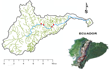
The river studied is the Yanuncay in the Province of Azuay in southern Ecuador; this river is born on the Andes' eastern slope and makes up the upper basin of the Paute River, this is one of the most critical hydrographic basins in the country, with a very high priority for management and conservation. The “Daniel Palacios” dam is located there, where most Ecuador's hydroelectric energy is produced [22].
Livestock activities have been developed in the soils of the sub-basin that have caused deterioration in water quality. The impacts of livestock to the detriment and contamination of water are substantial; these impacts must be seen from a chain perspective that goes from the production of inputs and pastures for animal feed to the transformation of animal products [23], in addition to a large presence of wastewater with high loads of organic matter and coliforms.
In the middle area of the river is the Sustag Drinking Water Treatment Plant, which is one of the monitoring points for calibration of the model and for evaluating the quality of the water being collected. The Yanuncay River is one of the four rivers that the city of Cuenca crosses, so achieving tools that model water quality is of great interest to guarantee the good state of the body of water.
The presence of farms in which specific spills of pollutants are carried out in the area has affected the quality. There are no appropriate management plans to determine the behavior of the resource; for this reason, four monitoring points have been taken (Figure 1), before the discharge, in the release and two control points outside the mixing zone to perform the calibration of the model, the first control point of great importance since it is located in the place of water uptake before a plant of purification.
Figure 1. Location of the study area
With this background, the research focuses on evaluating degradation, nitrification, and reaeration kinetics [24, 25], necessary to carry out the mathematical model for the river and understand the dynamics of pollutants and their effect on the resource.
To evaluate the water quality and the hydrodynamic behavior of the riverbed, monitoring campaigns were carried out for three years, in the periods 2016/2017, 2017/2018, and 2018/2019, according to the guidelines of the World Meteorological Organization, WMO [26]. Each point is coded as presented in Table 1, and samples were taken from them according to the proposed timing, analyzed in the laboratory to determine the kinetics to be tested in the model and the hydrochemical behavior.
Table 1. Sampling points for the determination of kinetics and calibration of the model
|
Code |
Point |
Monitoring frequency (Quality / Flow) |
|
P1 |
Before discharge |
Monthly / daily |
|
P2 |
Wastewater discharge |
Monthly / daily |
|
P3 |
Catchment |
Monthly / daily |
|
P4 |
Calibration point |
Monthly / daily |
The points have been chosen based on conditions of interest, P1 will serve as the “white” point where no water contamination problems have been detected. P2 is a monitoring point for wastewater discharge, it serves as an input parameter for pollutant loads, points P3 and P4 are model calibration points, although P3 is of primary importance because it is located in the catchment. of drinking water, this allows adjusting the model and evaluating the quality of water that reaches this point of interest.
2.2 Determination of hydraulic parameters
Chemical and biological processes are controlled to a high degree by physical phenomena related to the water body's hydrodynamics, which determines the currents and mixing levels that affect the concentration of substances through transport processes. With the hydrological, meteorological, and bathymetric information, the model is adapted to the area of interest, initially obtaining the river's hydrodynamics, which was later used in the simulations of the transport of pollutants [27].
The analyzed river section has a length of 8.35 km from the point P1 before the discharge to the final calibration point of the P4 model (Figure 2). The morphometry of the central area, the dilution sources, abstraction, tributaries to the channel, and the dispersion coefficient are analyzed using the tracer test [28]; at each monitoring point, daily flows are explored through a previous calibration of the expenditure curve. In each of the sections proposed, speed, width, depth, and the longitudinal dispersion coefficient are also measured.
Figure 2. Hydraulic model of the river section
2.3 Degradation rate estimation (kd)
To determine the deoxygenation kinetic constant due to the action of BOD in the receiving stream, the Bosko equation [29] was used, in which the k1 degradation obtained in the laboratory is related to the processes that it undergoes in a natural stream. Such as turbulent mixing, due to the presence of suspended and sedimented organisms, due to the depth of the channel, among other factors [30], Eq. (1) is used to relate these processes:
$k_{d}=k_{1}+n \frac{U}{H}$ (1)
where, k1 is the oxygenation rate obtained in the laboratory through the processing and statistical analysis of each sample, and n U / H represents microorganisms' action in the bed. The coefficient n depends on the analyzed river section's slope and can vary between 0.1 - 0.6.
2.4 Estimation of the reaeration rate (kr)
Reaeration is the process by which oxygen enters from the atmosphere to the water column due to the river's dynamics. The patterns that condition the behavior of this parameter are different from those of degradation, so it is essential to study the parameters that govern this behavior, the solubilization of oxygen is proportional to the difference between saturation oxygen and dissolved oxygen present in the body of water at a given time [24, 31], and it can be represented with Eq. (2):
$\frac{d O_{2}}{d t}=-k_{r} D$ (2)
where, D is the dissolved oxygen deficit in water determined by (Osat - O2).
The entry of oxygen occurs through the air-water interface, where the film is thin. The diffusion of oxygen occurs through the water body slowly, and in turbulent rivers, the re-aeration process is carried out faster [32].
To determine the reaeration kinetics, a variation of the method used by [33] was applied, with a conservative tracer in which the flow rate, time, and concentration of the tracer were determined during the test, each sampling was repeated in the same periods of the water quality intakes and was compared with the Covar method. Also, the micro-basin height and the temperature correction constant are taken into account [16]. There are some equations to calculate the reaeration rate, validated in different rivers with different hydraulic characteristics [19], which have been grouped in the Covar method and are presented in Eqns. (3), (4), (5) [34-36].
$k_{r}=3.93 \frac{U^{0.5}}{H^{1.5}}$ (3)
$k_{r}=5.03 \frac{U^{0.969}}{H^{1.672}}$ (4)
$k_{r}=5.32 \frac{U^{0.67}}{H^{1.85}}$ (5)
where: U = mean flow velocity (m / s); H = mean draft (m).
2.5 Nitrification rate estimation (knit)
Nitrification consists of the transformation of ammoniacal nitrogen into nitrate by implementing a set of nitrifying autotrophic bacteria [37]. This consumption can be validated in the laboratory by determining the biochemical demand for nitrogen-oxygen DBON and in the field by sampling Kjeldahl nitrogen—total (NKT) in each of the analysis sections. Comparisons of the results obtained in the laboratory were made to get DBON through the oxygen consumption test without inhibiting the action of nitrifying bacteria and the stoichiometric relationship DBON = LN = 4.57 * NKT. The constant 4.57 is the stoichiometric factor from the amount of oxygen required to oxidize the total nitrogen in ammonia.
For the first analysis, the equations of the nitrification behavior are obtained in the laboratory test for each of the monitoring points and through an analysis of the flow velocities obtained with the tracer and hydrodynamic tests, Eq. (6):
$L_{N}=L_{N o} e^{-\frac{k_{n i t}}{U} X}$ (6)
where, LNo is the initial DBON for the nitrification model and the variables X and U relate the hydrodynamic characteristics of the analyzed river sections.
2.6 Approach of the water quality model for the river section
The proposed model simulates the pollutants' behavior in the selected river section before the discharge of wastewater. After it, to identify the evolution of the pollutants modeled before a point of interest, that is, the water catchment. BOD5 is modeled as organic load, the consumption of Dissolved Oxygen by the degradation and nitrification processes. The model's resolution and adjustment are made with the experimental kinetics to know its behavior of the river with data obtained in the laboratory.
It is considered a one-dimensional system in length and in which there are no dispersive processes; in this way, the balance equation can be proposed for each pollutant as:
$\frac{\partial L}{\partial t}=-u_{x} \frac{\partial L}{\partial x}-k_{d} \theta^{T-20} \frac{O}{O+\frac{k_{d}}{2}} L-\frac{V S_{L}}{h} L$ (7)
$\frac{\partial\left[\mathrm{O}_{2}\right]}{\partial t}=-u_{x} \frac{\partial\left[\mathrm{O}_{2}\right]}{\partial x}-k_{d}^{\prime}-k_{n i t} L+k_{r}^{\prime}(D)$ (8)
Eqns. (7) and (8) have been simplified, and the convective transport is only found on the x-axis and the processes suffered by the modeled pollutants. This is born from the hypothesis of considering highly convective rivers. For organic matter, the decrease in concentration due to degradation processes has been considered. For dissolved oxygen, the consumption due to the degradation of organic matter, ammonium nitrification, and reaeration is taken into account. This model is intended to be an initial contribution to the management of Andean rivers with experimental kinetic constants, which is why the models are simplified to understand the obtained kinetics' assistance.
For the application, the GESCAL module of the AQUATOOL program was used to determine the evolution of DBOC and dissolved oxygen in the Yanuncay River. The processes considered include the sedimentation and degradation of DBOC, the re-aeration of oxygen, the demand for oxygen from the sediments [38].
In the exploratory analysis of the data at the sampling points in the degradation kinetic variables, it can be observed in Figure 3 that there are atypical values in P1 and P4, this would cause the estimate of the central tendency value to be affected by; therefore, a robust estimator is used (20% trimmed mean), it can also be seen that the variability of the kinetic constants in the three points does not exceed 17%, thus being relatively stable in their behavior.
Significant contrast differences are found in the three points' averages by applying a robust test of variance based on the trimmed mean. The test is used with a confidence level of 95%. The posthoc test shows that there are no similarities between any of the combinations evaluated. Table 2 presents the statistical calculations of mean, median, coefficient of variation, and robust coefficient of variation calculated through medians.
Figure 3. Kinetic outlier analysis
Table 2. Statistical measurements of degradation kinetics
|
Measure |
P1 |
P3 |
P4 |
|
mean |
0.1537000 |
0.7277792 |
0.4061625 |
|
median |
0.15300 |
0.69800 |
0.40045 |
|
cv |
11.28705 |
13.23786 |
16.14197 |
|
cvr |
2.28957 |
21.35032 |
7.13880 |
A CV between 0-30% indicates that the data are few variables based on the classical statistics [39] since the median and the mean do not differ significantly, the central tendency of the data to the median will be taken as a reference because the graph shows atypical data in point 1 and point 4 of sampling. To identify the differences between the mean values of the three sampling points, a contrast test, a parametric ANOVA model, and a robust model based on the contrast of medians are applied. The assumptions for the ANOVA model are verified with a Shapiro-Wilk normality test.
According to the statistical analysis described above, it is concluded that the model cannot be performed with a single value for the degradation kinetics but that it is necessary to use each of those obtained per point of analysis. The water quality model has been constructed so that the kinetic value changes at each end and thus adjusts to the observed data.
A similar statistical process is carried out for the laboratory data of the degradation kinetics and re-aeration, obtaining values for each point without being averaged by their difference. These results are shown in Table 3:
Table 3. Kinetic values for each point
|
Kinetic |
P1 |
P3 |
P4 |
|
kd |
0.15300 |
0.69800 |
0.40045 |
|
kr |
9.5398 |
8.8393 |
9.38932 |
|
knit |
0.0455 |
0.14500 |
0.11393 |
The water quality model has been applied to the section after the discharge of wastewater and after collection, where there are measured data to verify the model's calibration with the application of laboratory kinetics. According to the statistical analysis, the results are presented by section since it is necessary to work with different kinetics for each reach.
A water quality model has to be calibrated [40] to serve as a management tool; generally, it is an iterative process that depends on changing the variables until an adjustment is achieved. In this case, the calibration process will be exclusive with the entry of laboratory kinetics. By calculating the root-mean-square error (RMSE), the model's adjustment is verified for each section and the variables of organic matter and dissolved oxygen.
Figure 4. Results for model calibration with laboratory kinetics
Figure 4 (A) and (B) are the results for the first section analyzing organic matter and dissolved oxygen. For organic matter, the RMSE entered the observed and modeled data with an unadjusted kinetic of 26.15, and in comparison with the kinetics calculated in the RMSE, it is 1.6. For dissolved oxygen, the RMSE between the observed data and the default kinetics and the laboratory kinetics is 0.4 and 0.2, respectively, so it can be analyzed that the model is less sensitive to reaeration kinetics since it is adjusted with a lower percentage of error.
Figure 4 (C) and (D) are the results for the second section; for the organic matter, the RMSE entered the observed and modeled data with kinetics without adjustment is 28.1 and compared with the kinetics calculated in the RMSE is 0.3. For dissolved oxygen, the RMSE between the data observed and the default kinetics and the laboratory kinetics is 0.7 and 0.1, respectively, the behavior coinciding with the previous section analyzed.
The two modeled water quality parameters (BOD and DO) and the two sections of the analyzed river show different behaviors when they are modeled with kinetics available from bibliographic sources and the adjustments with kinetics obtained in the laboratory that present satisfactory values measured with RMSE. The behavior of the BOD is the one that needs the most adjustment (Figure 4. A-C) where the simulated values (theoretical kinetics) differ greatly from the observed data.
The kinetics that is commonly found in reference sources or water quality models made in other countries or a different type of river do not consider the specific dynamics and conditioning factors found in high mountain rivers such as altitude, oxygen saturation, the change in slope, and the mixture of waters with a concentration of organic matter with different biodegradation due to the pressures and discharges that exist on these channels.
In similar research such as [41, 42], mathematical processes applied to each model used are used, achieving adjustments identical to those presented, in this way, it can be verified that obtaining laboratory kinetics adjusts the model to reality and could subsequently be subjected to calibration and mathematical validation process, reducing the uncertainty of the model. On the other hand, in Ecuador, the application of water quality models validated with laboratory data to generate indices is scarce [43]. This type of research allows having an input that can be applied in the development of water quality models surface with greater precision.
Mathematical processes that somehow reduce the error of the simulated data with reality will always have better precision and can be used as a useful tool, within the water quality models we have seen in this research what to add to a conventional calibration process of kinetics an intermediate process through laboratory validations significantly improves the final results and considerably brings them closer to the actual observed results.
In the two sections of the river in which the model was executed, the best adjustments were made using the kinetics of each process obtained in the laboratory. Another critical piece of data is the use of different kinetics for each of the sections, and this allows an adjustment within the general framework of the modeled environmental system. The calibration indicates a robust model with a deficient error that can serve as a management and planning tool adjusted to the area's reality and the biological and physical processes that play a fundamental role in water quality.
This work contributes to understanding the behavior of a river with the characteristics as mentioned above for the Andes when it receives high loads of organic matter and ammonia, whose degradation processes by microorganisms represent a significant consumption of dissolved oxygen in the water and also contribute to scientific knowledge so that the management plans focused on the preservation and guarantee of the water supply for the population are adequate.
The modeling of water quality in Andean rivers is still an issue that has a lot of scientific and technical development ahead, it is expected that in addition to being able to adjust other types of kinetics to the models, greater variables such as the increase in temperature or the flow variability due to climate change, these are processes that are directly related to water quality and it is time to consider qualitative and quantitative models with scenarios of global variations.
This research has been financed by funds from the V contest of the Catholic University of Cuenca's research projects.
|
kd |
kinetics of degradation of organic matter d-1 |
|
k1 |
rate to degradation of organic matter d-1 |
|
n |
slope coefficient |
|
U |
mean flow velocity m. s-1 |
|
H |
mean draft m |
|
kr |
reaeration kinetics d-1 |
|
O2 |
dissolved oxygen in water mg. l-1 |
|
LN |
biochemical nitrogen oxygen demand mg. l-1 |
|
knit |
nitrification kinetics d-1 |
|
X |
reach length |
|
L |
concentration of total organic matter in water mg. l-1 |
|
VSL |
sedimentation rate of particulate organic matter m. s-1 |
|
Greek symbols |
|
|
$\partial \mathrm{L}$ |
organic matter variation |
|
$\partial\left[\mathrm{O}_{2}\right]$ |
dissolved oxygen variation |
|
$\Theta$ |
arrhenius coefficient for temperature |
[1] Chapra, S.C. (2008). Surface Water-Quality Modeling. New York (N.Y.): McGraw-Hill.
[2] Yates, K.K., Dufore, C., Smiley, N., Jackson, C., Halley, R.B. (2007). Diurnal variation of oxygen and carbonate system parameters in Tampa Bay and Florida Bay. Marine Chemistry, 104: 110-124. https://doi.org/10.1016/j.marchem.2006.12.008
[3] Sadeghian, A., Chapra, S.C., Hudson, J., Wheater, H., Lindenschmidt, K. (2018). Improving in-lake water quality modeling using variable chlorophyll a / algal biomass ratios. Environmental Modelling & Software, 101: 73-85. https://doi.org/10.1016/j.envsoft.2017.12.009
[4] Nadal, A., Fortunato, P., Aguirre, S. (2017). Modelación de oxígeno disuelto y DBO5 con tasas cinéticas determinadas experimentalmente: Un aporte para la gestión del arroyo Chicamtoltina. Rev. la Fac. Ciencias Exactas, Físicas y Nat., 4(1): 23.
[5] Arroyave, D., Moreno, A., Toro, F.M., Gallego, D., Carvajal, L.F. (2013). Estudio del modelamiento de la calidad del agua del río Sinú, Colombia. Rev. Ing. Univ. Medellín, 12(22): 57-72.
[6] Cox, B.A. (2003). A review of dissolved oxygen modelling techniques for lowland rivers. Science of The Total Environment, 314-3116: 303-334. https://doi.org/10.1016/S0048-9697(03)00062-7
[7] Chislock, M.F., Doster, E., Zitomer, R.A., Wilson, A.E. (2013). Eutrophicati on: Causes, consequences, and controls in aquati c ecosystems. Nat. Educ. Knowl., 4(4): 1-8.
[8] Wu, Y., Chen, J. (2013). Investigating the effects of point source and nonpoint source pollution on the water quality of the East River ( Dongjiang ) in South China. Ecol. Indic., 32: 294-304. https://doi.org/10.1016/j.ecolind.2013.04.002
[9] Missaghi, S., Hondzo, M. (2010). Evaluation and application of a three-dimensional water quality model in a shallow lake with complex morphometry. Ecol. Modell., 221(11): 1512-1525. https://doi.org/10.1016/j.ecolmodel.2010.02.006
[10] Jin, K., Ji, Z., James, R.T., Beach, W.P., Circle, I.L. (2007). Three-dimensional water quality and SAV modeling of a large shallow lake. J. Great Lakes Res., 33(1): 28-45. https://doi.org/10.3394/0380-1330(2007)33[28:TWQASM]2.0.CO;2
[11] Kopmann, R., Markofsky, M. (2000). Three-dimensional water quality modelling with TELEMAC-3D. Hydrol. Processes, 14(13): 1168-1181. https://doi.org/10.1002/1099-1085(200009)14:13<2279::AID-HYP28>3.0.CO;2-7
[12] James, R.T. (2016). Recalibration of the lake okeechobee water quality model (LOWQM) to extreme hydro-meteorological events. Ecol. Modell., 325: 71-83. https://doi.org/10.1016/j.ecolmodel.2016.01.007
[13] Hughes, D.A., Slaughter, A.R. (2016). Environmental modelling & software disaggregating the components of a monthly water resources system model to daily values for use with a water quality model. Environ. Model. Softw., 80: 122-131. https://doi.org/10.1016/j.envsoft.2016.02.028
[14] Reckhow, K.H. (1999). Water quality prediction and probability network models. Canadian Journal of Fisheries and Aquatic Sciences, 56(7): 1150-1158. https://doi.org/10.1139/f99-040
[15] Melching, C.S., Yoon, C.G. (1996). Key sources of uncertainty in QUAL2E model of Passaic River. J. Water Resour. Plan. Manag., 112(2): 105-113. https://doi.org/10.1061/(ASCE)0733-9496(1996)122:2(105)
[16] Matovelle, C. (2017). Water quality mathematical model applied in the watershed of the river Tabacay. Rev. Kill., 1(1): 39-48.
[17] Moquet, J.S., Guyot, J.L., Morera, S., Crave, A., Rau, P., Vauchel, P., Lagane, C., Sondag, F., Lavado-Casimiro, W., Pombosa, R., Martinez, J.M. (2018). Temporal variability and annual budget of inorganic dissolved matter in Andean Pacific Rivers located along a climate gradient from northern Ecuador to southern Peru. Comptes Rendus - Geosci., 350(1-2): 76-87. https://doi.org/ 10.1016/j.crte.2017.11.002
[18] Alomía Herrera, I., Carrera Burneo, P. (2017). Environmental flow assessment in Andean rivers of Ecuador, case study: Chanlud and El Labrado dams in the Machángara River. Ecohydrol. Hydrobiol., 17(2): 103-112. https://doi.org/10.1016/j.ecohyd.2017.01.002
[19] Jerves-Cobo, R., Benedetti, L., Amerlinck, Y., Lock, K., De Mulder, C., Van Butsel, J., Cisneros, F., Goethals, P., Nopens, I. (2020). Integrated ecological modelling for evidence-based determination of water management interventions in urbanized river basins: Case study in the Cuenca River basin (Ecuador). Sci. Total Environ., 709: 136067. https://doi.org/10.1016/j.scitotenv.2019.136067
[20] Jerves-Cobo, R., Forio, M.A.E., Lock, K., Van Butsel, J., Pauta, G., Cisneros, F., Nopens, I., Goethals, P.L.M. (2020). Biological water quality in tropical rivers during dry and rainy seasons: A model-based analysis. Ecol. Indic., 108: 105769. https://doi.org/10.1016/j.ecolind.2019.105769
[21] Jurado Zavaleta, M.A., Alcaraz, M.R., Peñaloza, L.G., Boemo, A., Cardozo, A., Tarcaya, G., Azcarate, S.M., Goicoechea, H.C. (2021). Chemometric modeling for spatiotemporal characterization and self-depuration monitoring of surface water assessing the pollution sources impact of northern Argentina rivers. Microchem. J., 162: 105841. https://doi.org/10.1016/j.microc.2020.105841
[22] Carrasco-Espinoza, M.C., Pineda-López, R., Péres-Munguía, R.M. (2017). Habitat quality of the tomebamba and yanuncay. Rev. Digit. Ciencias, 10(2): 13-26. https://www.uaq.mx/investigacion/revista_ciencia@uaq/ArchivosPDF/v3-n2/Calidad.pdf.
[23] Perez-Espejo, R. (2008). El lado oscuro de la ganadería. Probl. del Desarro. Rev. Iberoam. Econ., 39(154).
[24] Rivera Gutiérrez, J.V. (2015). Evaluation of the kinetics of oxidation and removal of organic matter in the self-purification of a mountain river. Dyna, 82(191): 183-193. https://doi.org/10.15446/dyna.v82n191.44557
[25] Camacho, L., Erasmo, R., González, R., Torres, J., Gelvez, R., Medina, M. (2015). Metodología Para La Caracterización De La Capacidad De Autopurificación De Ríos De Montaña. I Congr. Int. DEL AGUA Y EL Ambient.
[26] Organización Meteorológica Mundial. (2011). Guía de prácticas hidrológicas. p. 324. https://library.wmo.int/doc_num.php?explnum_id=10456.
[27] Bejarano, F.T., Ramírez-León, H., Cuevas, C.R., González, M.P.T., Jaraba, M.C.V. (2015). Validación de un modelo hidrodinámico y calidad del agua para el Río Magdalena, en el tramo adyacente a Barranquilla, Colombia. Hidrobiologica, 25(1): 7-23.
[28] Constain Aragon, A.J. (2014). Revalidation of Elder’s equation for accurate measurements of dispersion coefficients in natural flows. Dyna, 81(186): 19.
[29] Eckenfelder, W. (1999). Industrial Water Pollution Control. 3rd: McGraw-Hill Science.
[30] Falahi, M., Karamouz, M., Nazif, S. (2012). Hydrology And Hydroclimatology: Principles And Applications. CRC Press.
[31] Posada, E., Mojica, D., Pino, N., Bustamante, C., Monzón, A. (2013). Establecimiento de Índices de Calidad Ambiental de Ríos con Bases en el Comportamiento del Oxígeno Disuelto y de la Temperatura. Aplicación al Caso del Río Medellín, en el Valle de Aburrá en Colombia. Dyna, 80(181): 192-200.
[32] Bowie, G.L., Mills, W., Porcella, D., et al. (1985). Rates, constants, and kinetics formulations in S urface water quality modeling. United States Environ. Res. Prot. Lab. Agency.
[33] Nadal, A., Cossavella, A., Larrosa, N. (2014). Determinación de la tasa de reaireación y modelación hidrodinámica de un tramo del río Tercero (Ctalamochita). Rev. la Fac. Ciencias Exactas, Físicas y Nat., 1(1): 49.
[34] O’Connor, D.J., Dobbins, W.E. (1958). Mechanism of reaeration in natural streams. Transactions of the American Society of Civil Engineers, 123(1): 641-666. https://doi.org/10.1061/TACEAT.0007609
[35] Owens, M., Edwards, R., Gibbs, J. (1964). Some reaeration studies in streams. Air Water Pollut., 8(1): 469-486.
[36] Churchill, M.A., Elmore, H.L., Buckingham, R. (1962). Prediction of stream reaeration rates. Civ. Eng. Database, 88(4): 1-46.
[37] Escuela, V., Ambiente, M. (2010). Tesis sobre modelado de remoción de N por métodos biológicos. https://www.tdx.cat/bitstream/handle/10803/5299/jcm1de1.pdf?sequence=1&isAllowed=y.
[38] Paredes, J., Andreu, J., Solera, A. (2010). A decision support system for water quality issues in the Manzanares River (Madrid, Spain). Sci. Total Environ., 408(12): 2576-2589. https://doi.org/10.1016/j.scitotenv.2010.02.037
[39] Valencia Delfa, J.L. (2007). Estudio estadístico de la calidad de las aguas de la cuenca hidrográfica del río Ebro. Trab. deTesis Dr. Univ. Politécnica Madrid, Madrid. http://oa.upm.es/454/.
[40] Chapra, S.C. (2003). Engineering water quality models and TMDLs. J. Water Resour. Plan. Manag., 129(4): 247-256. https://doi.org/10.1061/(ASCE)0733-9496(2003)129:4(247)
[41] Ruiz-Ortiz, V., García-López, S., Solera, A., Paredes, J. (2019). Contribution of decision support systems to water management improvement in basins with high evaporation in Mediterranean climates. Hydrol. Res., 50(4): 1020-1036. https://doi.org/10.2166/nh.2019.014
[42] Fan, C., Chen, K., Huang, Y. (2020). Model-based carrying capacity investigation and its application to total maximum daily load ( TMDL ) establishment for river water quality management : A case study in Taiwan. J. Clean. Prod., 291: 125251. https://doi.org/10.1016/j.jclepro.2020.125251
[43] Uddin, G., Nash, S., Olbert, A.I. (2021). A review of water quality index models and their use for assessing surface water quality. Ecol. Indic., 122: 107218. https://doi.org/10.1016/j.ecolind.2020.107218