Lei Zhang | Xin Huang*
© 2026 The authors. This article is published by IIETA and is licensed under the CC BY 4.0 license (http://creativecommons.org/licenses/by/4.0/).
OPEN ACCESS
Huizhou traditional villages are shaped by compact building groups, fine-grained alleys, courtyards, water systems and terrain, yet most environmental evidence for this settlement fabric remains concentrated at dwelling and street scales. Regional comparison is therefore needed to test whether settlement-fabric morphology carries a transferable architectural signal across villages. This study develops a regional architectural-morphology reading of within-village surface-temperature heterogeneity. A 60-village regional frame was screened to 25 villages meeting common Landsat availability and quality criteria. Mapped building form was translated into five architectural constructs—plan-area occupation (building coverage ratio, BCR), building-plan grain, spacing and locational regularity, continuity and interstitial openness, and directional order—together with terrain and neighborhood-scale vertical context. Surface temperature was read relatively within each village and acquisition date, while transfer was evaluated by holding out entire villages. Under village-grouped cross-validation, morphology-only transfer reached R² = 0.377, compared with 0.186 for terrain alone; plan-area occupation (BCR) alone reached R² = 0.329. Plan-area occupation (BCR) was the strongest architectural construct, followed by spacing and locational regularity, while matched 2019–2024 locations showed strong repeatability (Pearson r = 0.963). Among the tested morphology contexts, 300 m provided the strongest signal in a restricted common sample and is interpreted as settlement context rather than a design radius. Independent land-cover composition and site-scale street/courtyard geometry belong to a finer evidence level, so the regional associations guide screening while local evidence resolves site-scale conditions. The study therefore supports a regional-to-local diagnostic bridge that uses settlement-fabric comparison to prioritize targeted architectural and heritage assessment.
Huizhou traditional villages, architectural morphology, settlement fabric, land-surface temperature, heritage conservation
Traditional villages can be understood as climate-responsive spatial systems in which building form, open space, terrain, materials and water infrastructure interact across scales. For architecture, the regional question is whether the organization of settlement fabric helps explain thermal differences within historically evolved villages. Urban-climate research has established the importance of built geometry and surface properties for radiative exchange, heat storage and turbulent transfer [1, 2], while vernacular research emphasizes adaptation as a coupled relation between settlement form and local environment [3].
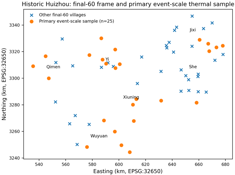
Huizhou provides a strong setting for this question. Its traditional villages combine compact lineage-based building groups, narrow alleys, courtyards, water systems and terrain-sensitive siting. Architectural studies have established inter-village organization and settlement structure [4], water landscapes and water-conservancy systems as spatial frameworks [5, 6], and regional village patterning associated with topography, water and communication [7]; however, these studies do not test whether plan-form settlement-fabric measures explain within-village thermal heterogeneity across multiple villages under a common analytical frame. At dwelling scale, tianjing and courtyard form are architecturally consequential [8, 9], while field monitoring documents the environmental role of ventilation, shading and patio conditions [10]; these site-scale findings do not establish whether the same architectural signal transfers across villages. Figure 1 locates the regional village frame used here.
Figure 1. Historic Huizhou regional analytical frame and primary village-date thermal sample. The purposive frame contains 60 villages across six county areas and predates the thermal availability and quality screening used to define the 25-village primary sample. County names in the main panel are geographic labels; Wuyuan is in present-day Jiangxi Province
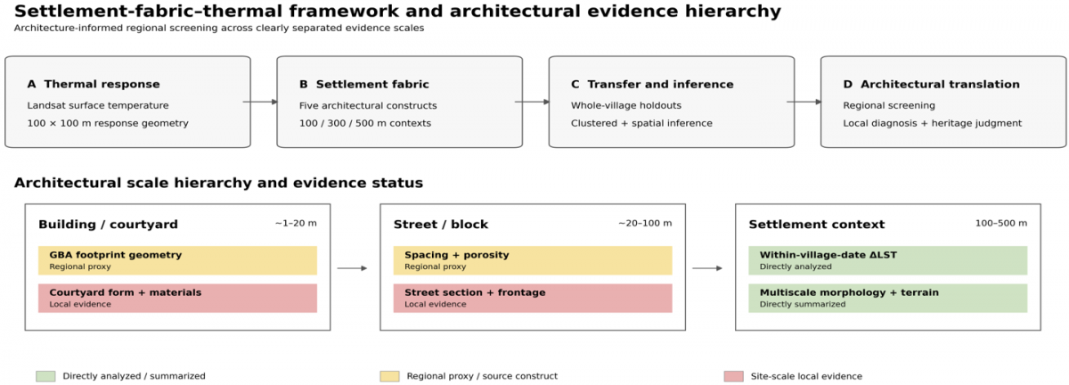
The next scale of inquiry is regional: Huizhou studies explain dwelling-, courtyard- and street-scale environmental relations, while comparable evidence is needed to test how settlement fabric relates to within-village surface-temperature heterogeneity across multiple villages. We address this scale gap through settlement fabric, the persistent plan-form, grain and configurational relations through which buildings are organized as a settlement [11-13]. Five architectural constructs represent that fabric, with terrain embedding and neighborhood-scale vertical context retained as distinct contextual layers. Figure 2 visualizes the analytical workflow and evidence hierarchy, while Table 1 translates measured metrics into architectural constructs, Huizhou spatial readings and site-scale evidence needs.
Table 1. Architectural settlement-fabric construct map. The table translates analytical metrics into architectural constructs, Huizhou spatial readings and the local evidence needed to interpret regional patterns at site scale
|
Analytical Metric(s) |
Architectural Construct |
Huizhou Spatial Reading |
Local Evidence Needed |
|
BCR |
Plan-area occupation |
Compact and continuous building-group occupation around lanes and courtyard compounds |
Courtyard geometry and material survey; vegetation/water mapping; impervious/open-surface composition |
|
Median footprint area; mean compactness |
Building-plan grain |
Mapped building-object size texture and plan compactness within the neighborhood fabric |
Building typology and floor-area information; compound identity; internal courtyard structure |
|
Clark–Evans R; nearest-neighbor spacing |
Spacing and locational regularity |
Clustering or regularity of mapped building objects within the neighborhood fabric |
Street-network topology; alley width and height-to-width ratio (H/W); connectivity; frontage continuity |
|
Aggregation; 20 m porosity |
Continuity and interstitial openness |
Continuous fabric and fine-grained gaps that may include lanes, courtyards, planted gaps or residual open space |
Courtyard/vegetation/water mapping; sky-view factor (SVF); usable open-space function |
|
Orientation coherence / entropy |
Directional order |
Local directional order potentially shaped by routes, slope and hydrological structure |
Wind-exposure assessment; facade continuity; solar-access conditions; measured street-canyon sections |
|
Slope; TPI |
Terrain embedding |
Hillside, valley and local-relief embedding of settlement fabric |
Street–slope sections; drainage mapping; measured building–water interfaces |
|
GBA median height; height IQR |
Neighborhood-scale vertical context |
Coarse neighborhood-scale variation in mapped building/roof height within the settlement fabric |
Street height-to-width ratio (H/W); sky-view factor (SVF); frontal-area density; facade continuity; field-validated storey height |
Regional comparison requires a common spatial frame while retaining architectural meaning. Landsat land-surface temperature (LST) provides spatially continuous information about surface thermal state [14], and built-environment studies show that morphology–LST relations depend on both urban form and the spatial unit used for analysis [15-17]. Recent GIS- and remote-sensing-based urban climate research has further demonstrated the value of integrating LST with spatial land characteristics to identify geographically differentiated thermal and environmental conditions [18]. Because observations within the same settlement are spatially related, whole-village holdouts provide the relevant test of generalization to unseen villages [19]. The study therefore combines a common 100 × 100 m response geometry with multiscale settlement-fabric contexts and village-held-out validation.
The architectural aim is to make regional thermal screening legible to design and conservation practice. Regional analysis identifies where relative warm/cool patterns coincide with particular settlement-fabric conditions; local architectural diagnosis then examines figure-ground, streets, courtyards, water, vegetation, materials, terrain and heritage value at the scales where those conditions can be resolved. This linkage between spatial diagnosis and conservation is consistent with landscape-based heritage approaches that treat physical form, environmental conditions, cultural significance and planning intervention as interdependent components of heritage management [20]. In this paper, a village-date event means one village observed on one qualifying Landsat acquisition date; each 100 × 100 m record nested within an event is termed an analysis-unit observation. The contribution is an architecture-informed regional screening framework that preserves a clear boundary between settlement-scale comparison and site-scale diagnosis.
Figure 2. Settlement-fabric-thermal framework and architectural evidence hierarchy. Workflow blocks A–D summarize the sequence from thermal response to settlement fabric, transfer and inference, and architectural translation. The lower panel separates building/courtyard (~1–20 m), street/block (~20–100 m) and settlement-context (100–500 m) evidence and distinguishes directly analyzed information, proxy/source constructs and site-scale local evidence. These ranges are schematic evidence bands rather than design thresholds or sensor-scale definitions. The 100 × 100 m analysis unit is the common response geometry, while 100/300/500 m define morphology contexts around that response
Accordingly, the study addresses three linked research questions.
RQ1 asks whether within-village LST patterns are repeatable across the available late-May observations in 2019 and 2024 and transferable to unseen villages and geographic domains.
RQ2 asks how much transferable information settlement-fabric morphology adds beyond terrain and which architectural constructs and tested morphology context carry the strongest transferable signal.
RQ3 asks which settlement-fabric and terrain associations remain stable under clustered and spatially robust inference and what architectural interpretation follows from those relationships.
Each georeferenced 100 × 100 m analysis unit receives a within-village-date ΔLST by comparing its Landsat-derived surface temperature with the median of the same village on the same acquisition date. Settlement fabric around the same unit is summarized at 100, 300 and 500 m using the five architectural constructs in Table 1, with terrain retained as a separate context. Whole-village holdouts then test whether these relationships generalize beyond the villages used for model fitting. The 100 m unit is the common response alignment, whereas the 300 m result is interpreted as a tested settlement context rather than a design module.
The following sections specify the regional frame, settlement-fabric measures, thermal outcome and village-held-out validation procedures used to operationalize the sequence outlined above.
2.1 Study region, village frame and village-date sample
The regional analytical frame contains 60 traditional villages across six county areas of historic Huizhou: She, Yi, Xiuning, Qimen, Jixi and Wuyuan (Figure 1). Wuyuan lies in present-day Jiangxi Province and the other five county areas in Anhui Province. The frame is treated as a purposive regional comparison frame rather than a probability sample.
The primary thermal sample was defined by Landsat availability, the quality criteria in Section 2.3, complete predictor availability and a minimum of ten valid analysis units per village-date event. It contains 1,121 analysis-unit observations nested within 33 village-date events, covering 832 unique analysis units in 25 villages.
The three qualifying acquisition dates were 24 May 2019, 28 May 2024 and 29 May 2024, contributing 663, 102 and 356 analysis-unit observations, respectively. These dates were retained because they satisfied the same Landsat availability and quality rules; their close calendar alignment within 24–29 May also provides a common late-spring seasonal frame for cross-year comparison. Two values outside the fixed 0–70 ℃ QC range were excluded before modeling. Each retained event contains at least ten analysis units satisfying both predictor and thermal criteria, and minimum valid-unit requirements from 5 to 30 units were evaluated in sensitivity analyses.
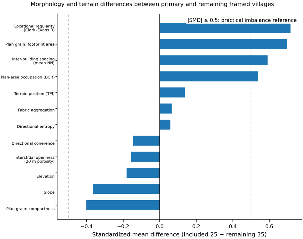
Selection balance between the 25-village thermal sample and the remaining 35 framed villages was assessed using standardized mean differences across morphology and terrain variables (Figure S1). The complementary outcome-blind weighting check used pre-outcome morphology and terrain information from the regional frame, excluding ΔLST from weight construction, and was applied only as a fixed-effect sensitivity; its directional result is reported in Section 3.6. Table 2 summarizes the study design, common response geometry, morphology contexts and analytical roles.
Table 2. Study design, data sources and analytical roles
|
Component |
Definition / Source |
Geometry / Sample / Context |
Role |
|
Study frame |
Purposive historic-Huizhou regional analytical frame |
60 villages across six county areas |
Regional frame; not a probability sample/census |
|
Primary thermal sample |
Quality-screened Landsat 8–9 village-date subset |
1,121 analysis-unit observations; 832 analysis units; 25 villages; 33 village-date events |
Primary thermal analysis sample |
|
Response geometry |
Georeferenced 100 × 100 m analysis units |
Common 100 × 100 m response alignment |
Area-weighted Landsat-derived LST estimates; common response alignment |
|
Thermal source |
Landsat 8–9 Collection 2 Level-2 Surface Temperature |
3 qualifying acquisition dates |
QA_PIXEL bits 0–5 clear; ST_QA ≤ 2 K; cloud distance ≥ 1 km; valid area ≥ 50% |
|
Built morphology |
GlobalBuildingAtlas static morphology representation |
100, 300 and 500 m morphology contexts |
Settlement-fabric morphology metrics; 300 m primary morphology context |
|
Terrain |
FABDEM |
Elevation, slope and TPI |
Terrain controls and alternative explanation |
|
Primary outcome |
Within-village-date LST anomaly |
LST − village×date median LST |
Relative within-village surface-temperature anomaly; distinct from air temperature and long-term heat-buffering capacity |
|
Weighting |
Event-equal weights |
1/n analysis units per village-date event |
Prevents large events dominating loss/inference |
2.2 Architectural settlement-fabric representation and terrain embedding
The settlement-fabric representation uses four linked levels: metrics are computed variables, constructs group those variables architecturally, the Huizhou spatial reading interprets the constructs at regional scale, and local evidence identifies what is needed for site-scale diagnosis. Five architectural construct groups were used: plan-area occupation, building-plan grain, spacing and locational regularity, continuity and interstitial openness, and directional order. Building metrics were derived from GlobalBuildingAtlas (GBA), an open product of building polygons and heights [21]. Plan-area occupation is quantified by building coverage ratio (BCR), while Clark–Evans R follows the nearest-neighbor regularity formulation of Clark and Evans [22]; the remaining metrics describe object grain, spacing, aggregation/open gaps and orientation.
GBA is based mainly on 2019 PlanetScope imagery, with 2018 imagery used where necessary, so the morphology layer is treated as a static circa-2018/2019 representation for both thermal years. Slope and topographic position index (TPI) from FABDEM [23] describe terrain embedding.
GBA median height, height interquartile range, height coefficient of variation and a simple volume-density proxy provide neighborhood-scale vertical context. They were tested separately from the primary 2D morphology set so that vertical context could be evaluated without changing the primary comparison among terrain, settlement morphology and their combination. Table 1 shows the principal vertical-context descriptors used for architectural reading; the complete GBA-derived vertical-context sensitivity, based on the 3D building-height product, is reported in Table S1.
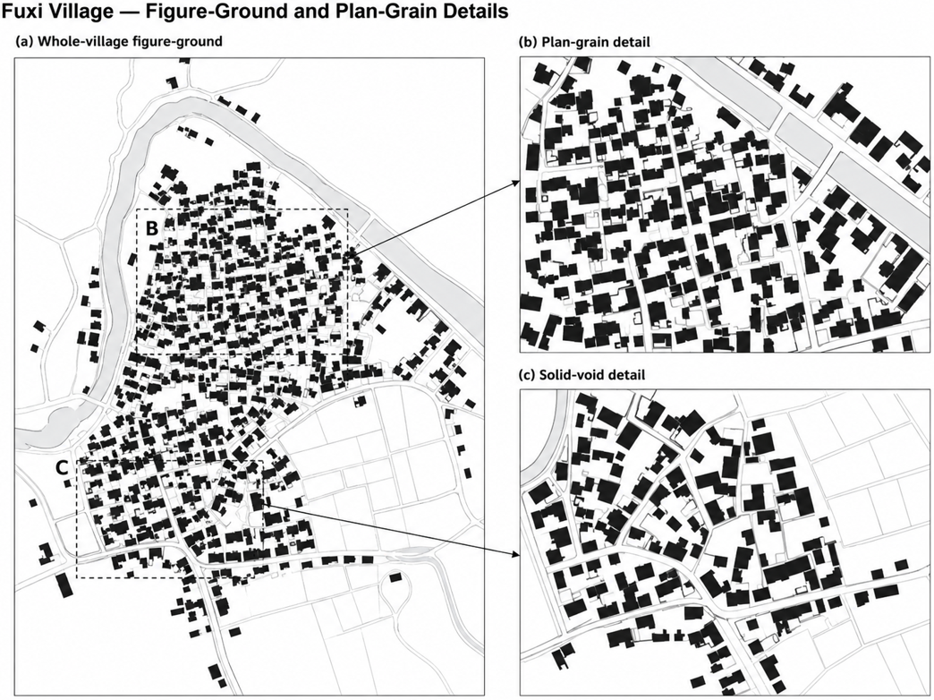
Figure 3 provides an illustrative architectural plan-reading reference for interpreting the settlement-fabric constructs in Table 1 at plan scale. Fuxi Village is included in the thermal sample, and the figure-ground reading is derived from the same regional building/morphology database used to construct the settlement-fabric predictors.
Figure 3. Fuxi Village figure-ground and plan-grain reading derived from the regional building/morphology database. Panel (a) shows the whole-village solid–void pattern; dashed detail windows B and C correspond to panels (b) and (c), which highlight plan-grain and solid–void relations
Table 1 maps these metrics to their architectural reading and evidence boundary. The construct framework follows established urban-morphology concepts of tissue, grain, plan form and morphological structure [11-13].
Within this framework, high plan-area occupation (BCR) can coexist with narrow lanes and internal tianjing voids; open gaps between building masses may contain lanes, courtyards, planting, water edges or residual space; and directional order may reflect routes, slope or hydrological structure. The regional measures therefore identify spatial conditions for closer architectural diagnosis while local evidence resolves their detailed spatial meaning.
Across whole-village and detail views, the Fuxi figure-ground plate links solid–void pattern, plan grain, adjacency and interstitial space to the regional construct vocabulary.
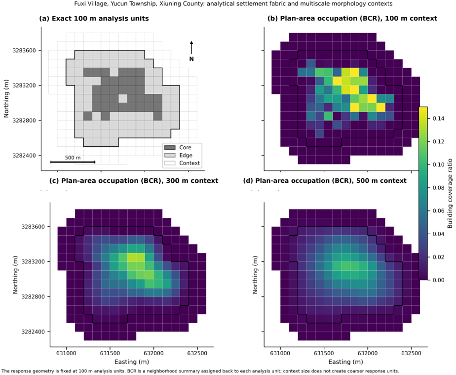
The georeferenced 100 × 100 m analysis unit was retained as the common response geometry. Settlement morphology was summarized around the same unit at 100, 300 and 500 m; these distances define the surrounding morphology context and do not create new thermal pixels. The 300 m context was used for the primary models, while 100 and 500 m were retained for the common-sample scale comparison. Figure 4 uses Fuxi Village, Yucun Township, Xiuning County, to show the same analysis units embedded in the three morphology contexts.
Fuxi Village was selected because it provides two-date 2019/2024 coverage and broad analysis-unit coverage, allowing the multiscale geometry to be shown clearly. Figure 4 illustrates how the same response geometry can be read within progressively broader settlement contexts without changing the response unit itself.
Figure 4. Fuxi Village, Yucun Township, Xiuning County: analysis units and multiscale morphology context. Panel (a) shows the 100 × 100 m core, edge and context analysis units; panels (b–d) map GBA-derived building coverage ratio (BCR) summarized at 100, 300 and 500 m and assigned to the same analysis units. The context radius denotes the neighborhood used to summarize settlement fabric and does not create a coarser thermal response unit. These panels present the analytical morphology representation used for regional comparison
Core/edge/context labels describe each analysis unit relative to the GBA-derived settlement extent; they are spatial descriptors rather than cadastral, administrative or statutory heritage boundaries.
The modeled regional covariates comprise settlement morphology, terrain and the tested neighborhood-scale vertical context; independent vegetation, water and impervious/open-surface fractions remain part of the finer local evidence layer.
2.3 Landsat-derived surface temperature and quality control
Thermal estimates came from Landsat 8–9 Collection 2 Level-2 Surface Temperature (ST) products [24, 25]. The distributed product is provided on a 30 m grid, while the TIRS thermal bands have approximately 100 m native sampling. The 100 × 100 m analysis units are therefore georeferenced aggregation polygons over the ST product rather than independent sensor pixels. The operational LST retrieval is described by Malakar et al. [26] within the broader Landsat 8 science framework [27].
Source-pixel ST values were intersected exactly with each analysis unit and area-weighted. Valid observations required clear QA_PIXEL bits 0–5, ST_QA ≤ 2.0 K, cloud distance ≥ 1 km and at least 50% valid area. Scaled ST integers were converted using ST(K) = DN × 0.00341802 + 149.0 and then to ℃ following USGS guidance [25]. Each retained thermal estimate was linked to the same georeferenced analysis-unit geometry used throughout the study.
Because the analysis units are aggregation geometry over the thermal product, grouped validation, Moran/Conley diagnostics and a separate response-aggregation test address spatial dependence and scale sensitivity. Quality sensitivities applied a 75% valid-area rule, a 2 km cloud-distance rule and minimum valid-unit requirements of 5, 10, 15, 20 and 30 units per village-date event; the corresponding results are reported in Table 3.
Table 3. Thermal-quality and minimum-valid-unit sensitivity analyses, including the 2 km cloud-distance check
|
Sensitivity |
Rule |
Rows |
Villages |
Events |
Ridge R² |
|
Primary valid-unit requirement |
village-date n ≥ 10 |
1,121 |
25 |
33 |
0.381 |
|
Stricter valid fraction |
valid fraction ≥ 0.75 |
964 |
21 |
27 |
0.479 |
|
Stricter cloud distance |
cloud distance ≥ 2 km |
1,121 |
25 |
33 |
0.381 |
|
Minimum valid units ≥ 5 |
village-date n ≥ 5 |
1,134 |
27 |
35 |
0.388 |
|
Minimum valid units ≥ 15 |
village-date n ≥ 15 |
1,023 |
19 |
25 |
0.508 |
|
Minimum valid units ≥ 20 |
village-date n ≥ 20 |
921 |
15 |
19 |
0.557 |
|
Minimum valid units ≥ 30 |
village-date n ≥ 30 |
748 |
9 |
12 |
0.549 |
2.4 Within-village-date thermal outcome and event-equal weighting
For analysis unit i in village v on date t, the outcome was defined as:
ΔLST(i,v,t) = LST(i,v,t) − median[LST(v,t)]
Centering within each village-date event converts the response into a relative thermal pattern: positive values identify locations warmer than the contemporaneous village median and negative values identify cooler locations. The comparison therefore focuses on spatial differences inside the same village under the same Landsat overpass rather than on absolute temperature differences between villages or years.
Because events contained different numbers of valid units, each observation received weight 1/n(v,t), giving every village-date event equal total weight in model fitting and primary performance metrics.
2.5 Predictive models and grouped validation
This stage tests whether settlement-fabric relationships generalize to villages not used for model fitting. Ridge regression was the primary transfer model because it handles correlated predictors while retaining a transparent linear structure [28]. Predictors were standardized within each training fold; α = 1.0 was used for the primary model, with α = 0.1 and 10 as sensitivity checks. Random Forest regression [29] provided a nonlinear comparison, with implementation settings reported in the APPENDIX.
Primary transfer performance used five-fold village-grouped cross-validation (implemented with GroupKFold), holding out whole villages so that all analysis units from a village remained in the same fold. R², RMSE and MAE were calculated with event-equal weights. Alternative tests used geographic village folds, leave-three-county combinations, joint date-and-county holdouts and leave-one-Landsat-scene-out validation; an unweighted repetition tested the nested-model ordering [19, 20]. Local-coordinate controls used the planar centroid coordinates of the georeferenced analysis units as simple positional covariates; they were evaluated with terrain and with the full morphology + terrain transfer set under the same village folds to test whether the fabric constructs retained predictive value beyond simple spatial position; the comparison is reported with the predictor-set results in Section 3.4.
2.6 Panel inference, multiplicity and spatial dependence
This stage asks which associations remain stable after accounting for clustered and spatially correlated uncertainty. Predictive transfer and predictor-level inference use related but distinct variable sets. The transfer benchmark uses nine morphology predictors—plan-area occupation (BCR), median footprint area, mean compactness, mean nearest-neighbor distance, Clark–Evans R, aggregation index, 20 m porosity, orientation coherence and orientation entropy—plus elevation, slope and TPI, giving 12 predictors for morphology + terrain. The inferential specification uses 11 predictors. Outcome-blind prefit collinearity screening used variance inflation factors (VIFs); after mean nearest-neighbor distance was omitted, the retained 11-predictor set remained below the pre-specified VIF threshold. The remaining eight morphology predictors plus elevation, slope and TPI are reported in Tables S2a–b.
Model specification. Event-equal weighted least squares used the 11-predictor inferential set with village and acquisition-date fixed effects. Because morphology and terrain predictors are time-invariant at unit level, inference uses village and acquisition-date fixed effects rather than analysis-unit fixed effects. Village×date fixed effects and a centered plan-area occupation (BCR) × median-height interaction provided additional checks on event alignment and neighborhood-scale vertical context.
Uncertainty and robustness. Uncertainty was evaluated with village-clustered standard errors, Benjamini–Hochberg false-discovery-rate control [30], 50,000-draw village-level wild-cluster tests (a finite-sample cluster-robust check) and Conley spatial-HAC covariance (a distance-based covariance correction). Residual spatial dependence was evaluated with Moran’s I [31]. Conley spatial-HAC covariance [32] used analysis-unit centroid distances in EPSG:32650 with a Bartlett kernel at 200 m, 500 m and 1 km within village-date events; a same-date sensitivity extended the distance range to 1, 5 and 10 km across villages. These alternatives change the uncertainty model while leaving fitted coefficient estimates unchanged; complete predictor-level results are reported in Tables S2a–b.
2.7 Scale and complementary robustness analyses
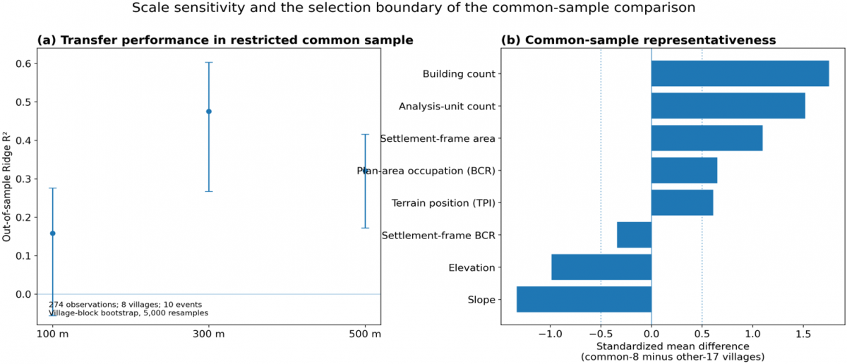
Scale comparison. To test whether the regional relationship depends on morphology context, transfer was compared at 100, 300 and 500 m using analysis-unit observations complete at all three contexts. Re-applying the minimum 10-valid-unit requirement produced a common sample of 274 observations from eight villages and ten village-date events. The same village-grouped model was used at all three contexts, with village-block bootstrap uncertainty and a representativeness comparison against the other primary villages (Figure S2; Tables S3a–b).
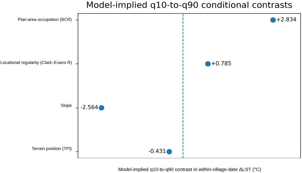
Complementary morphology checks. Model-implied q10-to-q90 conditional contrasts summarize the difference in ΔLST between low (10th-percentile) and high (90th-percentile) predictor values while the fitted model holds other terms fixed; coefficient uncertainty is evaluated with Conley and wild-cluster procedures. Linear and spline plan-area occupation (BCR) responses were compared to evaluate response form and the presence of a strong threshold.
Additional robustness checks. Complementary checks evaluate selection weighting (Section 3.6), GBA-derived vertical-context sensitivity (Table S1), minimum valid-unit and thermal-quality sensitivity (Table 3), and response aggregation (Table S4). Section 3.6 examines plan-area occupation (BCR) response form and neighborhood-scale vertical context alongside the primary inferential analysis.
A separate response-aggregation test combined the quality-screened 100 m summaries into georeferenced 200 m blocks. LST was re-aggregated with the original valid-area weights and re-centered by village-date; morphology and terrain predictors were averaged across contributing 100 m analysis units. The test retained the original village folds and event-equal weighting and compared blocks with at least two, at least three, and all four contributing 100 m analysis units (Table S4). This isolates a change in response aggregation from the 100/300/500 m morphology-context comparison, which keeps the 100 m response geometry fixed.
Analytical scope. The study focuses on relative surface-temperature heterogeneity within the three qualifying late-May acquisitions in 2019 and 2024. Model output is interpreted as regional settlement-fabric screening that identifies locations and fabric conditions for finer architectural diagnosis.
Results follow the research questions: RQ1 combines repeatability and cross-village transfer (Sections 3.2–3.3), RQ2 combines construct hierarchy and morphology context (Sections 3.4–3.5), and RQ3 examines predictor-level robust associations (Section 3.6).
3.1 Sample characteristics and spatial pattern overview
The retained sample provides analysis-unit observations nested within village-date events across the three qualifying late-May acquisitions in 2019 and 2024 (Table 2, Figure 1). Event-equal weighting gives each village-date event equal total influence despite differences in the number of valid analysis units.
Across the three acquisitions, median within-village-date ΔLST is zero by construction, while its spatial dispersion differs among village-date events. This repeated-unit structure enables comparison of relative surface-temperature anomalies within villages rather than village mean temperatures.
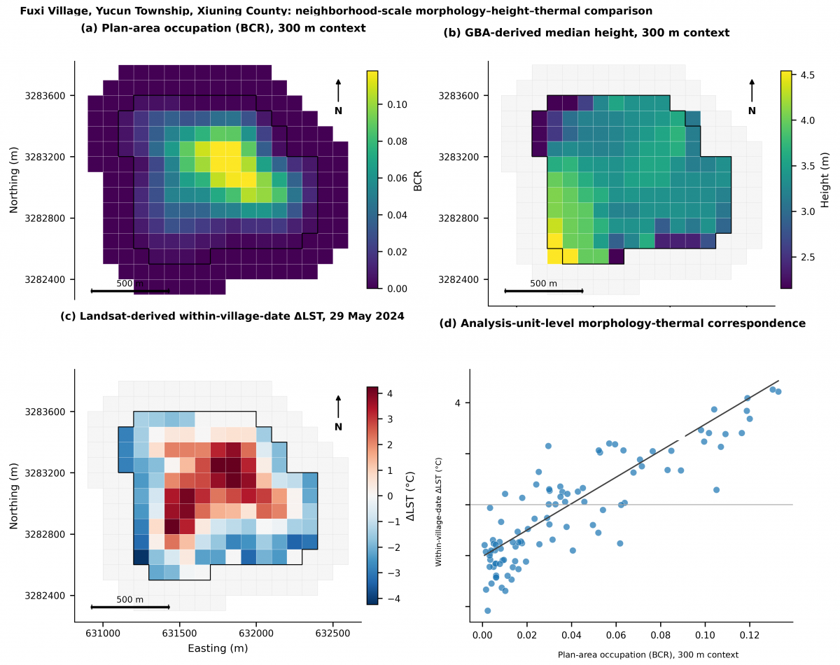
Figures 4 and 5 show the shared analysis geometry for Fuxi Village. Figure 4 demonstrates the 100 m response units and 100/300/500 m morphology contexts; Figure 5 places 300 m plan-area occupation (BCR), GBA median height and the 29 May 2024 within-village-date ΔLST on that common frame. The retained 25 villages show moderate morphology and terrain differences from the other 35 framed villages, with the largest contrasts in spacing/regularity, plan grain and plan-area occupation (Figure S1).
Figure 5. Fuxi Village, Yucun Township, Xiuning County: neighborhood-scale morphology–height–thermal comparison. Panels show (a) 300 m-context plan-area occupation, quantified by building coverage ratio (BCR), assigned to 100 × 100 m analysis units, (b) GBA-derived median building height at the same 300 m morphology context, (c) Landsat-derived within-village-date ΔLST on 29 May 2024, and (d) the analysis-unit-level plan-area occupation (BCR)–ΔLST scatter. Height is shown as a static GBA neighborhood-scale context proxy; the plan-area occupation (BCR) × height interaction is evaluated separately in Section 3.6
3.2 Cross-year repeatability of within-village thermal patterns
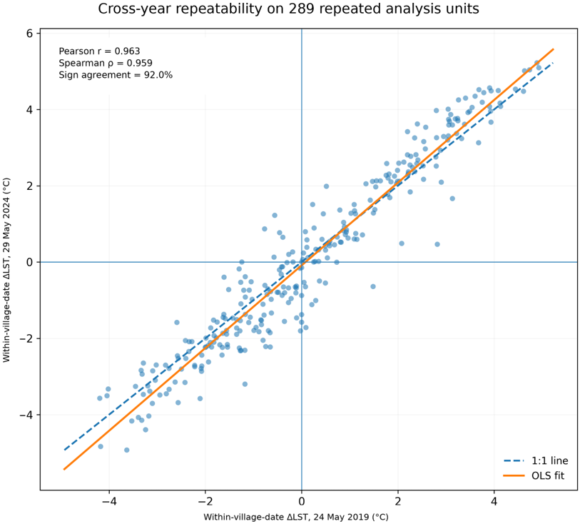
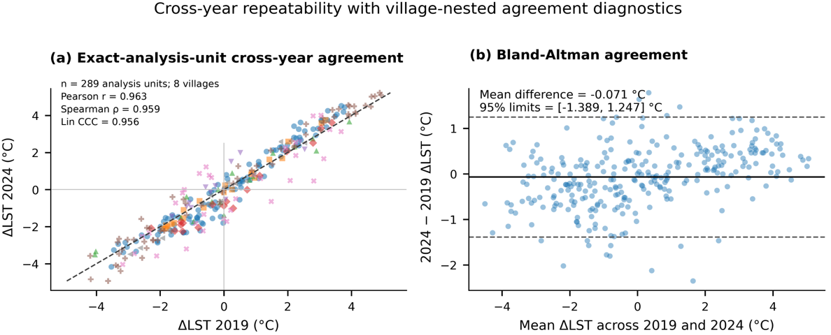
The direct cross-year test matched 289 identical 100 × 100 m analysis units observed on 24 May 2019 and 29 May 2024 in eight villages. Pearson r was 0.963, Spearman ρ was 0.959, 92.0% of units retained the same warmer/cooler sign, and the between-year anomaly RMSE was 0.675 ℃ (Figure 6).
Figure 6. Cross-year repeatability for the same 289 georeferenced analysis units observed on 24 May 2019 and 29 May 2024. Pearson and Spearman agreement and sign consistency are descriptive at analysis-unit level; uncertainty is evaluated with village-block procedures in Supplementary Figure S3 and Tables S5a–b
Matching identical georeferenced positions isolates repeatability of the warm–cool ordering across years, while village-block procedures account for nesting within the eight settlements represented in both acquisitions.
Village-block resampling and leave-one-village-out checks confirmed that the matched-position agreement remains strong when village nesting is respected (Supplementary Figure S3, Tables S5a–b).
The matched positions therefore show a stable late-May warm–cool ordering across the two observed years.
3.3 Cross-village and geographic transferability
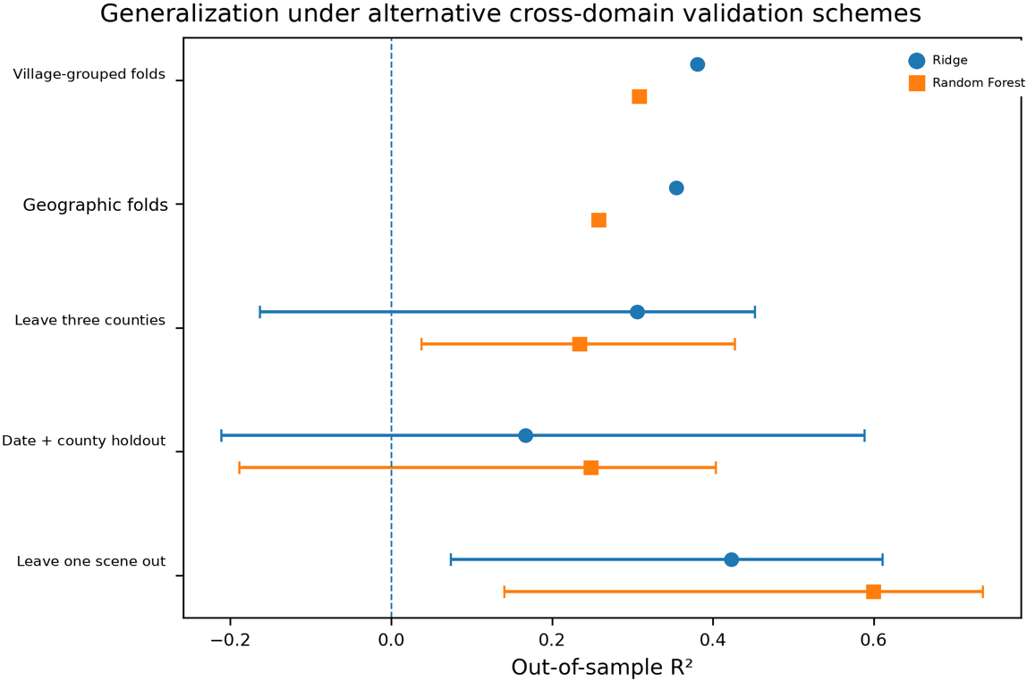
Generalization to unseen villages was evaluated with the 12-predictor morphology + terrain transfer set (nine morphology predictors plus elevation, slope and TPI) under alternative validation schemes with stronger domain separation, using Ridge as the primary transparent model and Random Forest as a nonlinear comparison (Table 4).
Table 4. Transfer performance under alternative cross-domain validation schemes using the 12-predictor morphology + terrain transfer set (nine morphology predictors plus elevation, slope and TPI)
|
Model |
Validation |
R² |
RMSE (℃) |
Robustness Note |
|
Ridge |
Village-grouped cross-validation |
0.381 |
1.543 |
Five village-held-out folds |
|
Ridge |
Geographic village folds |
0.355 |
1.575 |
Geographic blocking |
|
Ridge |
Leave three counties out |
0.306 |
1.614 |
Positive 18/20; min −0.163 |
|
Ridge |
Joint date + county holdout |
0.167 |
1.801 |
Positive 8/9; min −0.211 |
|
Ridge |
Leave one Landsat scene out |
0.423 |
1.527 |
Positive 5/5; min 0.074 |
|
Random Forest |
Village-grouped cross-validation |
0.308 |
1.631 |
Five village-held-out folds |
|
Random Forest |
Geographic village folds |
0.258 |
1.689 |
Geographic blocking |
|
Random Forest |
Leave three counties out |
0.234 |
1.678 |
Positive 20/20; min 0.038 |
|
Random Forest |
Joint date + county holdout |
0.248 |
1.730 |
Positive 8/9; min −0.189 |
|
Random Forest |
Leave one Landsat scene out |
0.599 |
1.184 |
Positive 5/5; min 0.141 |
All nested predictor-set comparisons used the same five village folds, and the terrain-only < morphology-only < morphology + terrain ordering persisted under unweighted fitting and alternative Ridge penalties.
Overall performance remained positive under each validation scheme, while a small number of constituent holdouts fell below zero under the strongest county/date separation. These cases identify settings where local calibration or additional environmental evidence can refine the regional reading (Figure 7, Table 4).
Figure 7. Generalization under alternative cross-domain validation schemes using the 12-predictor morphology + terrain transfer set. Ridge is the primary transparent model and Random Forest provides nonlinear comparison. Points show the overall out-of-sample R² for village-grouped folds, geographic folds, joint date+county holdout and leave-one-scene-out validation; for the 20 leave-three-county combinations, the point is the median R². Where a scheme contains multiple explicit holdouts, horizontal bars span the observed minimum-to-maximum R² across constituent holdouts
Together with the matched-position repeatability result, the holdouts show that the regional cross-village settlement-fabric transfer signal remains useful beyond the villages used for model fitting.
3.4 Architectural hierarchy of settlement-fabric associations
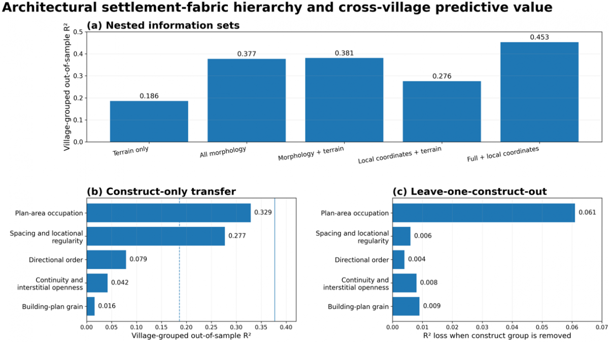
The construct-level analysis provides the clearest architectural result. Plan-area occupation (BCR) showed the strongest standalone cross-village transfer (R² = 0.329), followed by spacing and locational regularity (R² = 0.277). Removing plan-area occupation produced the largest loss from the full morphology model (ΔR² = 0.061), while directional order, continuity and interstitial openness, and building-plan grain showed lower standalone regional predictive value (Figure 8, Table S6).
Together, these results place figure-ground occupation and inter-building configuration at the center of the regional settlement-fabric signal. Plan-area occupation expresses how strongly building mass occupies the neighborhood plan, while spacing and locational regularity describe the arrangement of mapped building objects. This construct-group ranking is distinct from predictor-level inferential support: the spacing/regularity construct contains both mean nearest-neighbor distance and Clark–Evans R, whereas Clark–Evans R is the individual spacing variable carried forward in the robust coefficient interpretation. Building-plan grain, continuity and interstitial openness, and directional order provide complementary contextual description around those stronger regional signals.
At predictor-set level, morphology transferred substantially better than terrain alone, while adding terrain to the morphology set changed performance only modestly. This indicates that settlement fabric carries cross-village spatial information beyond elevation, slope and terrain position (Figure 8).
Two complementary checks reinforce the same reading: GBA-derived vertical-context terms add little beyond the primary 2D morphology set at this scale (the GBA-derived vertical-context sensitivity is reported in Table S1), and local-coordinate controls in Figure 8 show additional spatial structure without removing the settlement-fabric contribution.
The hierarchy identifies which architectural constructs carry the regional signal; the following context analysis asks at which tested morphology context that signal is strongest.
Figure 8. Predictor-set transfer and architectural construct hierarchy under identical event-equal five-fold village-grouped validation. Panel (a) reports predictor-set transfer, comparing terrain-only, morphology-only and morphology + terrain models together with local-coordinate controls; the figure label “full + local coordinates” denotes the 12-predictor morphology + terrain transfer set plus centroid coordinates. Panels (b–c) report construct-level hierarchy and sensitivity: panel (b) shows construct-only cross-village R² and panel (c) the R² loss when each construct group is removed from the nine-predictor morphology set. Predictor-level coefficient stability is evaluated separately in Section 3.6. The local-coordinate models test whether measured fabric constructs add predictive value beyond simple spatial position and terrain
3.5 Morphology-context and response-aggregation sensitivity
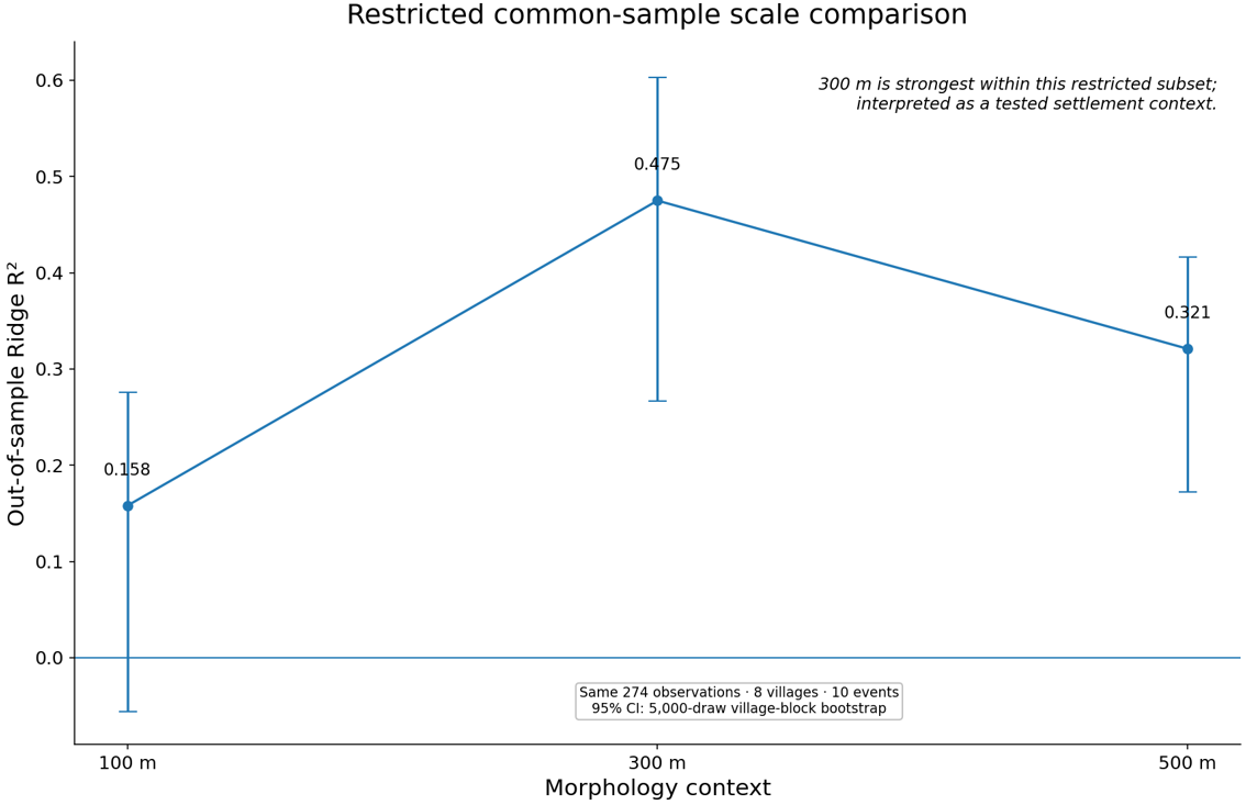
In the restricted common-sample comparison, 300 m gives the strongest transfer among the three tested morphology contexts, with village-block uncertainty remaining above zero for that context (Figure 9, Figure S2, Table S3a). The common-sample villages are generally larger, flatter and lower than the other primary villages (Table S3b), so the result is read as a context finding for this subset rather than as a universal optimum.
Figure 9. Restricted common-sample scale comparison with village-block uncertainty. The same 274 observations, eight villages and ten village-date events are evaluated at 100, 300 and 500 m morphology contexts. Points show out-of-sample Ridge R² and error bars show 95% confidence intervals from 5,000 village-block bootstrap resamples. The 300 m result is interpreted as a subset-specific settlement-context finding rather than a universal design radius
The separate 200 m response-aggregation test is sensitive to how many contributing 100 m analysis units are required (Table S4). Morphology-only and morphology + terrain transfer remain positive under the ≥2-contributor definition, then cross below zero under the stricter ≥3 and complete four-unit definitions as the sample contracts. The two scale tests address different questions: 300 m changes the context from which morphology is summarized, whereas 200 m aggregation changes the thermal response aggregation and sample composition.
The 300 m context therefore carries the strongest tested morphology signal in this restricted sample, while response aggregation remains a separate analytical choice.
3.6 Predictor-level settlement-fabric and terrain associations
Conditional association magnitude. Model-implied contrasts show warmer relative surface-temperature anomalies with increasing plan-area occupation and locational regularity, and cooler relative anomalies with increasing slope and terrain position. Plan-area occupation has the largest morphology contrast, while Table 5 provides the corresponding coefficient magnitudes and uncertainty. Figure 10 summarizes these q10-to-q90 conditional contrasts for the four consistently supported variables.
Table 5. Consistently supported settlement-fabric and terrain associations under 1 km Conley spatial-HAC inference and complementary wild-cluster tests
|
Term |
Panel Coef |
Conley SE |
Conley 95% CI |
Conley p |
Wild-Cluster p |
Conditional Contrast (℃) |
|
Plan-area occupation (BCR, 300 m) |
11.745 |
0.894 |
[9.993, 13.497] |
<0.001 |
<0.001 |
2.834 |
|
Locational regularity (Clark–Evans R, 300 m) |
1.055 |
0.283 |
[0.500, 1.610] |
<0.001 |
0.028 |
0.785 |
|
Slope |
-0.141 |
0.010 |
[-0.161, -0.120] |
<0.001 |
<0.001 |
-2.564 |
|
Terrain position (TPI, 300 m) |
-0.041 |
0.011 |
[-0.062, -0.019] |
<0.001 |
0.011 |
-0.431 |
Figure 10. Model-implied q10-to-q90 contrasts for the four consistently supported variables. Points show descriptive conditional contrasts; coefficient-level uncertainty is reported in Table 5 using Conley and wild-cluster procedures. These contrasts are interpreted as conditional within-village-date associations, while site-specific effects are evaluated through separate local evidence
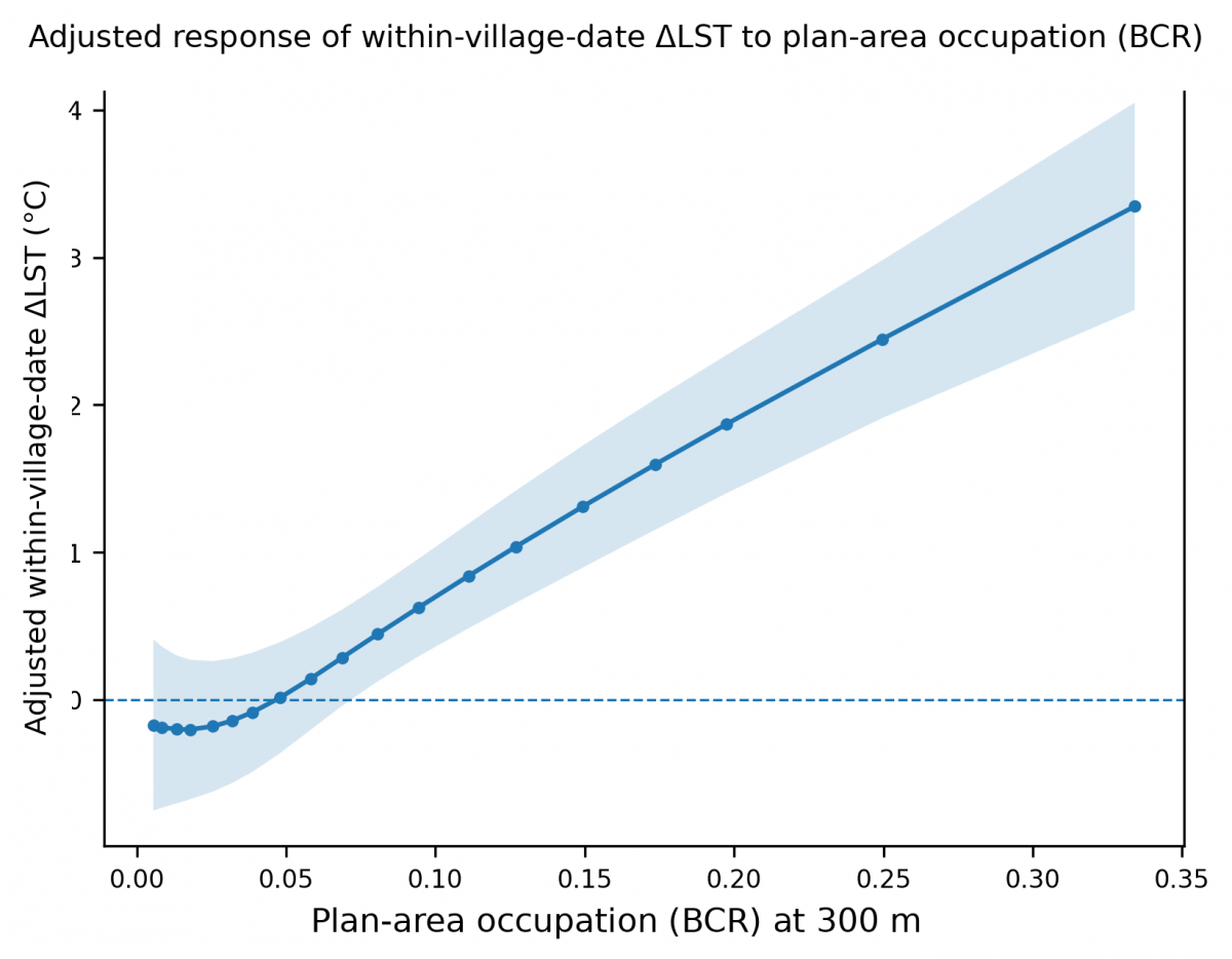
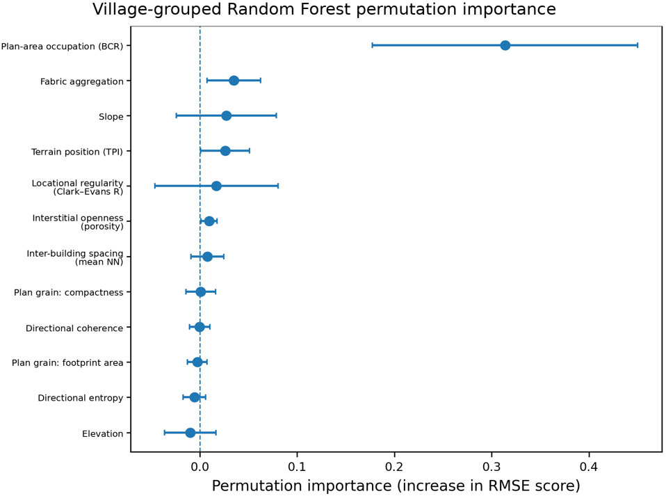
The adjusted plan-area occupation (BCR) response is predominantly monotonic over the observed range, with little evidence that added spline flexibility improves the interpretation (Figure 11). Random Forest permutation importance also places plan-area occupation (BCR) first in the nonlinear comparison (Supplementary Figure S4).
Figure 11. Adjusted response of within-village-date ΔLST to plan-area occupation (BCR) at 300 m. The response is predominantly monotonic and indicates a gradual relation rather than a sharp universal threshold
The plan-area occupation (BCR) × height diagnostic gives the same architectural reading: the plan-area occupation association remains clear, while median height and the interaction add little at this neighborhood-scale context. Height therefore remains a simple contextual descriptor rather than a substitute for site-scale vertical geometry.
Robust inference. Across clustered/FDR, wild-cluster and Conley procedures, the same four variables are consistently supported: plan-area occupation (BCR) and locational regularity (Clark–Evans R) are positive, while slope and terrain position (TPI) are negative. Table 5 reports coefficient magnitudes and uncertainty, and Tables S2a–b provide the complete 11-predictor results.
The remaining predictors show more method-dependent support across the complementary procedures. This keeps the regional inferential emphasis on the four consistently supported variables rather than extending the architectural interpretation to every measured metric.
The same four directions persist under broader same-date spatial covariance and village × date fixed effects. Residual Moran’s I indicates spatial structure in the settlement signal, while the complementary uncertainty treatments preserve the same architectural reading.
The outcome-blind selection-weighted fixed-effect check preserved the positive plan-area occupation (BCR) and Clark–Evans R directions and the negative slope and TPI directions, providing a complementary sample-selection sensitivity. The corresponding directional check is documented in the APPENDIX under “Selection-weighted outcome sensitivity.”
Minimum valid-unit and thermal-quality sensitivities likewise preserve positive Ridge transfer across the tested rules (Table 3). The 2 km cloud-distance rule reproduced the primary 1,121-observation sample and Ridge performance (R² = 0.381). Stricter minimum valid-unit requirements increase within-event coherence while narrowing geographic coverage, framing that sensitivity as a coverage–coherence trade-off.
These associations provide the empirical basis for the architectural interpretation developed in Section 4.4.
The discussion follows the architectural evidence sequence: repeatability and transfer establish the value of regional comparison, construct and scale results show how settlement fabric can be read regionally, and robust associations are translated into local architectural diagnosis.
4.1 Repeatability and transfer establish a regional screening signal
For RQ1, cross-year repeatability and cross-village generalization provide complementary evidence for regional comparison. Matched late-May locations preserve their warm–cool ordering across 2019 and 2024, and overall out-of-sample performance remains positive under each validation scheme. Most constituent holdouts are positive; the few below-zero cases occur under the strongest county/date separation and identify where additional local calibration can refine the regional reading.
The value lies in the comparison itself. Centering temperature within each village focuses attention on spatial differences inside a settlement, and holding out entire villages asks whether settlement-fabric relationships learned elsewhere retain out-of-sample value in a new one. This pairing separates within-village thermal patterning from cross-village generalization.
4.2 Plan-area occupation leads the settlement-fabric hierarchy
For the construct component of RQ2, the hierarchy is architecturally more informative than a flat predictor list. Plan-area occupation leads the regional transfer hierarchy, while the spacing and locational regularity construct provides the second strongest construct-level signal. These two constructs distinguish occupation from configuration: one reads how strongly building mass occupies the plan, the other how mapped building objects are arranged. Similar occupation levels can contain different lane, tianjing, planted or water-linked gaps and surface conditions, so plan-area occupation (BCR) is read as a screening descriptor rather than a direct design prescription.
Site-scale evidence for lane and courtyard geometry, vegetation, water edges, materials and heritage fabric resolves the local spatial meaning of the regional descriptors [5, 6]. Building-plan grain, continuity/interstitial openness and directional order remain complementary descriptors for that local plan reading.
Regional surface temperature and pedestrian microclimate operate at different scales. Huizhou and related traditional-settlement research resolves height-to-width ratio (H/W), orientation, interface opening, water/green ratios and tianjing form [33-37]. GBA median height and height variability provide only neighborhood-scale vertical context; detailed street-canyon geometry, sky-view factor (SVF) and frontage continuity belong to the site-scale architectural diagnostic layer.
4.3 The 300 m result is a settlement context, not a design radius
For the scale component of RQ2, the analysis is best read as a settlement-context result. In the restricted common sample, 300 m provides the strongest performance among the tested morphology contexts. Architecturally, that context can span several adjoining building groups, lanes and open-space sequences, allowing occupation, spacing and directional order to be read as a local piece of settlement fabric around the 100 m response geometry. Figure 4 makes the distinction visible: the morphology context changes, while the response geometry remains the same. The 300 m result therefore describes settlement context rather than a courtyard module, street-section threshold or conservation radius.
The complementary 200 m aggregation sensitivity reinforces the same distinction: morphology-based transfer crosses below zero under the stricter ≥3 and complete four-unit definitions as sample coverage contracts. Context scale and response aggregation therefore answer different questions—the 300 m result concerns the neighborhood from which morphology is summarized, whereas the 100 m analysis unit is the common response alignment used in the primary analysis.
4.4 Robust associations sharpen the architectural reading
For RQ3, the stable predictor-level directions sharpen the architectural reading. Plan-area occupation (BCR) and locational regularity (Clark–Evans R) provide the consistently stable morphology directions, while slope and terrain position form the terrain-embedding context. Read together, they frame regional surface-temperature heterogeneity as a joint fabric–terrain condition rather than a single plan-occupation measure.
Architecturally, slope and TPI locate settlement fabric within hillside, valley and local-relief settings, broadening screening from plan occupation/configuration to terrain embedding. These regional associations are best carried forward as terrain-embedding cues; site-scale street–slope sections, drainage relationships and measured building–water interfaces provide the evidence needed for mechanism-specific interpretation.
4.5 Architecture-informed screening and heritage-compatible local diagnosis
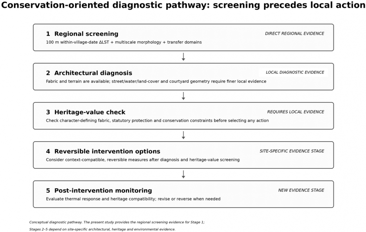
The architecture and conservation translation is organized as a proposed five-stage diagnostic pathway (Figure 12). Regional screening identifies Landsat-derived surface-temperature patterns, while site-scale evidence is required to evaluate pedestrian microclimate and design performance. Georeferenced 100 × 100 m analysis units remain embedded in explicit multiscale settlement contexts, and the construct vocabulary established in Table 1 keeps the regional model legible in architectural terms.
The Fuxi Village figure-ground reference (Figure 3) and the Fuxi analytical views (Figures 4–5) bridge regional metrics and plan reading: the former shows solid–void grain and adjacency, while the latter locates the response geometry and morphology contexts used in the regional analysis.
Figure 12. Conservation-oriented five-stage diagnostic pathway. Regional analysis provides the screening layer; site-scale architectural evidence provides the local diagnostic layer. Heritage-value review precedes consideration of reversible intervention options, and post-intervention monitoring forms a distinct evidence stage. The pathway is conceptual, with site-specific evidence guiding any local intervention assessment
Within this pathway, Stage 1 uses regional screening to identify relative warm/cool areas together with their settlement-fabric context. Stage 2 adds local figure-ground, street, courtyard/open-space, water, vegetation, material, terrain and vertical-enclosure evidence. Stage 3 evaluates heritage value and character-defining fabric. Stage 4 considers reversible or low-impact options grounded in that diagnosis, and Stage 5 monitors both thermal and conservation outcomes. This sequence follows conservation principles of significance, authenticity, cautious change and minimum necessary intervention and keeps architectural and conservation judgment between regional screening and any site-specific action. Table 6 summarizes these evidence needs; the checklist organizes evidence requirements for site-specific assessment, with local heritage and performance review governing any intervention decision. Stages 3–5 function as conceptual decision stages; their use depends on site-specific heritage and performance evidence rather than intervention-effect estimates from the regional analysis.
Table 6 groups six local conditions with the corresponding architectural, environmental and heritage evidence. The regional BCR association helps prioritize inspection, while site-scale evidence determines how those conditions are interpreted in conservation practice.
Table 6. Diagnostic evidence checklist for conservation screening and local architectural assessment. The entries define evidence needs for site-specific assessment; heritage significance and locally established environmental effects guide any subsequent action. The review-intensity terms are indicative categories within this conceptual workflow, not statutory approval classifications
|
Local Diagnostic Consideration |
Heritage Review Priority |
Evidence Needed for Site-Specific Assessment |
Interpretive Status |
|
Existing vegetation and water-edge condition |
Routine local heritage review |
Local vegetation/water diagnosis; confirm continuity of character-defining fabric |
Existing condition for conservation-compatible local assessment; thermal effect to be established locally |
|
Potential reversible/seasonal shading condition in non-character-defining spaces |
Focused local heritage review |
Street/courtyard microclimate + heritage-value check |
Candidate for site-specific testing |
|
Non-character-defining hard-surface and permeability condition |
Focused material and drainage review |
Material, drainage, water-edge and heritage review |
Candidate for site-specific testing; BCR is a screening relation |
|
Historic alley-section and frontage condition |
Detailed conservation review |
Site-scale architectural conservation assessment of historic alley section and frontage |
Requires architectural conservation evidence at site scale |
|
Character-defining building and historic-fabric condition |
Detailed conservation review |
Heritage-significance and justification assessment for character-defining fabric |
Requires independent heritage justification |
|
Historic stream, canal, pond and shuikou condition |
Detailed hydrological and heritage review |
Hydrological and heritage assessment of historic water structure |
Requires hydrological and heritage evidence at site scale |
4.6 Limitations
Five limitations define the transfer range of the findings.
Surface composition. Independent vegetation, water and impervious/open-surface fractions form a finer evidence layer than the present regional covariate set, so plan-form variables may also carry surface-composition information.
Thermal observation scale. Landsat ST represents overpass-time surface temperature, and the 100 × 100 m analysis units are aggregation geometry over the resampled thermal product rather than a stand-alone physical thermal scale.
Temporal coverage. Thermal observations are limited to only three late-May acquisition days (24 May 2019 and 28–29 May 2024). The cross-year result therefore demonstrates repeatability only within this closely matched late-spring window and cannot establish that the same thermal distribution persists through summer or across other seasons. Multi-season observations are required before making seasonal or summer-wide generalizations.
Spatial dependence. Residual spatial autocorrelation remains after fixed effects and local spatial trends; complementary uncertainty procedures account for that structure in the regional inference.
Local architectural evidence. Site-scale architectural evidence forms the next diagnostic layer. The Fuxi database-derived figure-ground plate provides a plan reading of the same regional building source, while finer street, courtyard, material and water-edge resolution requires georeferenced local evidence. These boundaries position the study as regional architecture-informed screening that prioritizes locations and fabric conditions for site-scale diagnosis.
Across the three late-May acquisitions in 2019 and 2024, Huizhou settlement fabric shows a repeatable and geographically transferable relationship with within-village surface-temperature heterogeneity. Cross-year agreement at matched locations and whole-village holdouts together indicate that the relationship is useful for regional comparison, extending beyond interpolation within sampled villages.
Settlement-fabric morphology carries more cross-village predictive information than terrain alone. Within the architectural constructs, plan-area occupation provides the strongest regional signal, followed by spacing and locational regularity. The 300 m result is most appropriately read as the strongest tested settlement context in the restricted common sample, while the response-aggregation sensitivity reinforces the distinction between analytical response geometry and architectural context scale.
The stable settlement-fabric and terrain associations support the architectural contribution: a regional-to-local diagnostic framework. Regional screening identifies fabric and terrain contexts associated with relative surface-temperature differences; local figure-ground, street, courtyard, water, vegetation, material and heritage-value evidence provides the next layer for investigating and interpreting those conditions at site scale. Remote sensing and cross-village validation therefore function as evidence tools within an architectural workflow grounded in local diagnosis and heritage judgment.
This paper was supported by the 2026 Hefei Municipal Philosophy and Social Science Planning Project (Grant No.: HFSKYY202609), the Jiaxing Science and Technology Program (Public Welfare Research Special Project) (Grant No.: 2025CGZ077), and the Anhui Jianzhu University Scientific Research Project for Introducing Talents (Grant No.: 2023QDZ21).
Figures S1–S4 and Tables S1, S2a–b, S3a–b, S4, S5a-b and S6 provide detailed results for village-nested cross-year agreement, multiscale uncertainty and representativeness, sample-selection differences, nonlinear model importance, robust coefficient inference, vertical-context sensitivity, response-aggregation sensitivity and architectural construct transfer.
Supplementary Figures
Figure S1. Morphology and terrain differences between the 25 primary quality-screened villages and the remaining 35 villages in the regional frame. Standardized mean differences quantify selection imbalance; the figure organizes plan-area occupation, building-plan grain, spacing/regularity, continuity/open space and directional order using architectural construct labels alongside terrain descriptors. The dotted |SMD| = 0.5 lines are practical imbalance references rather than inferential thresholds
Figure S2. Scale sensitivity and common-sample selection boundary. Panel (a) gives 5,000-draw village-block bootstrap intervals for R²; panel (b) shows standardized differences between the eight-village multiscale common sample and the other 17 primary villages
Figure S3. Cross-year agreement accounting for village nesting. Panel (a) shows agreement for the same analysis units across 2019 and 2024; panel (b) is a Bland–Altman plot. Village-block bootstrap intervals and leave-one-village-out diagnostics are reported in Tables S5a–b
Figure S4. Village-grouped Random Forest permutation importance. Axis labels use architectural construct terms while retaining underlying variable identity, including plan-area occupation (BCR), fabric aggregation, terrain position (TPI), locational regularity (Clark–Evans R), interstitial openness, inter-building spacing, building-plan grain and directional order. Points show mean permutation importance and horizontal bars show fold-to-fold variation
Selection-weighted outcome sensitivity. The outcome-blind selection-weighted fixed-effect check is distinct from the primary-sample balance comparison in Figure S1. It retained the positive plan-area occupation (BCR) and Clark–Evans R directions and the negative slope and TPI directions.
Nonlinear comparison. Random Forest permutation importance provides a complementary functional-form check of predictive importance. The comparison used 1,000 trees, max_features = sqrt, min_samples_leaf = 5, bootstrap sampling and random_state = 42 with the same village-grouped folds used for the main transfer analysis.
Supplementary Tables
Table S1. GBA-derived vertical-context sensitivity from the 3D building-height product and incremental transfer comparison. All rows use the same 1,121-observation, 25-village primary sample; nested-model rows span 33 village-date events
|
Comparison |
Model |
R² |
RMSE |
MAE |
Observations |
Villages |
Added Vertical-Context Term |
|
Nested set |
Terrain only |
0.186 |
1.77 |
1.393 |
1,121 |
25 |
— |
|
Nested set |
Height-only vertical context |
0.318 |
1.619 |
1.29 |
1,121 |
25 |
— |
|
Nested set |
2D morphology only |
0.377 |
1.548 |
1.225 |
1,121 |
25 |
— |
|
Nested set |
Terrain + vertical context |
0.363 |
1.565 |
1.247 |
1,121 |
25 |
— |
|
Nested set |
2D morphology + terrain |
0.381 |
1.543 |
1.221 |
1,121 |
25 |
— |
|
Nested set |
2D morphology + vertical context |
0.352 |
1.579 |
1.251 |
1,121 |
25 |
— |
|
Nested set |
2D morphology + terrain + vertical context |
0.349 |
1.582 |
1.244 |
1,121 |
25 |
— |
|
Incremental term |
baseline 2D + terrain |
0.381 |
1.543 |
1.221 |
1,121 |
25 |
— |
|
Incremental term |
+ median height |
0.34 |
1.593 |
1.248 |
1,121 |
25 |
median height |
|
Incremental term |
+ height IQR |
0.382 |
1.541 |
1.224 |
1,121 |
25 |
height IQR |
|
Incremental term |
+ height CV |
0.37 |
1.557 |
1.232 |
1,121 |
25 |
height CV |
|
Incremental term |
+ volume density |
0.376 |
1.549 |
1.223 |
1,121 |
25 |
volume density |
|
Incremental term |
+ all vertical-context terms |
0.349 |
1.582 |
1.244 |
1,121 |
25 |
all vertical-context terms |
Table S2a. Inferential 11-predictor specification, distinct from the 12-predictor morphology + terrain transfer set in Table S6: Coefficient, village-clustered SE/p, BH-FDR q and 50,000-draw wild-cluster p. Outcome-blind prefit collinearity screening used variance inflation factors (VIFs); after mean nearest-neighbor distance was omitted, the retained 11-predictor set remained below the pre-specified VIF threshold
|
Architectural / Terrain Predictor |
Coefficient |
Cluster SE |
Cluster p |
BH-FDR q |
Wild-Cluster p |
|
Plan-area occupation (BCR_300) |
11.745 |
1.146 |
1.25e-24 |
6.85e-24 |
2.00e-05 |
|
Building-plan grain: footprint area (median_footprint_m2_300) |
-2.78e-05 |
1.76e-05 |
0.114 |
0.179 |
0.438 |
|
Building-plan grain: plan compactness (mean_compactness_300) |
0.967 |
1.529 |
0.527 |
0.610 |
0.537 |
|
Locational regularity (clark_evans_R_300) |
1.055 |
0.423 |
0.013 |
0.034 |
0.028 |
|
Fabric aggregation (aggregation_index_300) |
0.506 |
0.291 |
0.082 |
0.150 |
0.127 |
|
Interstitial openness (porosity_20m_300) |
0.508 |
0.859 |
0.554 |
0.610 |
0.567 |
|
Directional coherence (orientation_coherence_300) |
0.179 |
0.441 |
0.686 |
0.686 |
0.689 |
|
Directional entropy (orientation_entropy_300) |
1.064 |
0.550 |
0.053 |
0.117 |
0.030 |
|
Elevation (elevation_m) |
0.003 |
0.004 |
0.460 |
0.610 |
0.589 |
|
Slope (slope_deg) |
-0.141 |
0.012 |
1.14e-29 |
1.25e-28 |
2.00e-05 |
|
Terrain position (TPI_300m) |
-0.041 |
0.013 |
0.002 |
0.008 |
0.011 |
Table S2b. Same inferential 11-predictor specification: Conley spatial-HAC SE/p at 200 m, 500 m and 1 km cutoffs
|
Architectural / Terrain Predictor |
SE, 200 m |
p, 200 m |
SE, 500 m |
p, 500 m |
SE, 1 km |
p, 1 km |
|
Plan-area occupation (BCR_300) |
0.738 |
4.92e-57 |
0.842 |
2.86e-44 |
0.894 |
1.99e-39 |
|
Building-plan grain: footprint area (median_footprint_m2_300) |
3.19e-05 |
0.384 |
2.40e-05 |
0.247 |
2.01e-05 |
0.167 |
|
Building-plan grain: plan compactness (mean_compactness_300) |
0.809 |
0.232 |
0.965 |
0.317 |
1.072 |
0.367 |
|
Locational regularity (clark_evans_R_300) |
0.214 |
8.45e-07 |
0.245 |
1.64e-05 |
0.283 |
1.94e-04 |
|
Fabric aggregation (aggregation_index_300) |
0.200 |
0.011 |
0.227 |
0.026 |
0.237 |
0.033 |
|
Interstitial openness (porosity_20m_300) |
0.502 |
0.312 |
0.560 |
0.364 |
0.645 |
0.431 |
|
Directional coherence (orientation_coherence_300) |
0.279 |
0.523 |
0.296 |
0.546 |
0.329 |
0.588 |
|
Directional entropy (orientation_entropy_300) |
0.393 |
0.007 |
0.404 |
0.008 |
0.438 |
0.015 |
|
Elevation (elevation_m) |
0.004 |
0.414 |
0.004 |
0.416 |
0.004 |
0.418 |
|
Slope (slope_deg) |
0.010 |
1.18e-45 |
0.010 |
1.39e-42 |
0.010 |
8.24e-42 |
|
Terrain position (TPI_300m) |
0.009 |
2.37e-06 |
0.010 |
6.52e-05 |
0.011 |
2.00e-04 |
Table S3a. Multiscale transfer performance with 5,000 village-block bootstrap confidence intervals
|
Morphology Context (m) |
Observations |
Villages |
Events |
R² |
Village-Bootstrap 95% CI Low |
Village-Bootstrap 95% CI high |
Bootstrap Draws |
|
100 |
274 |
8 |
10 |
0.158 |
-0.056 |
0.276 |
5,000 |
|
300 |
274 |
8 |
10 |
0.475 |
0.267 |
0.603 |
5,000 |
|
500 |
274 |
8 |
10 |
0.321 |
0.172 |
0.416 |
5,000 |
Table S3b. Representativeness of the eight-village multiscale common sample versus the other 17 primary villages. Architectural labels are paired with source field names
|
Variable |
Common Eight Mean |
Other 17 Mean |
SMD |
|SMD| |
Common n |
Other n |
|
Plan-area occupation (BCR_300) |
0.121 |
0.084 |
0.652 |
0.652 |
8 |
17 |
|
Settlement-frame BCR (asf_BCR) |
0.326 |
0.368 |
-0.341 |
0.341 |
8 |
17 |
|
Settlement-frame area (asf_area_ha) |
51.259 |
6.434 |
1.099 |
1.099 |
8 |
17 |
|
Building count (n_buildings) |
220.875 |
24.118 |
1.756 |
1.756 |
8 |
17 |
|
Analysis-unit count (n_analysis_polygons) |
240.875 |
94.529 |
1.519 |
1.519 |
8 |
17 |
|
Slope (slope_deg) |
4.755 |
12.233 |
-1.332 |
1.332 |
8 |
17 |
|
Elevation (elevation_m) |
174.353 |
272.366 |
-0.988 |
0.988 |
8 |
17 |
|
Terrain position (TPI_300m) |
-1.421 |
-3.630 |
0.610 |
0.610 |
8 |
17 |
Table S4. Exploratory 200 m response-aggregation sensitivity under identical village folds. Existing quality-screened 100 m analysis-unit summaries are aggregated to georeferenced 200 m blocks; the threshold gives the minimum number of contributing 100 m analysis units required per block. This coverage-sensitive diagnostic uses the existing summaries while retaining the native TIRS measurements unchanged
|
Minimum Contributing 100 m Analysis Units |
Model |
R² |
RMSE |
MAE |
Observations |
Villages |
Events |
200 m Blocks |
|
2 |
Terrain only |
0.147 |
1.554 |
1.198 |
331 |
25 |
33 |
247 |
|
2 |
Morphology only |
0.225 |
1.481 |
1.109 |
331 |
25 |
33 |
247 |
|
2 |
Morphology + terrain |
0.264 |
1.443 |
1.086 |
331 |
25 |
33 |
247 |
|
3 |
Terrain only |
0.142 |
1.520 |
1.177 |
203 |
21 |
27 |
149 |
|
3 |
Morphology only |
-0.078 |
1.704 |
1.198 |
203 |
21 |
27 |
149 |
|
3 |
Morphology + terrain |
-0.156 |
1.765 |
1.232 |
203 |
21 |
27 |
149 |
|
4 |
Terrain only |
0.072 |
1.607 |
1.286 |
150 |
17 |
21 |
106 |
|
4 |
Morphology only |
-0.133 |
1.777 |
1.297 |
150 |
17 |
21 |
106 |
|
4 |
Morphology + terrain |
-0.198 |
1.826 |
1.370 |
150 |
17 |
21 |
106 |
Table S5a. Cross-year village-block bootstrap agreement
|
Agreement Metric |
Estimate |
Bootstrap 95% CI Low |
Bootstrap 95% CI High |
Bootstrap Draws |
Cluster Unit |
|
Pearson r |
0.963 |
0.904 |
0.983 |
5,000 |
village |
|
Spearman ρ |
0.959 |
0.882 |
0.982 |
5,000 |
village |
|
Lin CCC |
0.956 |
0.894 |
0.979 |
5,000 |
village |
Table S5b. Cross-year leave-one-village-out agreement
|
Left-Out Village ID |
Observations |
Pearson r |
Spearman ρ |
Lin CCC |
|
C2DE433284 |
181 |
0.959 |
0.952 |
0.955 |
|
C4304A9827 |
268 |
0.962 |
0.957 |
0.955 |
|
C43D8970BC |
272 |
0.964 |
0.960 |
0.956 |
|
C61DD9E231 |
272 |
0.964 |
0.960 |
0.957 |
|
CAD6C25447 |
277 |
0.965 |
0.961 |
0.957 |
|
CBC329034C |
222 |
0.947 |
0.940 |
0.937 |
|
CCDE004388 |
256 |
0.977 |
0.975 |
0.970 |
|
P03 |
275 |
0.962 |
0.958 |
0.956 |
Table S6. Architectural construct-group transfer and leave-one-construct-out sensitivity under identical event-equal five-fold village-grouped cross-validation. The final column expresses R² loss relative to the full morphology model, matching Figure 8(c); negative values denote a gain rather than a loss
|
Analysis |
Architectural Construct |
Predictors (k) |
R² |
RMSE |
MAE |
R² Loss Relative to Full Morphology (Negative = Gain) |
|
Benchmark |
Terrain only |
3 |
0.186 |
1.770 |
1.393 |
0.191 |
|
Benchmark |
All morphology |
9 |
0.377 |
1.548 |
1.225 |
0.000 |
|
Benchmark |
All morphology + terrain |
12 |
0.381 |
1.543 |
1.221 |
-0.004 |
|
Construct-only |
Plan-area occupation |
1 |
0.329 |
1.607 |
1.265 |
0.048 |
|
Construct-only |
Building-plan grain |
2 |
0.016 |
1.945 |
1.547 |
0.361 |
|
Construct-only |
Spacing and locational regularity |
2 |
0.277 |
1.667 |
1.318 |
0.099 |
|
Construct-only |
Continuity and interstitial openness |
2 |
0.042 |
1.920 |
1.523 |
0.335 |
|
Construct-only |
Directional order |
2 |
0.079 |
1.882 |
1.480 |
0.298 |
|
Leave-one-out |
Plan-area occupation |
8 |
0.315 |
1.623 |
1.276 |
0.061 |
|
Leave-one-out |
Building-plan grain |
7 |
0.367 |
1.560 |
1.228 |
0.009 |
|
Leave-one-out |
Spacing and locational regularity |
7 |
0.370 |
1.556 |
1.222 |
0.006 |
|
Leave-one-out |
Continuity and interstitial openness |
7 |
0.369 |
1.558 |
1.234 |
0.008 |
|
Leave-one-out |
Directional order |
7 |
0.372 |
1.554 |
1.234 |
0.004 |
[1] Oke, T.R. (1982). The energetic basis of the urban heat island. Quarterly Journal of the Royal Meteorological Society, 108(455): 1-24. https://doi.org/10.1002/qj.49710845502
[2] Stewart, I.D., Oke, T.R. (2012). Local climate zones for urban temperature studies. Bulletin of the American Meteorological Society, 93(12): 1879-1900. https://doi.org/10.1175/BAMS-D-11-00019.1
[3] Coch, H. (1998). Bioclimatism in vernacular architecture. Renewable and Sustainable Energy Reviews, 2(1-2): 67-87. https://doi.org/10.1016/S1364-0321(98)00012-4
[4] Pei, Y., Gong, K., Leng, J. (2020). Study on the inter-village space of a traditional village group in Huizhou Region: Hongguan Village group as an example. Frontiers of Architectural Research, 9(3): 588-605. https://doi.org/10.1016/j.foar.2020.03.006
[5] Shi, S., Yu, K. (2021). Structural characteristics and contemporary value of traditional water cultural landscapes in Huizhou region. Landscape Architecture Frontiers, 9(4): 28-49. https://doi.org/10.15302/J-LAF-1-020052
[6] Wang, K., Ji, W., Guo, W., Hou, X. (2024). Research on traditional settlement system dominated by water conservancy in the Shexibei Basin, Huizhou. Landscape Architecture, 31(10): 125-132. https://doi.org/10.3724/j.fjyl.202312220583
[7] Wang, W., Liu, A., Xu, X. (2025). The spatio-temporal evolution and sustainable development strategy of Huizhou’s traditional villages in the Xin’an River Basin. Land, 14(1): 102. https://doi.org/10.3390/land14010102
[8] Gao, R., Liu, J., Shi, Z., Zhang, G., Yang, W. (2023). Patio design optimization for Huizhou traditional dwellings aimed at daylighting performance improvements. Buildings, 13(3): 583. https://doi.org/10.3390/buildings13030583
[9] Shou, T., Pan, Y., Zhao, B. (2026). Vernacular ecological construction: A diagrammatic exploration on the composition modes of spatial-landscape in Huizhou courtyard dwellings. Architectural Engineering and Design Management, 22(2): 446-470. https://doi.org/10.1080/17452007.2025.2517136
[10] Huang, Z., Yu, M., Zheng, L., Gong, C., Wu, Z. (2017). One-year field study on indoor environment of Huizhou traditional vernacular dwellings in China. Procedia Engineering, 205: 1316-1322. https://doi.org/10.1016/j.proeng.2017.10.092
[11] Moudon, A.V. (1997). Urban morphology as an emerging interdisciplinary field. Urban Morphology, 1(1): 3-10. https://doi.org/10.51347/jum.v1i1.4047
[12] Kropf, K. (1996). Urban tissue and the character of towns. Urban Design International, 1(3): 247-263. https://doi.org/10.1057/udi.1996.32
[13] Whitehand, J.W. (2001). British urban morphology: The Conzenian tradition. Urban Morphology, 5(2): 103-109. https://doi.org/10.51347/jum.v5i2.3896
[14] Patel, S., Indraganti, M., Jawarneh, R.N. (2024). A comprehensive systematic review: Impact of land use/land cover (LULC) on land surface temperatures (LST) and outdoor thermal comfort. Building and Environment, 249: 111130. https://doi.org/10.1016/j.buildenv.2023.111130
[15] Li, B., Cheng, C. (2024). Quantifying the impact of buildings on land surface temperature: Intrinsic structure and extrinsic morphology. Building and Environment, 259: 111680. https://doi.org/10.1016/j.buildenv.2024.111680
[16] Yang, L., Chen, Y., Li, Y., et al. (2024). Is 3D building morphology really related to land surface temperature? Insights from a new homogeneous unit. Building and Environment, 266: 112101. https://doi.org/10.1016/j.buildenv.2024.112101
[17] Luo, T., He, Q., Wang, W., Fan, X. (2024). Response of summer land surface temperature of small and medium-sized cities to their neighboring urban spatial morphology. Building and Environment, 250: 111198. https://doi.org/10.1016/j.buildenv.2024.111198
[18] Sharmin, T., Tonmoy, M.I., Ahmed, M. (2025). Identification of Urban Climate Risk Zones Using GIS and Remote Sensing Technology: A Comparative Analysis of Dhaka and Rajshahi City Corporation, Bangladesh. Journal of Urban Development and Management, 4(3): 171–189. http://doi.org/10.56578/judm040301.
[19] Roberts, D.R., Bahn, V., Ciuti, S., et al. (2017). Cross-validation strategies for data with temporal, spatial, hierarchical, or phylogenetic structure. Ecography, 40(8): 913-929. https://doi.org/10.1111/ecog.02881
[20] Yusuf, D.A., Saleh-Bala, M., Gidado, U.M., Khaing, C. T., Adamu, S., Ibrahim, A.A., Pasha, S.M.M., Zhu, J. (2024). Landscape Heritage Conservation: Toward Value-Based Planning and Management of Dala Hill, Kano, Nigeria. Journal of Urban Development and Management, 3(2): 135–149. https://doi.org/10.56578/judm030205.
[21] Zhu, X.X., Chen, S., Zhang, F., Shi, Y., Wang, Y. (2025). GlobalBuildingAtlas: An open global and complete dataset of building polygons, heights and LoD1 3D models. Earth System Science Data, 17(12): 6647-6668. https://doi.org/10.5194/essd-17-6647-2025
[22] Clark, P.J., Evans, F.C. (1954). Distance to nearest neighbor as a measure of spatial relationships in populations. Ecology, 35(4): 445-453. https://doi.org/10.2307/1931034
[23] Hawker, L., Uhe, P., Paulo, L., et al. (2022). A 30 m global map of elevation with forests and buildings removed. Environmental Research Letters, 17(2): 024016. https://doi.org/10.1088/1748-9326/ac4d4f
[24] Earth Resources Observation and Science (EROS) Center. (2020). Landsat 8–9 Operational Land Imager / Thermal Infrared Sensor Level-2, Collection 2 [dataset]. U.S. Geological Survey. https://doi.org/10.5066/P9OGBGM6
[25] U.S. Geological Survey. (2024). Landsat 8–9 Collection 2 Level 2 Science Product Guide, Version 6 (LSDS-1619). U.S. Geological Survey, Landsat Missions. https://www.usgs.gov/media/files/landsat-8-9-collection-2-level-2-science-product-guide.
[26] Malakar, N.K., Hulley, G.C., Hook, S.J., Laraby, K., Cook, M., Schott, J.R. (2018). An operational land surface temperature product for Landsat thermal data: Methodology and validation. IEEE Transactions on Geoscience and Remote Sensing, 56(10): 5717-5735. https://doi.org/10.1109/TGRS.2018.2824828
[27] Roy, D.P., Wulder, M.A., Loveland, T.R., et al. (2014). Landsat-8: Science and product vision for terrestrial global change research. Remote Sensing of Environment, 145: 154-172. https://doi.org/10.1016/j.rse.2014.02.001
[28] Hoerl, A.E., Kennard, R.W. (1970). Ridge regression: Biased estimation for nonorthogonal problems. Technometrics, 12(1): 55-67. https://doi.org/10.1080/00401706.1970.10488634
[29] Breiman, L. (2001). Random forests. Machine Learning, 45(1): 5-32. https://doi.org/10.1023/A:1010933404324
[30] Benjamini, Y., Hochberg, Y. (1995). Controlling the false discovery rate: A practical and powerful approach to multiple testing. Journal of the Royal Statistical Society: Series B (Methodological), 57(1): 289-300. https://doi.org/10.1111/j.2517-6161.1995.tb02031.x
[31] Moran, P.A. (1950). Notes on continuous stochastic phenomena. Biometrika, 37(1/2): 17-23. https://doi.org/10.1093/biomet/37.1-2.17
[32] Conley, T.G. (1999). GMM estimation with cross sectional dependence. Journal of Econometrics, 92(1): 1-45. https://doi.org/10.1016/S0304-4076(98)00084-0
[33] Ma, J. (2026). Seasonal impact of street morphology on outdoor thermal comfort in Huizhou traditional villages: A PET analysis for sustainable rural tourism. Journal of Asian Architecture and Building Engineering, 1-14. https://doi.org/10.1080/13467581.2026.2665950
[34] Lin, B., Tan, G., Wang, P., Song, L., Zhu, Y., Zhai, G. (2004). Study on the thermal performance of the Chinese traditional vernacular dwellings in summer. Energy and Buildings, 36(1): 73-79. https://doi.org/10.1016/S0378-7788(03)00090-2
[35] Gou, S., Li, Z., Zhao, Q., Nik, V.M., Scartezzini, J.L. (2015). Climate responsive strategies of traditional dwellings located in an ancient village in hot summer and cold winter region of China. Building and Environment, 86: 151-165. https://doi.org/10.1016/j.buildenv.2014.12.003
[36] Xiong, Y., Zhang, J., Yan, Y., Sun, S., Xu, X., Higueras, E. (2022). Effect of the spatial form of Jiangnan traditional villages on microclimate and human comfort. Sustainable Cities and Society, 87: 104136. https://doi.org/10.1016/j.scs.2022.104136
[37] Liu, P., Li, X., Lu, H., Yan, L. (2026). Spatial patterns and climate adaptation mechanisms of street-house systems in Chongqing traditional settlements. Sustainable Cities and Society, 137: 107150. https://doi.org/10.1016/j.scs.2026.107150